


I. Introduction
Over the last two decades, there has been a vast rise in passive investing, in particular, the use of exchange-traded funds (ETFs). In 2002, there was $102 billion of assets under management in U.S. ETFs; by 2020, there was $5.4 trillion (Statista (2020)). At the same time, trading in ETFs grew from 3% of U.S. equity trading volume to over 30%. There is a growing literature that examines the effects of ETFs on the activity and quality of the underlying asset markets that they track. These studies, both theoretical and empirical, commonly assume that ETFs replicate their target index pro rata. Yet, in practice, ETFs often specify a basket that deviates from their target index, a method called sampling.Footnote 1
This article shows that ETFs have a common incentive to tilt their basket weights away from illiquid assets and toward liquid assets. As a result, ETF-index arbitrage by authorized participants (“AP arbitrage”) is channeled toward liquid stocks and is smaller or absent for illiquid stocks. This finding means that the effects of AP arbitrage on asset markets are channeled toward liquid stocks. Models and estimates that miss this institutional detail will understate the impact on liquid stocks and overstate the impact on illiquid stocks. In our sample, the treatment effects averaged across all stocks understate the true treatment effects on liquid stocks by up to 58%.
A fundamental trade-off faced by all passive funds is to minimize tracking error while controlling transaction costs. This trade-off is faced by an ETF provider who sets the creation and redemption basket for authorized participants. The fund could minimize tracking error by perfectly replicating the target index, but this approach would lead to high transaction costs. Alternatively the fund could minimize transaction costs by only picking the largest and most liquid index assets, but this approach would lead to high tracking error. Funds, therefore, choose a basket that balances transaction costs and tracking error. Our first prediction is that ETFs systematically underweight or omit illiquid index assets from their basket.
In practice, ETFs have considerable discretion in defining their daily creation/redemption baskets (Lettau and Madhavan (Reference Lettau and Madhavan2018)), and many ETFs’ basket weights diverge from the weights of their target index. For example, 6 of the 10 largest ETFs in 2019 state in their prospectus that they statistically replicate their target index via a basket of representative securities.Footnote 2 In our sample of ETFs, sampling is more popular with funds that track broader index constituents, but it is also used by ETFs tracking narrower and more liquid large-cap indexes.
To date, the empirical literature investigates the effects of ETFs on asset markets on average, finding that increased ETF holdings cause changes in a stock’s correlation with the market (Da and Shive (Reference Da and Shive2018)), volatility (Ben-David, Franzoni, and Moussawi (Reference Ben-David, Franzoni and Moussawi2018)), liquidity (Sağlam, Tuzun, and Wermers (Reference Sağlam, Tuzun and Wermers2019)), and price efficiency (Israeli, Lee, and Sridharan (Reference Israeli, Lee and Sridharan2017), Glosten, Nallareddy, and Zou (Reference Glosten, Nallareddy and Zou2021)). We reexamine these outcomes using a novel research design and focusing on heterogeneity in the effects of AP arbitrage. In the most liquid stocks, we find that increased AP arbitrage leads to higher market correlation and lower market quality. However, in illiquid stocks, the effects are significantly smaller or even of the opposite sign. The average treatment effects on market quality documented in the prior literature miss this variation, which is important for interpreting the overall impact of ETFs on asset markets.
A growing literature examines how ETFs interface with underlying asset markets. Easley, Michayluk, O’Hara, and Putniņš (Reference Easley, Michayluk, O’Hara and Putniņš2021) show that many ETFs diverge from the value-weighted market portfolio. Evans, Moussawi, Pagano, and Sedunov (Reference Evans, Moussawi, Pagano and Sedunov2019) show that through shorting ETFs, arbitrageurs limit potential adverse effects on the liquidity of the underlying securities. Shim and Todorov (Reference Shim and Todorov2022) show that bond ETFs use strategic sampling to limit the potential adverse effects of ETF arbitrage on the underlying securities. In contemporaneous work, Koont, Ma, Pastor, and Zeng (Reference Koont, Ma, Pastor and Zeng2025) construct a model of bond ETFs’ basket choice. The basic trade-off between transaction costs and tracking error is the same in both models. Koont et al. (Reference Koont, Ma, Pastor and Zeng2025) focus on how funds steer their basket toward the index, relative to their holdings. By contrast, we examine equity ETFs and focus on how funds tilt the weighting within their basket.
We first document that the inclusion or exclusion of an index stock in an ETF basket is strongly predicted by its liquidity. An index member stock with an effective spread that is 1-standard-deviation higher is nearly 3 times more likely to be omitted from the ETF’s daily basket. This pattern holds across different fund types—it is strongest in funds that track a total market index, but it is economically and statistically significant in small-cap and large-cap funds as well.
Next, we examine the effects of ETFs and authorized participant’s creation/redemption activity on the underlying assets. We focus on the creation and redemption of ETF shares in exchange for the posted basket of assets—“primary flow”—and the AP arbitrage activity that ETF primary flow induces in the underlying assets. Looking at stocks’ intraday trading patterns, we find that on days with more AP arbitrage activity, liquid stocks see higher turnover at the end of the trading day, consistent with AP arbitrage shifting trading volume toward the end of the trading day. This pattern is much smaller and statistically insignificant among illiquid stocks.
We proceed in two steps to isolate the causal effect of ETF index arbitrage from potential confounding variables, such as information arrival and market conditions. First, we instrument the daily primary flow of each ETF with its stale lagged returns. Box, Davis, Evans, and Lynch (Reference Box, Davis, Evans and Lynch2021) find that lagged ETF returns and trading activity do not predict future returns, which suggests that they do not contain market-relevant information. Dannhauser and Pontiff (Reference Dannhauser and Pontiff2021) and Broman (Reference Broman2022) find that uninformed retail investors exhibit return-chasing behavior, and this pattern is especially strong in ETFs. We build on this insight and show that lagged ETF returns predict the net primary flows in and out of each ETF. Second, we multiply the instrumented primary flow by the ETF’s posted basket, which is preannounced each day and thus induces nondiscretionary trading (Greenwood (Reference Greenwood2007), Lou (Reference Lou2012)).
We show that the cross-sectional effects of ETF index arbitrage differ systematically from the average effects. AP arbitrage causes liquid stocks to have worse liquidity and price efficiency and higher volatility and comovement with the market. For illiquid stocks, these effects are smaller or even go the opposite way. This heterogeneity means that unconditional estimates understate the effects on asset market quality. For example, a 1-standard-deviation increase in ETF index arbitrage causes the pricing error of the most liquid tercile of stocks to increase by 1.91%, but it has a slightly negative and insignificant effect on the least liquid tercile of stocks. Pooling all stocks together yields an estimated effect of 0.56%, which understates the effect by nearly 70%. These results are robust to a variety of controls and high-dimensional fixed effects structures.
We check three alternative explanations for our findings. First, we examine market fragmentation and algorithmic trading. Regulation National Market System (Reg NMS) was established in 2005 and had significant effects on quoted spreads, market fragmentation, and market quality that differ by stock market capitalization (Haslag and Ringgenberg (Reference Haslag and Ringgenberg2023)). Second, algorithmic and high-frequency trading have risen significantly during our sample period, and their effects interact with asset liquidity in complex ways (Li, Wang, and Ye (Reference Li, Wang and Ye2021)). Either of these factors could potentially explain our findings via an alternative channel. We control for these factors directly and find that stock-by-day measures of market fragmentation and algorithmic trading activity do not explain the differential effects of AP arbitrage on underlying assets. We also examine the role of market-moving news in two ways, by directly controlling for daily market returns and by restricting the sample to “no-news” days on which the market return is less than $ \pm $
1%. Our results are again qualitatively the same, inconsistent with market-moving news explaining our results.
$ \pm $
1%. Our results are again qualitatively the same, inconsistent with market-moving news explaining our results.
This article contributes to the empirical and theoretical literature on ETFs and passive investing. Empirically, Greenwood (Reference Greenwood2007) and Da and Shive (Reference Da and Shive2018) find that a higher index weight leads stocks to co-move more with the index and less with stocks that are not in the index. Glosten et al. (Reference Glosten, Nallareddy and Zou2021) find a positive relation between ETF ownership and stock information efficiency. Ben-David et al. (Reference Ben-David, Franzoni and Moussawi2018) find that increased ETF ownership leads to higher stock volatility; by contrast, Box et al. (Reference Box, Davis, Evans and Lynch2021) find little evidence that ETF trading impacts underlying constituent security prices. Israeli et al. (Reference Israeli, Lee and Sridharan2017) find that increased ETF ownership leads to lower price efficiency and higher return synchronicity. Sağlam et al. (Reference Sağlam, Tuzun and Wermers2019) and Marta (Reference Marta2019) find that ETF ownership improves the liquidity of index stocks and bonds, respectively, and Agarwal, Hanouna, Moussawi, and Stahel (Reference Agarwal, Hanouna, Moussawi and Stahel2018) find that higher ETF ownership increases the commonality in liquidity of the underlying stocks. Our findings add nuance to the ongoing investigation of the effects of ETFs on volatility and market quality (although ETFs also affect underlying stocks via other channels). Specifically, we find that increased AP arbitrage activity leads to higher volatility and lower liquidity and market quality.
This article also relates to the theoretical literature on the impact of ETFs and passive investing on asset markets. Carpenter (Reference Carpenter2000), Basak, Pavlova, and Shapiro (Reference Basak, Pavlova and Shapiro2007), and Basak and Pavlova (Reference Basak and Pavlova2013) show that funds tilt their portfolio toward stocks that belong to their benchmark. Our empirical findings confirm the predictions of Malamud (Reference Malamud2016) and Cespa and Foucault (Reference Cespa and Foucault2014), who construct equilibrium models in which ETF creation/redemption serves as an information propagation mechanism. Similarly, Bhattacharya and O’Hara (Reference Bhattacharya and O’Hara2018) show that ETFs can increase market fragility and lead to market runs. Pan and Zeng (Reference Pan and Zeng2023) construct a model in which a liquid ETF tracks a single illiquid asset, and they analyze the effects of authorized participants’ market making activity on the asset’s liquidity. Many theoretical models simply assume that the fund replicates its benchmark pro rata. By contrast, we show that ETFs replicate their index strategically. As a result, their portfolio is tilted relative to their target index in a common direction across ETFs. Models of the impact of ETFs can be made richer and more realistic by incorporating this feature.
II. Data
Daily market data for both stocks and ETFs are from the CRSP daily file. The stock-level data cover all U.S. listed common stocks in CRSP from January 2015 through December 2019. Intraday transaction-level data come from TAQ. The sample period is from 2015 to 2019.Footnote 3 We exclude any stocks with a prior-month closing market capitalization of less than $300 million (“micro-caps”) and exclude any stocks with a prior-month closing price per share less than $5, following Asparouhova, Bessembinder, and Kalcheva (Reference Asparouhova, Bessembinder and Kalcheva2013). After these filters, we are left with 3,309 stocks in the sample from January 2015 to December 2019.
Table 1 (Panel A) reports the summary statistics of stocks in the sample. The sample contains 3404 unique stocks and covers effectively all listed U.S. common stocks during our sample period. The definition of all variables can be found in Appendix A.
Table 1 Summary Statistics

The ETF data start from U.S. equity ETFs in the CRSP mutual funds database with a prior-month closing assets under management (AUM) of at least $100 million. We obtain daily ETF shares outstanding from Bloomberg as Ben-David et al. (Reference Ben-David, Franzoni and Moussawi2018) document that shares outstanding data from CRSP are less accurate. Daily shares owned of ETFs by Robinhood users are obtained from the website Robintrack.net. We obtain data on ETF basket weights from Markit. Historical data on index constituents and weights are from Russell Investments for Russell indexes and from S&P for S&P indexes, and they are calculated from CRSP data for CRSP indexes.
We use the benchmark index disclosed in the ETF’s prospectus for the indices whose weights are obtainable from index providers such as S&P, Russell, and CRSP. For ETFs whose benchmark index weights are not obtainable from the index providers, we impute the benchmark following Cremers and Petajisto (Reference Cremers and Petajisto2009). When we compare the imputed and true index for those ETFs where we know the true index, in every case, the imputed index is the true index. This observation bolsters confidence in our imputation.
Table 1 (Panel B) shows summary statistics for the ETFs in the sample. Consistent with other studies (Dannhauser and Pontiff (Reference Dannhauser and Pontiff2021)), ETF expense ratios are low industry-wide with a mean (median) of 19 (15) basis points per year. The tracking error, which we calculate each month as the standard deviation of the daily difference in returns between the fund and its benchmark index, is also quite low with a mean (median) of 7.8 (6.1) basis points.
Figure 1 (Graph A) shows how the total trading volume and assets under management (AUM) of U.S. equity ETFs have evolved over time. The total AUM in U.S. equity ETFs has been growing rapidly, and since 2008, ETF trading has comprised approximately one-third of all U.S. equity trading activity. The vast majority of ETF trading activity occurs in the secondary market and does not lead to AP arbitrage (Fulkerson, Jordan, and Travis (Reference Fulkerson, Jordan and Travis2022)). Figure 1 (Graph B) shows how ETF primary flows—the daily flows in and out of ETFs via creation and redemption of ETF shares—have grown over time. Compared with Figure 1 (Graph A), between 3% and 8% of quarterly ETF trading volume results in creation or redemption activity, while the rest is secondary market trading and does not result in inflows or outflows.

Figure 1 ETF Trading Volume and Primary Flows
Figure 1 (Graph A) plots quarterly total trading volume and total assets under management across U.S. equity ETFs. Graph B plots quarterly primary flows (total dollar creation and redemption activity for all funds that experienced a net creation or a net redemption, respectively) across U.S. equity ETFs.
III. ETF Mechanics and Trading Activity
This section describes exchange-traded funds (ETFs) and the features of ETFs that motivate our empirical approach. Section III.A describes the creation and redemption mechanism that ensures ETF shares track their target index closely. Section III.B describes daily net ETF fund flows (“primary flow”) and ETF index arbitrage which is how ETFs interface with underlying asset markets.
A. ETF Basket Choice
An exchange-traded fund (ETF) is an investment intermediary that tracks a basket of underlying securities. ETF shares are listed on an exchange and trade throughout the day. ETF shares track the underlying basket because of the arbitrage activity of authorized participants (APs), which are large market making firms. APs have access to the creation and redemption mechanism which allows them to exchange ETF shares for the basket of underlying securities with the ETF provider at the end of each trading day. If the ETF’s shares trade sufficiently above the basket’s net asset value, an AP sells ETF shares and buys the underlying basket of securities and vice versa. Aps, thus, provide a liquid two-sided market for the ETF’s shares, which facilitates secondary trading activity (Lettau and Madhavan (Reference Lettau and Madhavan2018), Evans et al. (Reference Evans, Moussawi, Pagano and Sedunov2019)).
The creation and redemption baskets are set daily by the ETF provider. The ETF provider has complete freedom to define the baskets, and even “heartbeat” transactions for a single index asset are common.Footnote 4 In setting the baskets, the basic trade-off that the ETF provider faces is to minimize expected transaction costs, which reduces the bid–ask spread that APs are willing to offer and promotes trading, and to simultaneously minimize expected tracking error against the target index.
In the Supplementary Material, we present a model of the ETF provider’s problem and optimal basket weight. Underweighting a stock relative to the index reduces the expected transaction costs of trading it, at the cost of increasing tracking error. By contrast, overweighting a stock relative to the index increases both expected transaction costs and tracking error. Thus, the ETF provider strategically underweights index assets that are relatively illiquid.
Stock Liquidity and ETF Basket Inclusion
To gauge the extent of sampling, we first examine the basket weights of the ETFs in our sample relative to their benchmark index weights.
Table 2 lists the ETFs for which we obtained matched historical index weight data from the index provider. For Russell and CRSP indexes, we obtained monthly historical index weights; for the S&P indexes, we obtained yearly data. The list contains popular funds from the three largest fund providers, namely, BlackRock, State Street, and Vanguard. The sample covers four of the five largest ETFs as of 2019 and covers 37% of total AUM and 44% of total trading volume for U.S. equity ETFs over the sample period.
Table 2 ETF Sample, Benchmarks, and Statistics

We first give an example with the creation–redemption basket of VTI, the Vanguard Total U.S. Stock Market fund, relative to its benchmark index, the CRSP value-weighted U.S. stock market index. On Jan. 2, 2015, the first date in our sample, the CRSP index consisted of 3,695 stocks, while VTI’s basket consisted of 1,497 stocks. However, it is not clear from this example what fraction of ETFs actually use sampling and to what extent they use it in practice. Even if some ETFs tracking broad indexes use sampling quite heavily, the practice of sampling could be much more limited in practice, especially for large-cap ETFs that do not track such broad indexes.
To systematically examine how ETF baskets differ from their benchmark indexes, we construct a fund-stock-month panel. This panel consists of all stocks in each ETF’s benchmark index at the beginning of each month, for all ETFs in the sample for which we have historical basket and index data (Table 2). We use the stock $ i $
’s basket weight relative to its index weight for ETF
$ i $
’s basket weight relative to its index weight for ETF $ j $
in each month
$ j $
in each month $ m $
to compute its relative weightFootnote
5:
$ m $
to compute its relative weightFootnote
5:
 $$ {\mathrm{RelWeight}}_{i,j,m}=\frac{{\mathrm{BasketWeight}}_{i,j,m}}{{\mathrm{IndexWeight}}_{i,j,m}}. $$
Table 2 displays the average relative weight for each ETF in the sample. Of the 56 ETFs in our sample, 36 have an average relative weight below 95%, and of 56, 35 have an average relative weight below 90%. Thus, for various thresholds, the majority of ETFs in our sample plausibly follow a sampling approach. We provide additional evidence supporting the prevalence of ETF sampling in the Supplementary Material.
Next, we sort all sample stocks into terciles each month based on their liquidity as measured by their prior month average effective spread. Figure 2 shows the average basket weight compared to the index weight in relative terms, for stocks in each tercile, across all ETFs in the sample. Consistent with our model’s prediction, the relative weight of an index stock in an ETF’s basket is much lower, on average, for less liquid stocks.

Figure 2 Stock Liquidity and ETF Basket Underweighting
Figure 2 displays the relative weight difference (basket weight divided by index weight) in ETF creation/redemption baskets across all the ETFs in our sample from 2015 to 2019. Sample stocks are sorted into terciles by their liquidity, measured as the prior month’s average effective spread.
Since the most illiquid stocks are most underweighted, a further prediction of our model (in Appendix B) is that the dispersion in relative weights within a given ETF should reflect the dispersion in liquidity across stocks in the index. In unreported tests, available from the authors, we check this prediction. We find that ETFs with more dispersion of liquidity across the stocks within their index have more dispersion in their relative weights as well, and this relationship holds across ETF categories as well as individual funds.
Next, we examine formal regression estimates which address a variety of potential confounders. The effect of a stock’s lagged liquidity on its $ {\mathrm{RelWeight}}_{i,j,m} $
can be interpreted as the effect on that stock’s basket weight holding its index weight fixed. We also control for stocks’ index weight in a flexible fashion, to absorb any (potentially nonlinear) effects that index weight might have on ETFs’ basket weighting decisions. To do so, we estimate the following equation:
$ {\mathrm{RelWeight}}_{i,j,m} $
can be interpreted as the effect on that stock’s basket weight holding its index weight fixed. We also control for stocks’ index weight in a flexible fashion, to absorb any (potentially nonlinear) effects that index weight might have on ETFs’ basket weighting decisions. To do so, we estimate the following equation:
 $$ {\mathrm{RelWeight}}_{i,j,m}={\mathrm{Liquidity}}_{i,m-1}+\mathrm{Index}\;{\mathrm{Weight}\ \mathrm{Control}}_{i,j,m}+{\gamma}_{j,m}+{\unicode{x025B}}_{i,j,m}, $$
where $ {\mathrm{Liquidity}}_{i,m-1} $
is the liquidity of stock
$ {\mathrm{Liquidity}}_{i,m-1} $
is the liquidity of stock $ i $
in prior month measured by effective spread or bid–ask spread, standardized to a standard deviation of 1 for ease of interpretation.
$ i $
in prior month measured by effective spread or bid–ask spread, standardized to a standard deviation of 1 for ease of interpretation. $ \mathrm{Index}\;{\mathrm{Weight}\ \mathrm{Control}}_{i,j,m} $
denotes whether the model contains the index weight (linear), weight and squared weight (square), or the weight, squared weight, and cubed weight (cubic) of stock
$ \mathrm{Index}\;{\mathrm{Weight}\ \mathrm{Control}}_{i,j,m} $
denotes whether the model contains the index weight (linear), weight and squared weight (square), or the weight, squared weight, and cubed weight (cubic) of stock $ i $
in the index in month
$ i $
in the index in month $ m $
. Since the model’s prediction is based on a stock’s relative liquidity, we include fund-year-month fixed effects
$ m $
. Since the model’s prediction is based on a stock’s relative liquidity, we include fund-year-month fixed effects $ {\gamma}_{j,m} $
, which means that the variation is across stocks within each ETF’s index at each point in time.
$ {\gamma}_{j,m} $
, which means that the variation is across stocks within each ETF’s index at each point in time.
Table 3 (Panel A) reports the results and shows that, controlling for its index weight and including fund-by-year-month fixed effects, a stock’s liquidity strongly negatively predicts its ETF basket weight. The effect is economically large and highly statistically significant. For example, in column 3, the coefficient of the stock’s relative weight on its prior month effective spread is −1.90. Put differently, a stock in the ETF’s benchmark index with a one-half standard deviation lower liquidity has approximately a 95% higher likelihood relative to the average of being omitted from the ETF basket.Footnote 6 Panel B reports the results within the subset of funds for which we do not need to impute the benchmark index. This sample contains more large-cap funds so that the magnitude of the relation between liquidity and basket weight is smaller, but still highly statistically significant and robust.
Table 3 Stock Liquidity and Inclusion in ETF Baskets

The Supplementary Material presents results when we compute an alternative measure of sampling behavior that accounts for the relative significance of each stock within the index. This approach reduces the disproportionate influence of stocks with minimal index weights. We find again that sampling behavior is widespread across our sample of ETFs.
Overall, the ETF basket weight data are consistent with the prediction that ETFs strategically underweight or omit illiquid index assets in their creation–redemption baskets. These results bolster our second prediction that the effects of ETF index arbitrage on underlying asset markets should be concentrated in liquid underlying assets and should be weaker or absent in illiquid underlying assets.
B. ETF Primary Flow and Index Arbitrage
1. Primary Flow
The net creation and redemption of ETF shares at the end of the day, through which assets and investor funds flow in or out of the ETF, is referred to as “primary flow.” Primary flow is how ETFs interface with underlying asset markets. The effects of ETF holdings on stocks and firms have been extensively studied (Ben-David et al. (Reference Ben-David, Franzoni and Moussawi2018), Glosten et al. (Reference Glosten, Nallareddy and Zou2021), Sağlam et al. (Reference Sağlam, Tuzun and Wermers2019)). Yet, an ETF with large and stable holdings may have a large or small (or zero) primary flow on any given day. Total trading volume in an ETF can also be misleading because most of the daily trading volume in ETFs reflects bilateral trades (Lettau and Madhavan (Reference Lettau and Madhavan2018)) that do not impact the underlying markets. By contrast, ETF primary flow directly reflects APs making use of the creation/redemption mechanism and exchanging ETF shares for index assets (Brown, Davies, and Ringgenberg (Reference Brown, Davies and Ringgenberg2021)).
We calculate each ETF $ j $
’s primary flow on day
$ j $
’s primary flow on day $ t $
as the absolute change in shares outstanding on day
$ t $
as the absolute change in shares outstanding on day $ t $
compared to day
$ t $
compared to day $ t-1 $
times the closing price on day
$ t-1 $
times the closing price on day $ t-1 $
Footnote
7:
$ t-1 $
Footnote
7:
 $$ {\mathrm{Primary}\ \mathrm{Flow}}_{j,t}=\left({\mathrm{Shares}\ \mathrm{Outstanding}}_{j,t}-{\mathrm{Shares}\ \mathrm{Outstanding}}_{j,t-1}\right)\times {\mathrm{Price}}_{j,t}. $$
2. Index Arbitrage
We calculate the index arbitrage activity on the stock-by-day level by projecting the ETF’s primary flow onto the weight matrix of the daily ETF basket. Specifically:
 $$ \mid {\mathrm{APArb}}_{i,t}\mid =\frac{\sum_j\mid {\mathrm{PrimaryFlow}}_{j,t}\mid \times {w}_{i,j,t}}{{\mathrm{MarketCap}}_{i,m-1}}, $$
where $ {w}_{i,j,t} $
is ETF
$ {w}_{i,j,t} $
is ETF $ j $
’s basket weight in stock
$ j $
’s basket weight in stock $ i $
on day
$ i $
on day $ t $
scaled by the market cap of the stock as of the previous month. The absolute value is taken on ETFs’ primary flow before the projection to reflect that index arbitrage occurs at an ETF-by-ETF level. For example, if a stock is a constituent of two ETFs with 1% basket weight and the two ETFs have a $100 and -$100 primary flow, respectively, the stock is subject to $2 index arbitrage activity. The assumption underlying the construction of
$ t $
scaled by the market cap of the stock as of the previous month. The absolute value is taken on ETFs’ primary flow before the projection to reflect that index arbitrage occurs at an ETF-by-ETF level. For example, if a stock is a constituent of two ETFs with 1% basket weight and the two ETFs have a $100 and -$100 primary flow, respectively, the stock is subject to $2 index arbitrage activity. The assumption underlying the construction of $ \mid {\mathrm{APArb}}_{i,t}\mid $
is that primary flows are netted within each ETF-day, but that primary flows in opposite directions for different ETFs or on different days do not net with one another. In reality, netting of primary flows could occur within APs (Pan and Zeng (Reference Pan and Zeng2023)) and/or across multiple trading days (Evans et al. (Reference Evans, Moussawi, Pagano and Sedunov2019)).
$ \mid {\mathrm{APArb}}_{i,t}\mid $
is that primary flows are netted within each ETF-day, but that primary flows in opposite directions for different ETFs or on different days do not net with one another. In reality, netting of primary flows could occur within APs (Pan and Zeng (Reference Pan and Zeng2023)) and/or across multiple trading days (Evans et al. (Reference Evans, Moussawi, Pagano and Sedunov2019)).
3. AP Arbitrage Affects Intraday Trading Activity
To examine the effects of ETF index arbitrage on underlying markets, we first compare trading days with low AP arbitrage activity to days with high AP arbitrage activity. The prediction is that days with high AP arbitrage activity should see an increase in trading activity in underlying assets, but i) only in the most liquid assets and ii) toward the end of the trading day, when APs close out their residual positions.
Figure 3 plots the difference in intraday share turnover for U.S. equities between days on which they experience high AP arbitrage activity versus days on which they experience low AP arbitrage activity. We see that when a stock is subject to higher AP arbitrage activity, trading activity surges in the last half hour of the trading session, consistent with the idea that AP arbitrage activity is concentrated late in the day near the market close.

Figure 3 ETF Primary Flow and Asset Turnover During the Trading Day
Figure 3 plots the difference in intraday share turnover for U.S. equities between days on which they experience high AP arbitrage activities and days on which they experience low AP arbitrage activities. Within each stock, we sort the sample days using the predicted AP arbitrage activities for the stock and calculate the average share turnovers during all intraday intervals for top decile days and those for bottom decile days. We then average them across all sample stocks for all intraday intervals. The sample consists of U.S. common stocks from 2015 to 2019.
The intraday patterns in trading volume are suggestive of how APs perform ETF index arbitrage. Specifically, APs internalize their trading in ETF shares during the day. At the end of the trading day, APs adjust their net position using the creation/redemption mechanism. Since this involves delivering or receiving a wide basket of assets, ETF index arbitrage is thus reflected in the underlying markets.
This delay and pooling of trading activity in the underlying assets suggests that ETFs have effects on asset liquidity and market quality. This finding aligns with that of Box et al. (Reference Box, Davis, Evans and Lynch2021) that price transmission between the ETF and the underlying constituents is achieved via quote adjustments rather than arbitrage trades throughout the trading day. During days when AP arbitrage is high, the delay of activity in the underlying market until the end of the trading day is likely to consume liquidity and worsen information efficiency for the underlying assets (Kyle (Reference Kyle1985), Glosten and Milgrom (Reference Glosten and Milgrom1985)). On the other hand, it is not clear how large these effects should be, since AP arbitrage activity still accounts for a small fraction (less than 1%) of total trading volume for the stocks in our sample.
Next, we examine the effects of ETF index arbitrage on underlying asset markets. In order to identify causal effects, we isolate exogenous variation in AP arbitrage activity with a novel “return-chasing” instrumental variable.
IV. Research Design
There are many market forces that affect both ETF index arbitrage and underlying asset markets, which makes causal inference challenging. We develop a novel instrumental variable to overcome the identification problem. Specifically, we instrument each ETF’s signed daily primary flow with its lagged (i.e., stale) prior-month return. Dannhauser and Pontiff (Reference Dannhauser and Pontiff2021), among others, show that uninformed investors “return-chase,” and this pattern is especially strong in ETFs relative to open-ended mutual funds. As a result, investor dollars flow into ETFs with high lagged returns and out of ETFs with low lagged returns, even though the lagged returns do not predict future returns (Broman (Reference Broman2022), Box et al. (Reference Box, Davis, Evans and Lynch2021)).
First, we estimate the predictive regression:
 $$ {\mathrm{PrimaryFlow}}_{j,t}=\sum \limits_{k=1}^4{\beta}_k{\mathrm{Return}}_{j,t-k}+\beta {\mathrm{Return}}_{j,t-26\to t-5}+{\gamma}_j+{\kappa}_t+{\unicode{x025B}}_{j,t}, $$
where $ j $
denotes ETF and
$ j $
denotes ETF and $ t $
denotes trading day.
$ t $
denotes trading day. $ {\mathrm{Return}}_{j,t-k} $
is the lagged individual daily return of ETF
$ {\mathrm{Return}}_{j,t-k} $
is the lagged individual daily return of ETF $ i $
for the last 4 trading days, and
$ i $
for the last 4 trading days, and $ {\mathrm{Return}}_{j,t-26\to t-5} $
is the cumulative return of ETF
$ {\mathrm{Return}}_{j,t-26\to t-5} $
is the cumulative return of ETF $ j $
over the last month from
$ j $
over the last month from $ t-5 $
to
$ t-5 $
to $ t-26 $
(22 trading days).
$ t-26 $
(22 trading days). $ {\gamma}_j $
is ETF fixed effects, and
$ {\gamma}_j $
is ETF fixed effects, and $ {\kappa}_t $
is day fixed effects.
$ {\kappa}_t $
is day fixed effects.
We use unadjusted fund returns instead of risk-adjusted returns because the literature suggests that retail investors respond to unadjusted returns (Odean (Reference Odean1998), Ben-David and Hirshleifer (Reference Ben-David and Hirshleifer2012)). The key independent variable is the fund’s return from trading day $ t-26 $
to trading day (
$ t-26 $
to trading day ( $ t-5 $
i.e., the return over the prior month, lagged by 5 trading days). We lag the return by 5 trading days (at least 1 calendar week) for three reasons. First, the lag avoids the possibility of reverse causation from ETF flows (e.g., due to investors rebalancing) to ETF returns. Second, the lag rules out omitted variables such as information arrival, which could drive both investor demand for a particular ETF and that ETF’s returns. In the modern equity market where high-frequency traders operate on a time horizon of microseconds, it is safe to assume that information that was known 5 trading days ago is stale and already incorporated into prices. Third, the multiday lag allows for discretion in the funds’ operational strategy and reporting.Footnote
8
$ t-5 $
i.e., the return over the prior month, lagged by 5 trading days). We lag the return by 5 trading days (at least 1 calendar week) for three reasons. First, the lag avoids the possibility of reverse causation from ETF flows (e.g., due to investors rebalancing) to ETF returns. Second, the lag rules out omitted variables such as information arrival, which could drive both investor demand for a particular ETF and that ETF’s returns. In the modern equity market where high-frequency traders operate on a time horizon of microseconds, it is safe to assume that information that was known 5 trading days ago is stale and already incorporated into prices. Third, the multiday lag allows for discretion in the funds’ operational strategy and reporting.Footnote
8
Table 4 (column 1) shows that a higher lagged prior-month return predicts a higher ETF primary flow. To verify that the relationship is driven by uninformed investors return-chasing, first, we examine the daily net flow of trades by retail investors in each ETF using the methodology in Boehmer, Jones, Zhang, and Zhang (Reference Boehmer, Jones, Zhang and Zhang2021). Column 2 shows that indeed, the net flow of trades by retail investors is strongly positively predicted by the lagged prior-month return. Second, we examine the daily holdings of users of Robinhood, a smartphone trading app that is popular among retail investors. Table 4 (column 3) shows that an ETF’s lagged prior-month return even more strongly predicts its popularity with Robinhood users. In sum, the results are consistent with our proposed mechanism of return-chasing by uninformed retail investors.Footnote 9
Table 4 ETF Flows and Lagged ETF Returns

We use the predicted values from regression (1) as an exogenous shifter of ETF index arbitrage. Specifically, we multiply the coefficient on $ {\mathrm{Return}}_{j,t-26\to t-5} $
from Table 4 (column 1) by each ETF’s lagged prior-month return to produce a daily predicted primary flow for each ETF on each day. We take the absolute value because a large positive or negative primary flow implies more index arbitrage activity. The first stage
$ {\mathrm{Return}}_{j,t-26\to t-5} $
from Table 4 (column 1) by each ETF’s lagged prior-month return to produce a daily predicted primary flow for each ETF on each day. We take the absolute value because a large positive or negative primary flow implies more index arbitrage activity. The first stage $ F $
-statistic is 13.5 (
$ F $
-statistic is 13.5 ( $ p $
=0.0004); thus, the condition of instrument relevance is plausibly satisfied (Angrist and Kolesár (Reference Angrist and Kolesár2024)).
$ p $
=0.0004); thus, the condition of instrument relevance is plausibly satisfied (Angrist and Kolesár (Reference Angrist and Kolesár2024)).
 $$ {\displaystyle \begin{array}{c}\mid \hat{{\mathrm{PrimaryFlow}}_{j,t}}\mid =\mid {\beta}_{FirstStage}\times {\mathrm{Return}}_{j,t-26\to t-5}\mid \\ {}\\ {}\mid {\hat{\mathrm{APArb}}}_{i,t}\mid =\frac{\sum_j\mid {\hat{\mathrm{PrimaryFlow}}}_{j,t}\mid \times {w}_{i,j,m(t)-1}}{{\mathrm{MarketCap}}_{i,m(t)-1}}.\end{array}} $$
The main variable of interest $ \hat{\mid {\mathrm{PrimaryFlow}}_{i,t}\mid } $
is plausibly unrelated to information on day
$ \hat{\mid {\mathrm{PrimaryFlow}}_{i,t}\mid } $
is plausibly unrelated to information on day $ t $
and, therefore, plausibly satisfies the exclusion restriction, for two reasons. First,
$ t $
and, therefore, plausibly satisfies the exclusion restriction, for two reasons. First, $ \hat{\mid {\mathrm{PrimaryFlow}}_{j,t}\mid } $
only reflects fund flows that are predicted based on each ETF’s prior-month return lagged by 5 trading days. Figure 4 plots the values of the summation of all ETFs’ actual (realized) and predicted primary flow on daily level. We see that the predicted absolute primary flow accounts for only a small fraction of the overall variation in realized primary flow. In fact, the two time series are uncorrelated with one another (
$ \hat{\mid {\mathrm{PrimaryFlow}}_{j,t}\mid } $
only reflects fund flows that are predicted based on each ETF’s prior-month return lagged by 5 trading days. Figure 4 plots the values of the summation of all ETFs’ actual (realized) and predicted primary flow on daily level. We see that the predicted absolute primary flow accounts for only a small fraction of the overall variation in realized primary flow. In fact, the two time series are uncorrelated with one another ( $ \rho =0.02 $
), suggesting that any information in actual ETF primary flows is not reflected in our instrumented ETF primary flows.
$ \rho =0.02 $
), suggesting that any information in actual ETF primary flows is not reflected in our instrumented ETF primary flows.

Figure 4 Realized Versus Instrumented ETF Primary Flows
Figure 4 compares realized ETF primary flows daily during 2015–2019, to ETF primary flows predicted using each individual ETF’s lagged return from $ t $
–
$ t $
– $ 26 $
to
$ 26 $
to $ t $
–
$ t $
– $ 5 $
. The sample consists of U.S. equity ETFs.
$ 5 $
. The sample consists of U.S. equity ETFs.
Next, we multiply the predicted ETF-level primary flows for ETF $ j $
by its basket weights as of the end of the prior month
$ j $
by its basket weights as of the end of the prior month $ {w}_{i,j,m(t)-1} $
to obtain the predicted level of AP arbitrage activity in stock
$ {w}_{i,j,m(t)-1} $
to obtain the predicted level of AP arbitrage activity in stock $ i $
on day
$ i $
on day $ t $
, scaled by the stock’s market cap as of the end of the prior month. This stock-by-day variable
$ t $
, scaled by the stock’s market cap as of the end of the prior month. This stock-by-day variable $ \mid {\hat{\mathrm{APArb}}}_{i,t}\mid $
resembles “flow-induced trading” in the mutual fund literature, which isolates trading activity by mutual funds due to fund flows (Coval and Stafford (Reference Coval and Stafford2007), Lou (Reference Lou2012)). Similarly, we isolate trading activity due to the (predicted) primary flows of ETFs.
$ \mid {\hat{\mathrm{APArb}}}_{i,t}\mid $
resembles “flow-induced trading” in the mutual fund literature, which isolates trading activity by mutual funds due to fund flows (Coval and Stafford (Reference Coval and Stafford2007), Lou (Reference Lou2012)). Similarly, we isolate trading activity due to the (predicted) primary flows of ETFs.
In sum, our independent variable of interest $ \mid {\hat{\mathrm{APArb}}}_{i,t}\mid $
is driven by predictable variation in ETF fund flows based on stale returns. This activity is passed through to the underlying stocks depending on their prior-month basket weights. The basket weights are stable over time; the cross-sectional variation within each ETF is two orders of magnitude more than the variation in the weights over time. As a result, instrumented AP arbitrage activity is unlikely to be correlated with any stock-specific or weight-specific information on day
$ \mid {\hat{\mathrm{APArb}}}_{i,t}\mid $
is driven by predictable variation in ETF fund flows based on stale returns. This activity is passed through to the underlying stocks depending on their prior-month basket weights. The basket weights are stable over time; the cross-sectional variation within each ETF is two orders of magnitude more than the variation in the weights over time. As a result, instrumented AP arbitrage activity is unlikely to be correlated with any stock-specific or weight-specific information on day $ t $
.Footnote
10
$ t $
.Footnote
10
All these features suggest that our research design plausibly satisfies the exclusion restriction. On the other hand, the fact that, at some point in the future, ETF premiums and returns reverse is true of most financial data and trading strategies given the arrival of new information. Though we attempt to rule out alternative explanations, information or return predictability could explain part of our results. We provide additional evidence and discussion supporting the validity of the instrument in the Supplementary Material.
V. The Effects of AP Arbitrage on Underlying Assets
In this section, we examine the effects of ETF index arbitrage on underlying asset markets. We first describe the estimation strategy and investigate the effects on asset market liquidity and quality. We then examine effects on asset returns. Lastly, we contrast the instrumental variables estimates with the corresponding ordinary least squares (OLS) estimates, which shows the magnitude of the endogenous market forces that jointly affect ETF flows and asset market activity.
A. Effects on Asset Market Quality
In this section, we investigate the heterogeneous effects of ETF index arbitrage on the quality of underlying asset markets. The key prediction is that the effects will be strongest in liquid stocks and weaker or even opposite in illiquid stocks.
For each month from January 2015 through December 2019, we sort stocks into terciles based on their average effective spread over the previous month. The first tercile contains the most liquid stocks, and the third tercile contains the most illiquid stocks ex ante.
We estimate the following equation:
 $$ {\displaystyle \begin{array}{l}{Y}_{i,t}=\sum \limits_{q=1}^3{\beta}^q\times \mid {\hat{\mathrm{APArb}}}_{i,t}\mid \times {\mathrm{Liquid}}_{i,t}^q\\ {}+{\mathrm{Liquid}}_{i,t}^q+{\boldsymbol{X}}_{i,m(t)-1}+{\boldsymbol{Y}}_{i,t-1}+{\gamma}_i+{\kappa}_t+{\unicode{x025B}}_{i,t}.\end{array}} $$ $ {Liquid}_{i,t}^q $
is a set of three dummy variables that equal 1 if stock
$ {Liquid}_{i,t}^q $
is a set of three dummy variables that equal 1 if stock $ i $
was in liquidity tercile
$ i $
was in liquidity tercile $ q $
in the previous month.
$ q $
in the previous month. $ {\boldsymbol{X}}_{i,m-1} $
includes lagged stock-level controls—turnover, market capitalization, close price, and all market quality measures (effective spread, pricing error, volatility, and index correlation) as of the previous month. We control for lagged market quality measures to account for potential autocorrelation. Stock fixed effects,
$ {\boldsymbol{X}}_{i,m-1} $
includes lagged stock-level controls—turnover, market capitalization, close price, and all market quality measures (effective spread, pricing error, volatility, and index correlation) as of the previous month. We control for lagged market quality measures to account for potential autocorrelation. Stock fixed effects, $ {\gamma}_i $
, sweep out any time-invariant stock-specific factors. The year-month fixed effects
$ {\gamma}_i $
, sweep out any time-invariant stock-specific factors. The year-month fixed effects $ {\kappa}_t $
sweep out any time trends in the sample.
$ {\kappa}_t $
sweep out any time trends in the sample.
The key independent variable, $ \mid {\hat{\mathrm{APArb}}}_{i,t}\mid $
, is the instrumented magnitude of ETF index arbitrage in stock
$ \mid {\hat{\mathrm{APArb}}}_{i,t}\mid $
, is the instrumented magnitude of ETF index arbitrage in stock $ i $
on day
$ i $
on day $ t $
(Table 2). We standardize this variable to have a standard deviation of 1 over the entire sample. Thus, the coefficients
$ t $
(Table 2). We standardize this variable to have a standard deviation of 1 over the entire sample. Thus, the coefficients $ {\beta}^1 $
,
$ {\beta}^1 $
, $ {\beta}^2 $
, and
$ {\beta}^2 $
, and $ {\beta}^3 $
capture the effect of a 1-standard-deviation increase in AP arbitrage activity on the outcome variable of interest for stocks in the high-, medium-, and low-liquidity terciles, respectively.
$ {\beta}^3 $
capture the effect of a 1-standard-deviation increase in AP arbitrage activity on the outcome variable of interest for stocks in the high-, medium-, and low-liquidity terciles, respectively.
The dependent variables $ {Y}_{i,t} $
include effective spread, pricing error, intraday volatility, and intraday correlation of stock
$ {Y}_{i,t} $
include effective spread, pricing error, intraday volatility, and intraday correlation of stock $ i $
on day
$ i $
on day $ t $
. The effective spread is the signed distance between trade price and the midpoint of NBBO, scaled by trade price and averaged across the entire trading day weighted by the dollar value of each trade. The pricing error is calculated according to Hasbrouck (Reference Hasbrouck1993). The intraday volatility is the standard deviation of 1-minute returns over the entire trading day. The intraday correlation is the correlation between the 1-minute returns of the stock and the 1-minute returns of the SPDR S&P 500 ETF over the entire trading day.Footnote
11
$ t $
. The effective spread is the signed distance between trade price and the midpoint of NBBO, scaled by trade price and averaged across the entire trading day weighted by the dollar value of each trade. The pricing error is calculated according to Hasbrouck (Reference Hasbrouck1993). The intraday volatility is the standard deviation of 1-minute returns over the entire trading day. The intraday correlation is the correlation between the 1-minute returns of the stock and the 1-minute returns of the SPDR S&P 500 ETF over the entire trading day.Footnote
11
We begin by examining stock liquidity. On one hand, trading due to AP arbitrage is plausibly uncorrelated with information about any particular stock, and uninformed trades are liquidity improving (Kyle (Reference Kyle1985), Glosten and Milgrom (Reference Glosten and Milgrom1985)). Thus, trading due to AP arbitrage could be liquidity improving. On the other hand, our data show that ETF-driven trades appear mostly at the end of the trading day, pooling with other rebalancing activity and possibly crossing bid–ask spreads to get executed.Footnote 12 Thus, trading driven by ETF index arbitrage could be liquidity consuming.
Table 5 (column 1) shows the differential effect of AP arbitrage activity on underlying stocks’ liquidity. We see that more AP arbitrage activity leads to wider effective spreads—reduced liquidity—in the most liquid tercile of stocks. The effect becomes weaker in the second tercile, in which stocks are mostly included in the creation/redemption basket of the ETF but are underweighted. The effect flips sign for the least liquid tercile (i.e., more AP arbitrage activities lead to slightly better liquidity in illiquid assets), perhaps because the AP arbitrage directs liquidity-consuming trading activity out of those assets. A Wald test for the high versus low liquidity terciles yields an $ F $
-statistic of 95.9, which rejects the null that the effects are the same with
$ F $
-statistic of 95.9, which rejects the null that the effects are the same with $ p<0.01 $
. These results suggest that APs’ index arb activity consumes liquidity in the underlying stocks, consistent with the results of Dannhauser (Reference Dannhauser2017) and Eaton, Green, Roseman, and Wu (Reference Eaton, Green, Roseman and Wu2021), and this effect is concentrated in ex ante liquid stocks.
$ p<0.01 $
. These results suggest that APs’ index arb activity consumes liquidity in the underlying stocks, consistent with the results of Dannhauser (Reference Dannhauser2017) and Eaton, Green, Roseman, and Wu (Reference Eaton, Green, Roseman and Wu2021), and this effect is concentrated in ex ante liquid stocks.
Table 5 ETF Index Arbitrage and Asset Market Quality: IV Estimates

Table 5 (columns 2–4) shows the differential effect of AP arbitrage activity on other aspects of underlying market quality. In column 2, the outcome variable is the short-run price inefficiency (volatility of pricing error) following Hasbrouck (Reference Hasbrouck1993). We find that AP arbitrage activity leads to worse price efficiency, but again, only for stocks in the most liquid tercile. A 1-standard-deviation increase leads to a 1.9% increase in the short-run pricing error, comparable to the estimates in Israeli et al. (Reference Israeli, Lee and Sridharan2017). However, the effect is weaker in the second tercile and is insignificant in the least liquid tercile. A Wald test rejects with $ p<0.01 $
the null that the treatment effects are the same for the high-liquidity and low-liquidity tercile.
$ p<0.01 $
the null that the treatment effects are the same for the high-liquidity and low-liquidity tercile.
In Table 5 (column 3), the outcome variable is the intraday return volatility of the stock. Consistent with Ben-David et al. (Reference Ben-David, Franzoni and Moussawi2018), who find a positive effect of ETF ownership on monthly return volatility, we find that more AP arbitrage activity is accompanied by higher return volatility in the two most liquid terciles. A 1-standard-deviation increase leads to a 2.5% increase in liquid stocks’ volatility. The volatility-inducing effect is present in all three terciles but is monotonically smaller when liquidity is lower.
In Table 5 (column 4), the outcome variable is the correlation between the intraday returns of the individual stock and the SPDR S&P 500 ETF (SPY). Consistent with Greenwood (Reference Greenwood2007) and Da and Shive (Reference Da and Shive2018), who find a positive effect of ETF ownership on index correlation, we find that AP arbitrage activity leads to a higher intraday correlation with the market—but only in the two most liquid terciles of stocks. In the least liquid tercile of stocks, the effect is economically and mostly statistically insignificant.
Our simple model and mechanism predict that excluded stocks should see zero treatment effects. Instead, for the least liquid stocks, we see treatment effects that are near-zero and mostly statistically insignificant. This may be because our model does not capture many other aspects of market behavior such as substitutability between stocks, other holdings of the ETF sponsor (Pan and Zeng (Reference Pan and Zeng2023)), and effects on noise trader behavior (Foucault, Sraer, and Thesmar (Reference Foucault, Sraer and Thesmar2011)).
To sum up, we find that ETF index arbitrage has negative effects on liquidity and price efficiency and positive effects on volatility and return correlation. The unconditional effects we find are close to the magnitudes documented in the existing literature. For example, Ben-David et al. (Reference Ben-David, Franzoni and Moussawi2018) find a 1-standard-deviation increase in ETF ownership is associated with a 0.16 standard deviation higher daily stock volatility; we find that a 1-standard-deviation increase in ETF index arbitrage is followed by a 0.75/9.42 = 0.08 standard deviation change. Our unconditional estimates for price efficiency and comovement are also similar to those of Glosten et al. (Reference Glosten, Nallareddy and Zou2021) and Greenwood (Reference Greenwood2007). Since our research design and sample are different from these prior studies, our findings represent out-of-sample confirmation of their results.
More importantly, we find that these effects are all present for the tercile of liquid stocks only and are weak, absent, or even opposite in illiquid stocks. This finding is consistent with our main prediction. The mechanism driving this prediction is that ETFs on average systematically tilt their baskets in the same direction, namely, toward liquid assets and away from illiquid assets. Put differently, the treatment effects of ETFs on asset markets that prior research has documented are confined to a minority of liquid underlying assets.
This heterogeneity also means that unconditional estimates of average treatment effects, which are implicitly equal-weighted across all sample stocks, will tend to understate the effects of ETFs on asset markets. The bottom row of Table 5 reports the average treatment effects (i.e., without splitting stocks into liquidity terciles). We see that all of the estimates are significantly smaller than the treatment effect within the most liquid tercile; the understatement varies from −35% for volatility to −71% for pricing error. Thus, the fact that the treatment effects vary systematically across assets based on those assets’ liquidity is of first-order importance for understanding the effects that ETFs have on asset markets.
B. Price Impact and Information Content
Since AP arbitrage have impacts on trading activity and market quality, a natural question is whether they impact asset returns. First, if the trading activity of APs has significant price impact, we would expect to see an effect on closing prices and returns on day $ t $
. Second, if our instrumented AP arbitrage activity does contain information about future fund flows or asset values, violating the exclusion restriction, then we would expect to see an effect on returns on days
$ t $
. Second, if our instrumented AP arbitrage activity does contain information about future fund flows or asset values, violating the exclusion restriction, then we would expect to see an effect on returns on days $ t+1 $
,
$ t+1 $
, $ t+2 $
, and so on. Thus, looking for effects of our instrument on future stock returns represents a test of the exclusion restriction.
$ t+2 $
, and so on. Thus, looking for effects of our instrument on future stock returns represents a test of the exclusion restriction.
Table 6 presents estimates with daily stock returns as the outcome variable. In column 3, we see that AP arbitrage activity in stock $ i $
has no significant relationship with its contemporaneous return. The lack of statistical and economic significance suggests that contemporaneous AP arbitrage activities have limited price impact.
$ i $
has no significant relationship with its contemporaneous return. The lack of statistical and economic significance suggests that contemporaneous AP arbitrage activities have limited price impact.
Table 6 ETF Index Arbitrage and Stock Returns: IV Estimates

AP arbitrage activity also has an economically insignificant relation with returns on future trading days and with no differential effect between liquid and illiquid terciles. A Wald test fails to reject equality with an F-stat of less than 2. The lack of predictive power for future returns leads us to conclude that our instrument is not confounded by market-relevant information. Instead, it reflects flow-driven, nondiscretionary trading activity driven by the preannounced ETF basket weights. We conduct additional robustness checks in Section VI which also cut against the possibility that instrumented AP arbitrage activity could potentially contain market-relevant information.
We observe that instrumented AP arbitrage activity is slightly positively associated with the stock’s return over the 2 prior trading days leading up to day $ t $
. The magnitude of the differential relations with prior-day returns is quite small—3–4 basis points per standard deviation of AP arbitrage activity. This observation is consistent with APs potentially taking time to smooth out their execution over multiple days (Evans et al. (Reference Evans, Moussawi, Pagano and Sedunov2019)), and it motivates our lagging the stale monthly return instrument by several trading days.
$ t $
. The magnitude of the differential relations with prior-day returns is quite small—3–4 basis points per standard deviation of AP arbitrage activity. This observation is consistent with APs potentially taking time to smooth out their execution over multiple days (Evans et al. (Reference Evans, Moussawi, Pagano and Sedunov2019)), and it motivates our lagging the stale monthly return instrument by several trading days.
In sum, the relation of instrumented ETF index arbitrage with returns on day $ t $
suggests no significant price impact, and its relation with returns on days
$ t $
suggests no significant price impact, and its relation with returns on days $ t+1 $
and
$ t+1 $
and $ t+2 $
suggests no meaningful information content.Footnote
13 The latter findings are consistent with the findings of other studies of ETF market impact which use different research designs (Dannhauser and Pontiff (Reference Dannhauser and Pontiff2021), Box et al. (Reference Box, Davis, Evans and Lynch2021)).
$ t+2 $
suggests no meaningful information content.Footnote
13 The latter findings are consistent with the findings of other studies of ETF market impact which use different research designs (Dannhauser and Pontiff (Reference Dannhauser and Pontiff2021), Box et al. (Reference Box, Davis, Evans and Lynch2021)).
C. Comparing IV and OLS Estimates
In this section, we compare our instrumental variables IV with the corresponding ordinary least squares (OLS) regressions. The OLS estimates use the realized variation in AP arbitrage activity (Figure 4). In contrast to our instrumented ETF flows, which use only stale lagged ETF returns, realized ETF flows are largely driven by endogenous market forces (e.g., information arrival and investor rebalancing) which affect both market quality and fund flows simultaneously. By contrasting the OLS estimates with the IV estimates, we can observe the magnitude of these endogenous market forces. In other words, this comparison gives a sense of how confounded the relationship between ETF index arbitrage and asset market quality is and how necessary the IV strategy is for accurate inference.
The Supplementary Material Section IA5 presents the OLS regression results. The specification is identical to the IV estimates except that the predicted value of $ \mid {\hat{\mathrm{APArb}}}_{i,t}\mid $
is replaced with the realized value of
$ \mid {\hat{\mathrm{APArb}}}_{i,t}\mid $
is replaced with the realized value of $ \mid {\mathrm{APArb}}_{i,t}\mid $
. In each case, the OLS estimates have the same sign but larger magnitudes than our IV estimates. Thus, the OLS regressions, even with high dimensional fixed effects, would lead researchers to overstate the impact of ETFs on asset markets because a significant part of their association is driven by omitted market factors.
$ \mid {\mathrm{APArb}}_{i,t}\mid $
. In each case, the OLS estimates have the same sign but larger magnitudes than our IV estimates. Thus, the OLS regressions, even with high dimensional fixed effects, would lead researchers to overstate the impact of ETFs on asset markets because a significant part of their association is driven by omitted market factors.
More importantly, due to endogeneity, the OLS estimates i) overstate the effects of ETF index arbitrage on assets and ii) understate the differential treatment effects caused by ETF basket choice.
VI. Alternative Explanations
One concern with our findings is that market dynamics are changing over time and could drive both AP arbitrage activity and also stock turnover and liquidity. First, market structure evolves over time, and time-varying factors such as high-frequency trading activity and market fragmentation are known to impact market quality (Weller (Reference Weller2018), Haslag and Ringgenberg (Reference Haslag and Ringgenberg2023)). Second, the arrival of market-relevant information could drive increased AP arbitrage activity and at the same time cause market makers and participants to alter their trading activity in individual stocks. This section examines these three alternative explanations for our findings—high-frequency trading (HFT), market fragmentation, and market-moving news.
First, it could be that the increase in HFT activity over our sample period differentially affected stocks’ liquidity. This is because high-frequency traders potentially improve stock liquidity but endogenously choose to trade stocks that are inherently liquid (Brogaard, Hendershott, and Riordan (Reference Brogaard, Hendershott and Riordan2014)). Greater HFT activity or competition also plausibly affects how APs carry out ETF index arbitrage. To capture HFT activity in each stock over time, we construct the trade-to-order ratio using the SEC MIDAS data following the same procedure in Weller (Reference Weller2018). For each stock, we sum the trade volume and the order volume over the month and calculate the ratio of the two:
 $$ {TOR}_{i,m}=\frac{\sum_{t\in m}{\mathrm{Trading}\ \mathrm{Volume}}_{i,t}}{\sum_{t\in m}{\mathrm{Order}\ \mathrm{Volume}}_{i,t}}, $$
where $ i $
denotes stock and
$ i $
denotes stock and $ m $
denotes month.Footnote
14 This yields a measure, TOR, that is highly associated with HFT activity as demonstrated by Weller (Reference Weller2018).Footnote
15
$ m $
denotes month.Footnote
14 This yields a measure, TOR, that is highly associated with HFT activity as demonstrated by Weller (Reference Weller2018).Footnote
15
We then rerun our main estimates on measures of market quality, adding the contemporaneous stock-by-month values of TOR. We interact TOR with the liquidity terciles so that we capture and control for differential effects of HFT activity. Table 7 shows the results. HFT activity, as measured by TOR, has strong differential effects on market quality. For example, higher HFT activity is associated with significantly improved liquidity for all stocks, with the effect being strongest in the most liquid tercile of stocks (Table 7, column 1). Columns 2–4 show HFT’s differential effects on the other measures of market quality as well.
Table 7 ETF Index Arbitrage and Asset Market Quality: Controlling for HFT

Despite the differential effects of HFT trading on market quality, the differential effects of AP arbitrage survive almost unchanged. Compared to Table 5, the coefficients and significance levels for the most and least liquid terciles and the difference between them remain similar in all cases. Thus, variation in high-frequency trading activity during our sample does not explain the effects that we find.
Second, it could be that the increase in market fragmentation over our sample period affected stocks’ liquidity and also ETF index arbitrage activity. To examine this possibility, we construct a stock-by-month Herfindahl–Hirschman Index (HHI) of trading volumes across market venues:
 $$ {HHI}_{i,m}=\sum \limits_{j,t\in m}{\left(\frac{{\mathrm{Trading}\ \mathrm{Volume}}_{i,j,t}}{\sum_j{\mathrm{Trading}\ \mathrm{Volume}}_{i,j,t}}\right)}^2, $$
where $ i $
denotes stock,
$ i $
denotes stock, $ j $
denotes market venue, and
$ j $
denotes market venue, and $ m $
denotes month.Footnote
16 This measure captures the degree of realized market fragmentation, for each stock in each month individually.
$ m $
denotes month.Footnote
16 This measure captures the degree of realized market fragmentation, for each stock in each month individually.
We then rerun our main estimates on measures of market quality, adding the contemporaneous stock-by-month controls for market fragmentation (HHI). Table 8 shows the results. Market fragmentation has strong differential effects on market quality. For example, greater market fragmentation is associated with significantly worse liquidity for the most liquid tercile of stocks, but with significantly improved liquidity for the least liquid tercile (Table 8, column 1). Columns 2–4 show strong differential effects on the other measures of market quality as well.
Table 8 ETF Index Arbitrage and Asset Market Quality: Controlling for Market Structure

However, despite the differential effects of market fragmentation on market quality, the differential effects of AP arbitrage survive almost unchanged. Compared to Table 5, the coefficients and significance levels for the most and least liquid terciles and the difference between them remain similar in all cases. Thus, variation in market fragmentation does not explain the effects that we find.
Third, it could be that when there is market-moving news (or the risk of market-moving news arriving), market makers and participants change their trading behavior differentially in liquid versus illiquid assets, at the same time affecting ETF index arbitrage activity. To examine this possibility, we add the magnitude (absolute value) of the CRSP value-weighted U.S. market index on each day as an additional explanatory variable, interacted with each stock’s liquidity tercile.
Table 9 shows the results. The magnitude of the market return has its own differential effects on market quality. However, the differential effects of AP arbitrage again survive and are again similar compared to the estimates in Table 5. Compared to Table 5, the coefficients and significance levels for the most and least liquid terciles and the difference between them remain similar in most cases, albeit the statistical significance of the differential effect is weaker for correlation.
Table 9 ETF Index Arbitrage and Asset Market Quality: Controlling for Market News

In untabulated tests, we restrict our sample to days on which the CRSP value-weighted U.S. market index return was within the range (−1%, 1%). This robustness check drops days on which the market moved significantly, likely when some significant event or news occurred. Restricted to “quiet market days,” our estimates are again similar to those in Table 5. This is an additional robustness check against the possibility that our instrument might carry market-relevant information that it could bias our inference. Taken together, we conclude that market-moving news does not explain the differential effects that we find.
Thus, for the three major market forces that we examine—high-frequency trading, market fragmentation, and market-moving news—we conclude that our estimates are not driven by these alternative explanations.
VII. Conclusion
The objective of an exchange-traded fund (ETF), and passive index funds more generally, is to accurately track a target index at low cost. In this article, we examine the direct consequences of ETFs’ index replication strategy.
We model funds as facing a fundamental trade-off between tracking error and transaction costs. The model predicts that ETF providers are better off underweighting or omitting assets that are illiquid and expensive to trade. As a result, the effects of ETF index arbitrage on underlying assets are heterogeneous and determined by the asset’s relative liquidity within the ETF’s target index. This is an important point for research on passive investing and the rise of ETFs because the tilt away from illiquid assets is systematic across funds.
We examine ETF basket choice empirically using a sample of U.S. equity ETFs that spans different fund providers and styles. We find that in large-cap, small-cap, and total-market funds, ETFs systematically tilt their baskets away from illiquid stocks.
Using a novel instrument for ETF primary flow—the stale lagged prior-month return of the fund—we document that funds’ sampling of their underlying index causes ETF index arbitrage to have differential impact on underlying asset markets. Specifically, on days with more instrumented AP arbitrage activity, in the tercile of stocks with the highest ex ante liquidity, liquidity and price efficiency fall, and volatility and correlation with the market rise. Conversely, in the tercile of stocks with the lowest ex ante liquidity, these effects are absent or opposite in sign. These results are robust to a variety of specifications and are not explained by other market factors.
Our results also show that unconditional estimates of the treatment effects, which implicitly average across all sample assets, understate the effects of AP arbitrage on markets. In our sample, the unconditional average effects understate the effects on liquid assets by up to 58% and overstate the effects on illiquid assets.
These facts have implications for both the theoretical and empirical literature on passive investing and the rise of ETFs. First, many theoretical models of passive investing assume that the fund replicates its benchmark pro rata. By contrast, we show that ETFs replicate their index strategically, and their portfolio is tilted relative to their target index in a common direction across ETFs. Models of the impact of ETFs can be made richer and more realistic by incorporating this feature. Second, a growing empirical literature investigates the growth of passive investing and the effects on asset markets. We show that ignoring this aspect of ETF trading activity mistakenly classifies liquid and illiquid assets as equally “treated” and results in biased estimates of the effects of ETF index arbitrage on asset markets.
While we find that ETF index arbitrage increases volatility and reduces liquidity and market quality in liquid index assets, this does not imply that ETFs are a net negative socially. To evaluate the effect on investor welfare, outcomes must be compared to a counterfactual in which these funds are not available, and any costs they impose must be weighed against the benefits they provide, which include letting investors trade and invest in diversified investment products with unprecedented efficiency.
Appendix A. Variable Definitions
- $ {1}_{included, it} $
-
A dummy variable that equals 1 if stock
$ i $
is included in the creation/redemption basket of Vanguard Total Market Index ETF (VTI) on day
$ t $
, and 0 otherwise. -
$ \mathrm{Asset}\;{\mathrm{under}\ \mathrm{Management}}_{i,t} $
(ETF)
-
Price of ETF i times shares outstanding of ETF i on day t.
-
$ \mathrm{Bid}\hbox{-} \mathrm{Ask}\;{\mathrm{Spread}}_{i,t} $
-
Let i denote stock, t denote day, and s denote intraday time. The dollar-weighted percentage bid–ask spread of stock i on day t is calculated as follows:
$$ \sum \limits_s\frac{\left({\mathrm{ask}}_{its}-{\mathrm{bid}}_{its}\right)}{{\mathrm{price}}_{its}}\cdot \frac{{\mathrm{price}}_{its}\cdot {\mathrm{size}}_{its}}{\sum_s{\mathrm{price}}_{its}\cdot {\mathrm{size}}_{its}} $$
-
$ {\mathrm{Correlation}}_{i,t} $
-
The correlation between the minute-to-minute returns of stock
$ i $
and the minute-to-minute returns of S&P 500 Index on day
$ t $
. -
$ {\mathrm{Correlation}}_{i,t}\;\left(\mathrm{monthly}\right) $
-
The correlation between daily returns of stock i and the daily returns of the index that includes stock i in month t.
-
$ {\mathrm{Effective}\ \mathrm{Spread}}_{i,t} $
-
Let i denote stock, t denote day, and s denote intraday time. The dollar-weighted percentage effective spread of stock i on day t is calculated as follows:
$$ \sum \limits_s\frac{2{D}_{its}\cdot \left({\mathrm{price}}_{its}-{\mathrm{midpoint}}_{its}\right)}{{\mathrm{midpoint}}_{its}}\cdot \frac{{\mathrm{price}}_{its}\cdot {\mathrm{size}}_{its}}{\sum_s{\mathrm{price}}_{its}\cdot {\mathrm{size}}_{its}} $$
where
$ {D}_{its} $
is a buy–sell indicator that equals 1 if the transaction is a buy and − 1 if the transaction is a sell. Transactions are signed using the method in Lee and Ready (Reference Lee and Ready1991). -
$ {\mathrm{HHI}}_{i,t} $
-
Let i denote stock, j denote exchange, and t denote month. Herfindahl–Hirschman Index is calculated monthly as follows:
$$ {\mathrm{HHI}}_{i,t}=\sum \limits_j{\left(\frac{{\mathrm{Trading}\ \mathrm{Volume}}_{ijt}}{\sum_j{\mathrm{Trading}\ \mathrm{Volume}}_{ijt}}\right)}^2 $$
-
$ {\mathrm{Liquid}}_{i,t}^q $
-
A dummy variable that equals 1 if stock
$ i $
is included in the
$ q $
th tercile as of previous month on day
$ t $
, and 0 otherwise. -
$ \mathrm{Market}\;{\mathrm{Capitalization}}_{i,t} $
-
Closing price of stock i times shares outstanding of stock i on day t.
-
$ {\mathrm{Pricing}\ \mathrm{Error}}_{i,t} $
-
The volatility of pricing error estimated using method in Hasbrouck (Reference Hasbrouck1993).
-
$ \mid {\mathrm{Primary}\ \mathrm{Flow}}_{j,t}\mid $
-
The absolute value of the change in the shares outstanding of ETF j from day t – 1 to day t times closing price of ETF j on day t, divided by the lagged assets under management.
-
$ {\mathrm{Return}}_{j,t-k} $
-
The return of ETF j on day t – k.
-
$ {\mathrm{Return}}_{j,t-26\to t-5} $
-
The cumulative return of ETF j from day
$ t-26 $
to
$ t-5 $
. -
$ {\mathrm{Retail}\ \mathrm{Flow}}_{j,t} $
-
Let i denote stock, t denote day, and s denote intraday time. The retail flow of ETF j on day t is calculated as follows:
$$ {\mathrm{Retail}\ \mathrm{Flow}}_{j,t}=\frac{D_{jts}\cdot {\mathrm{size}}_{jts}}{{\mathrm{Shares}\ \mathrm{Outstanding}}_{j,t}} $$
where
$ {D}_{its} $
is a retail buy–sell indicator that equals 1 if the transaction is a buy and − 1 if the transaction is a sell. Retail transactions are identified and signed using method in Boehmer et al. (Reference Boehmer, Jones, Zhang and Zhang2021). -
$ {\mathrm{Robinhood}}_{j,t} $
-
The number of Robinhood users that held ETF j on day t, scaled by
$ {\mathrm{Shares}\ \mathrm{Outstanding}}_{j,t} $
. -
$ {\mathrm{APArb}}_{i,t} $
-
The amount of AP arbitrage activity in stock
$ i $
on day
$ t $
, calculated as the primary flow on day
$ t $
for each ETF that posted stock
$ i $
in its basket, multiplied by the basket weight as of the end of the previous month, scaled by the stock’s market cap as of the end of the previous month. -
$ {\mathrm{TOR}}_{i,t} $
-
Trade-to-order ratio, calculated as the trading volume of stock i on day t divided by the order volume of stock i on day t.
-
$ {\mathrm{Turnover}}_{i,t} $
-
Trading volume of stock i divided by shares outstanding of stock i on day t.
-
$ {\mathrm{Volatility}}_{i,t} $
-
The standard deviation of the minute-to-minute returns of stock
$ i $
on day
$ t $
. -
$ {\mathrm{Volatility}}_{i,t}\;\left(\mathrm{monthly}\right) $
-
Standard deviation of daily return of stock i in month t.
-
$ {\mathrm{Volume}}_{i,t} $
-
Trading volume of stock
$ i $
on day
$ t $
.


Appendix B. A Model of Optimal ETF Basket Weights
In this section, we present a model of the ETF provider’s problem. The main prediction of the model is that the ETF provider strategically underweights index assets that are relatively illiquid. By contrast, the model predicts that index assets are almost never strategically overweighted. Intuitively, underweighting an asset increases tracking error but reduces transaction costs, while overweighting an asset increases both tracking error and transaction costs.
We consider an economy in which there are N assets and cash (indexed by zero) in the market with a vector of prices $ \boldsymbol{p} $
(with
$ \boldsymbol{p} $
(with $ {p}_0=1 $
), and one-period excess returns
$ {p}_0=1 $
), and one-period excess returns $ \tilde{\boldsymbol{r}} $
(with
$ \tilde{\boldsymbol{r}} $
(with $ {r}_0=0 $
) which are normally distributed with expectation 0 and covariance matrix
$ {r}_0=0 $
) which are normally distributed with expectation 0 and covariance matrix $ \Sigma $
. There are three types of agents: ETF providers, authorized participants, and investors. We consider the market for ETFs that track a specified index such as the S&P 500, the Russell 2000, or the CRSP value-weighted U.S. market index. The index is a vector of weights
$ \Sigma $
. There are three types of agents: ETF providers, authorized participants, and investors. We consider the market for ETFs that track a specified index such as the S&P 500, the Russell 2000, or the CRSP value-weighted U.S. market index. The index is a vector of weights $ \boldsymbol{v} $
(with cash weight
$ \boldsymbol{v} $
(with cash weight $ {v}_0=0 $
) that add to 1 and are exogenous and fixed.
$ {v}_0=0 $
) that add to 1 and are exogenous and fixed.
An ETF provider enters the market by publishing a basket, which is a vector of weights $ \boldsymbol{w} $
. She agrees to create or redeem shares of the ETF in exchange for that basket of individual assets. The cash weight
$ \boldsymbol{w} $
. She agrees to create or redeem shares of the ETF in exchange for that basket of individual assets. The cash weight $ {w}_0 $
does not need to be zero to reflect the fact that ETF providers allow authorized participants to create or redeem ETF shares in exchange for a basket of index assets plus some cash. The basket asset value (BAV) corresponding to one ETF share is
$ {w}_0 $
does not need to be zero to reflect the fact that ETF providers allow authorized participants to create or redeem ETF shares in exchange for a basket of index assets plus some cash. The basket asset value (BAV) corresponding to one ETF share is $ \mathrm{BAV}={\boldsymbol{w}}^{\prime}\boldsymbol{p} $
. The provider incurs administrative costs and collects a management fee. There is free entry, so in equilibrium ETF, providers’ fees equal their costs.
$ \mathrm{BAV}={\boldsymbol{w}}^{\prime}\boldsymbol{p} $
. The provider incurs administrative costs and collects a management fee. There is free entry, so in equilibrium ETF, providers’ fees equal their costs.
The ETF provider nominates one or more authorized participants (APs) who have access to the creation and redemption mechanism. The AP is risk neutral and makes the market for ETF shares by posting a bid price and an ask price around the BAV. The quotes are executed against by order flows from index investors. At the end of the period, the AP nets the buy and sell orders that arrived within the period. She then closes out her netted position by trading in the individual index assets in the basket and making basket-ETF exchange with the provider.
The AP’s expected profit from posting the offer $ \mathrm{BAV}+b $
and being lifted is as follows:
$ \mathrm{BAV}+b $
and being lifted is as follows:
 $$ E\left[\left(\mathrm{BAV}+b\right)-\left({\boldsymbol{w}}^{\prime}\boldsymbol{p}+C\left(\boldsymbol{w}\right)\right)\right]=b-E\left[C\left(\boldsymbol{w}\right)\right], $$
where $ b $
is the spread and
$ b $
is the spread and $ \mathrm{E}\left[C\left(\boldsymbol{w}\right)\right] $
is the expected transaction cost incurred by the netted order flow. As long as the provider nominates at least two authorized participants, if one posts an offer that is above the zero-profit bound, the other will undercut them. That is, competition between authorized participants is Bertrand. Thus, the bid and offer prices that investors face to trade the ETF shares are
$ \mathrm{E}\left[C\left(\boldsymbol{w}\right)\right] $
is the expected transaction cost incurred by the netted order flow. As long as the provider nominates at least two authorized participants, if one posts an offer that is above the zero-profit bound, the other will undercut them. That is, competition between authorized participants is Bertrand. Thus, the bid and offer prices that investors face to trade the ETF shares are $ \mathrm{BAV}\pm E\left[C\left(\boldsymbol{w}\right)\right] $
.
$ \mathrm{BAV}\pm E\left[C\left(\boldsymbol{w}\right)\right] $
.
In the competition among ETFs, all investors prefer an ETF that has a lower bid–ask spread and a lower tracking error. Thus, in equilibrium, the ETF that captures the market is the one that minimizes
 $$ U=\mathrm{E}\left[C\left(\boldsymbol{w}\right)\right]+\lambda {\left(\boldsymbol{w}-\boldsymbol{v}\right)}^{\prime}\Sigma \left(\boldsymbol{w}-\boldsymbol{v}\right), $$
where $ \lambda $
is the shadow price that investors attach to a higher tracking error (term 2) relative to a higher bid–ask spread (term 1).Footnote
17
$ \lambda $
is the shadow price that investors attach to a higher tracking error (term 2) relative to a higher bid–ask spread (term 1).Footnote
17
The first-order condition for the optimal weight of the fund in asset $ i $
is as follows:
$ i $
is as follows:
 $$ \frac{Cov\left({\tilde{r}}_i,{\tilde{r}}_{ETF}-{\tilde{r}}_{Index}\right)}{\mathrm{\partial E}\left[C(w)\right]/\partial {w}_i}=-1/2\lambda . $$
That is, the optimality condition for each asset is that the marginal increase in trading costs equals the marginal decrease in the expected tracking error, which is a product of the covariance of $ {\tilde{r}}_i $
with the other index assets.
$ {\tilde{r}}_i $
with the other index assets.
To solve for $ \boldsymbol{w} $
explicitly, we specify the trading cost as linear and additively separableFootnote
18 and assume that index investors have independently normally distributed exogenous flow (or, effectively in a one-period model, the end-of-day inventory imbalance of the authorized participants)
$ \boldsymbol{w} $
explicitly, we specify the trading cost as linear and additively separableFootnote
18 and assume that index investors have independently normally distributed exogenous flow (or, effectively in a one-period model, the end-of-day inventory imbalance of the authorized participants) $ \tilde{f}\sim N\left(0,{\sigma}_f^2\right) $
and that authorized participants liquidate their entire inventory every day:
$ \tilde{f}\sim N\left(0,{\sigma}_f^2\right) $
and that authorized participants liquidate their entire inventory every day:
 $$ \mathrm{E}\left[C\left(\boldsymbol{w}\right)\right]=2\mathrm{E}\left[\left|\tilde{f}\right|\right]\sum \limits_i{c}_i{w}_i=2\sqrt{\frac{2}{\pi }}\sum \limits_i{c}_i{w}_i, $$
where $ {c}_i $
measures the trading cost of stock
$ {c}_i $
measures the trading cost of stock $ i $
.Footnote
19 The first-order condition of asset
$ i $
.Footnote
19 The first-order condition of asset $ i $
can be re-written as follows:
$ i $
can be re-written as follows:
 $$ \frac{c_i}{2{\lambda}^{\prime }}=\sum \limits_j\left({v}_j-{w}_j\right){\sigma}_{ij}, $$
where $ {\lambda}^{\prime }=\lambda \sqrt{\pi /2} $
and
$ {\lambda}^{\prime }=\lambda \sqrt{\pi /2} $
and $ {\sigma}_{ij} $
are the covariance of the returns between asset
$ {\sigma}_{ij} $
are the covariance of the returns between asset $ i $
and
$ i $
and $ j $
or the element on
$ j $
or the element on $ i $
th row and
$ i $
th row and $ j $
th column in covariance matrix
$ j $
th column in covariance matrix $ \Sigma $
. We immediately see that the cash weight is unconstrained (i.e.,
$ \Sigma $
. We immediately see that the cash weight is unconstrained (i.e., $ {w}_0 $
can take any positive value), since
$ {w}_0 $
can take any positive value), since $ {c}_0=0 $
and
$ {c}_0=0 $
and $ {\sigma}_{0j}=0 $
. For index assets 1 to N, it is easy to solve a symmetric system of N equations with N unknowns using Cramer’s rule:
$ {\sigma}_{0j}=0 $
. For index assets 1 to N, it is easy to solve a symmetric system of N equations with N unknowns using Cramer’s rule:
 $$ {w}_i={v}_i-\frac{D_i}{D} $$
where $ D $
is the determinant of the covariance matrix
$ D $
is the determinant of the covariance matrix $ \Sigma $
and
$ \Sigma $
and $ {D}_i $
is the determinant of matrix
$ {D}_i $
is the determinant of matrix $ {\Sigma}_i $
, which is the covariance matrix
$ {\Sigma}_i $
, which is the covariance matrix $ \Sigma $
with the
$ \Sigma $
with the $ i $
th column replaced by the vector
$ i $
th column replaced by the vector $ {c}_i/\left(2{\lambda}^{\prime}\right) $
.
$ {c}_i/\left(2{\lambda}^{\prime}\right) $
.
To show the intuition, consider the case with $ N=2 $
. We have:
$ N=2 $
. We have:
 $$ {v}_2-{w}_2=\frac{c_2{\sigma}_{11}-{c}_1{\sigma}_{12}}{2{\lambda}^{\prime}\left({\sigma}_{11}{\sigma}_{22}-{\sigma}_{12}^2\right)} $$
in which the denominator is positive by the Cauchy–Schwarz inequality. When $ {c}_2\gg {c}_1 $
, i.e., asset 2 is relatively illiquid,
$ {c}_2\gg {c}_1 $
, i.e., asset 2 is relatively illiquid, $ {v}_2-{w}_2>0 $
, i.e., asset 2 is underweighted in the basket. In other words, the model predicts that the optimal basket weight
$ {v}_2-{w}_2>0 $
, i.e., asset 2 is underweighted in the basket. In other words, the model predicts that the optimal basket weight $ {w}_i^{\ast } $
decreases as the index asset becomes more illiquid relative to other index assets.
$ {w}_i^{\ast } $
decreases as the index asset becomes more illiquid relative to other index assets.
Supplementary Material
To view supplementary material for this article, please visit http://doi.org/10.1017/S0022109025102378.

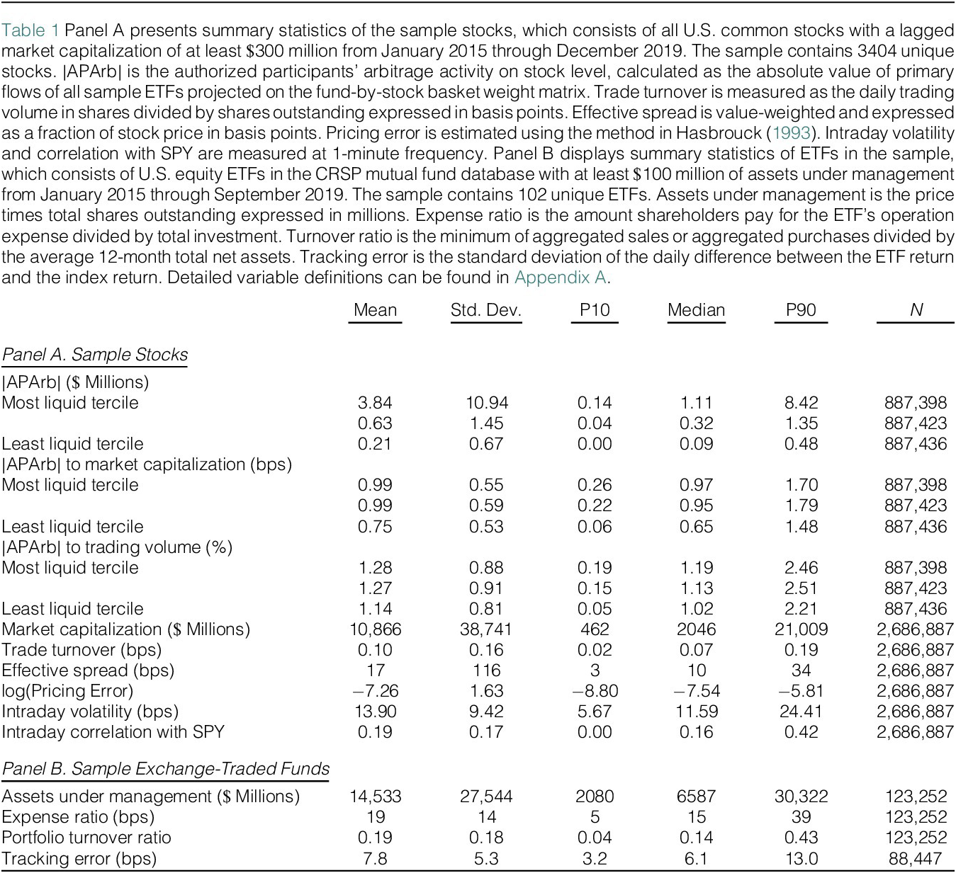
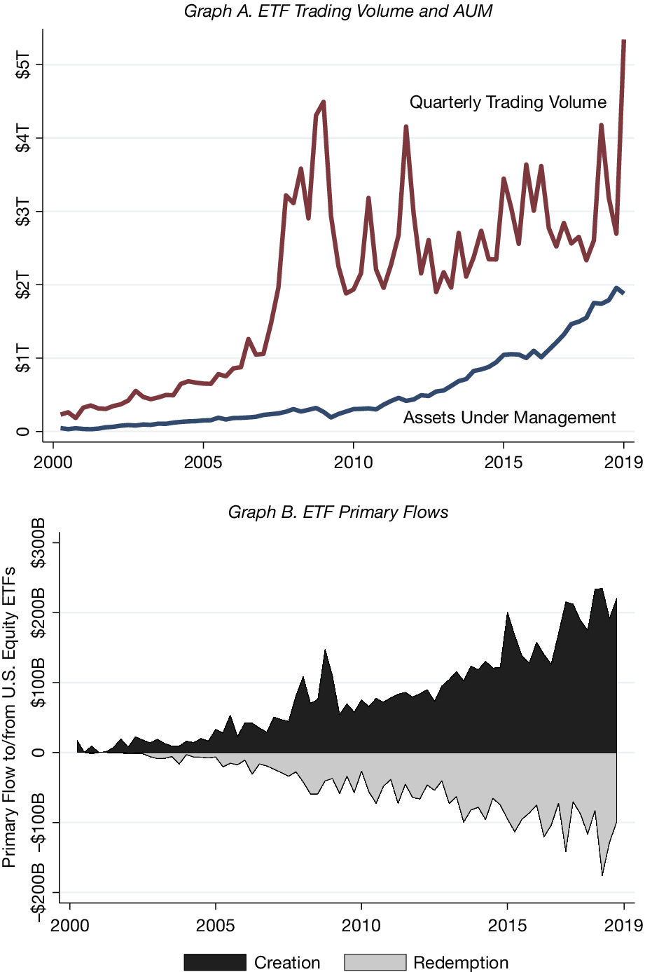
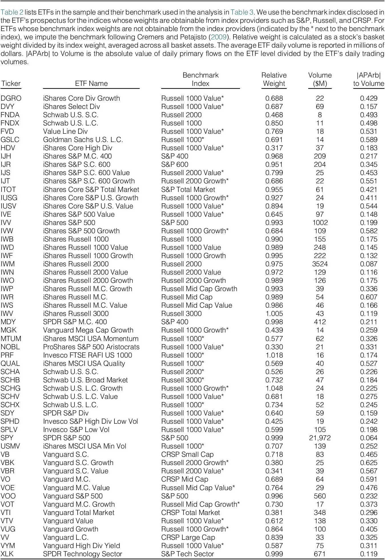
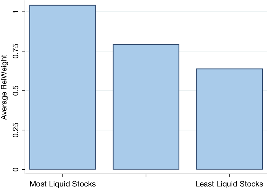
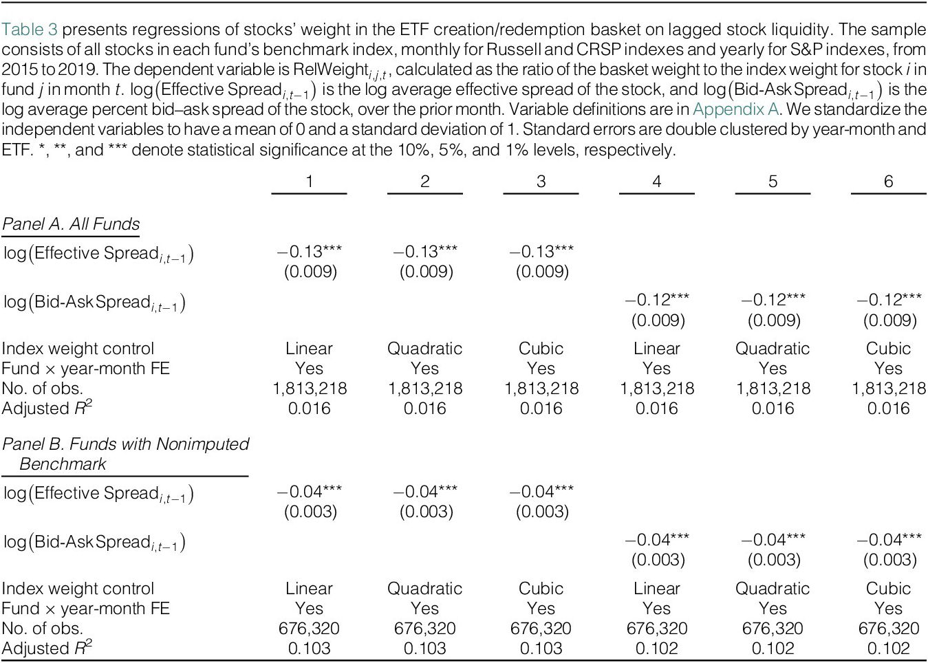
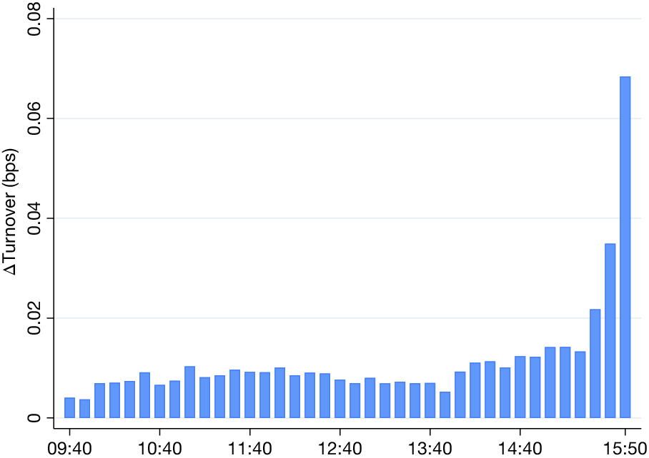
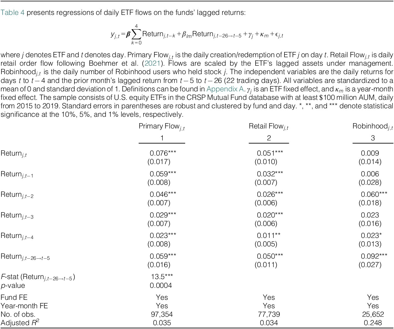
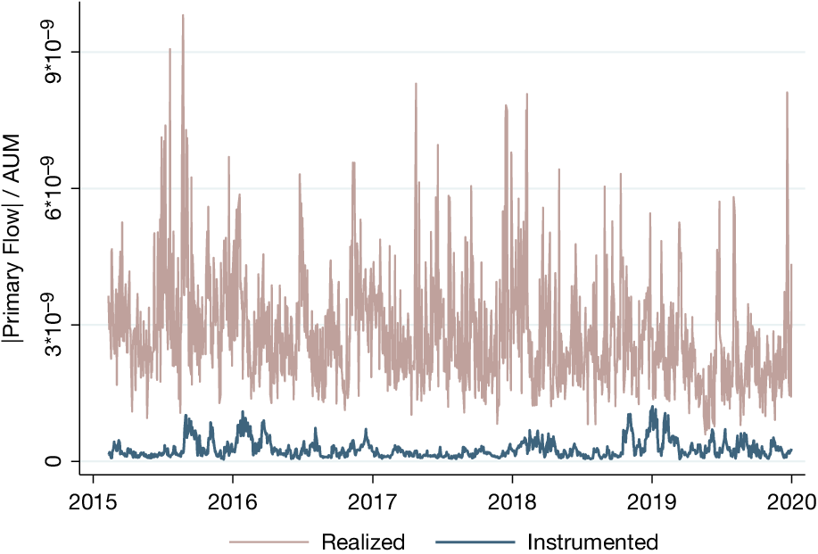


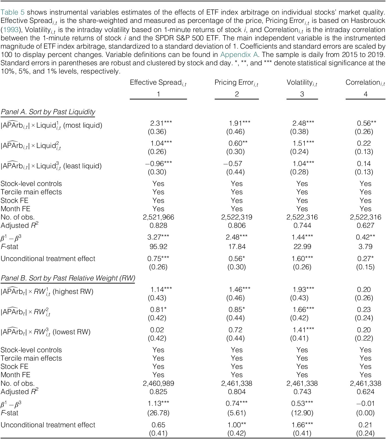
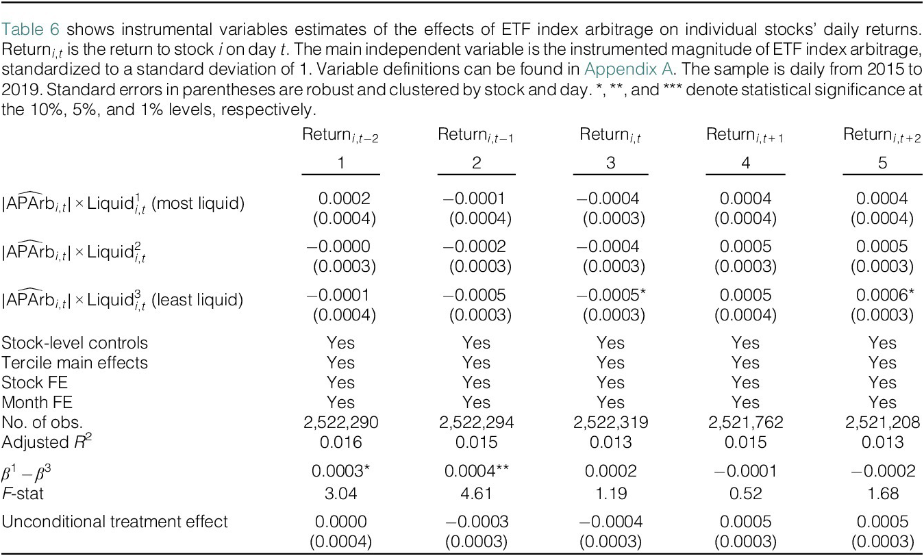
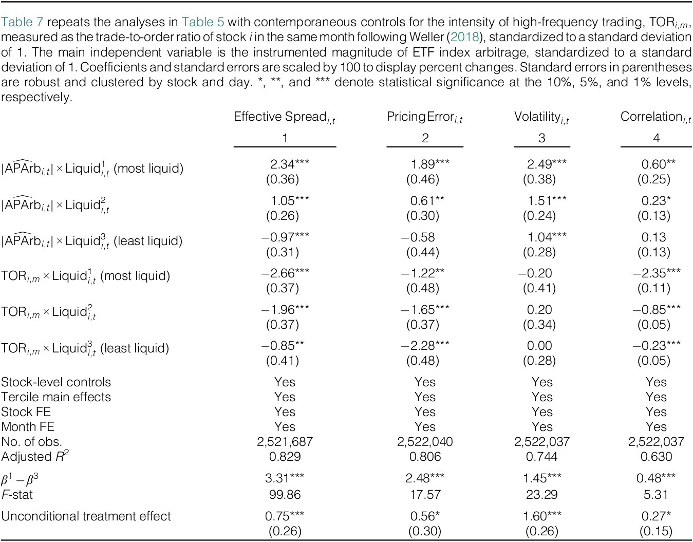
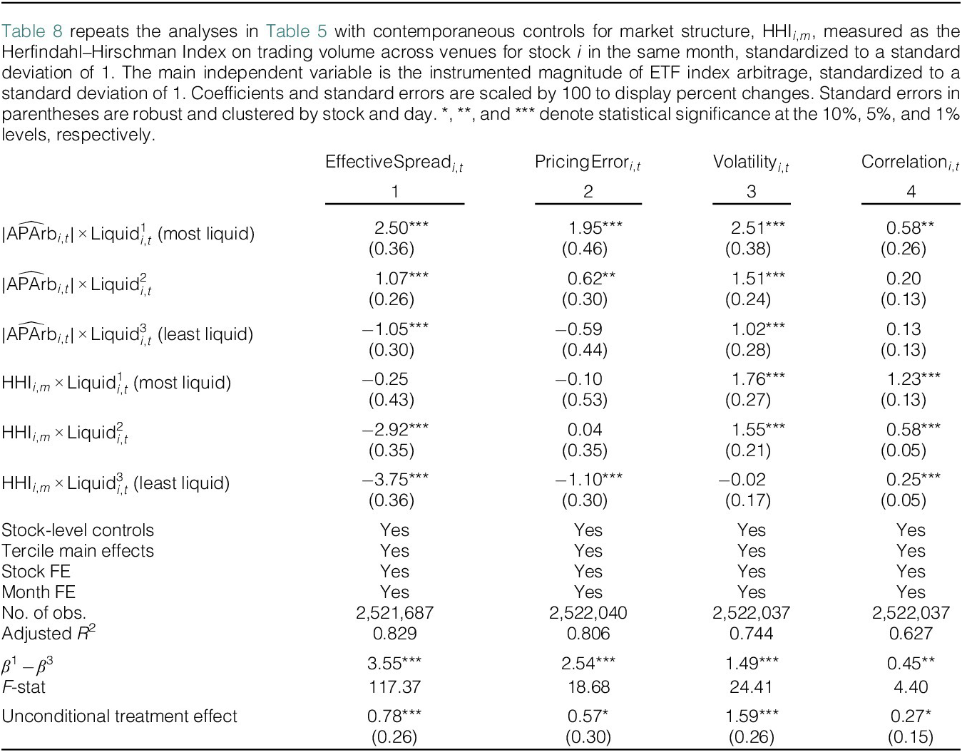
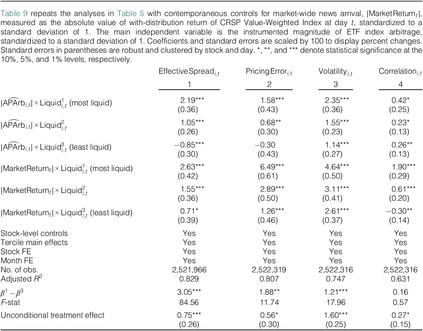


 Open access