Limitations of existing approaches

How can we learn about the effects of closeness on political behaviour? Existing studies tend to use cross‐sectional comparisons between places, or over‐time comparisons within them. Both approaches suffer from different types of selection bias, with implications for the theoretical lessons we can draw.

First, making simple cross‐sectional comparisons between safe and competitive areas risks neglecting other factors that might drive turnout or campaign contact. Competitive districts often differ to safe ones in many ways (Gallego et al., Reference Gallego, Buscha, Sturgis and Oberski2016), which might co‐determine closeness and variation in other forms of electoral and campaign behaviour. Without making strong assumptions, we cannot interpret safe districts as a counterfactual version of their competitive counterparts. In section 2.1 of the Supporting Information I make this point empirically, highlighting how different types of voters live in competitive and non‐competitive constituencies in Great Britain.

An alternative approach is to use panel data. This involves comparing the same electoral districts (or people living in them) to themselves across multiple elections, where closeness varies over time. This adjusts for any time‐invariant features of places or people living there that might confound political behaviour.

But leveraging cross‐temporal variation introduces a new, subtle, inference problem. Over‐time comparisons only work in districts that vary in closeness between elections.Footnote ⁶ But most districts do not vary that much, as I describe in more detail in the section on measuring competitiveness. More importantly, districts that do vary tend to be quite different to the country at large, in ways that fluctuate over time in accordance with changing national election dynamics. I show this in section 2.2 of the Supporting Information.

Using movers

To resolve this pair of problems I use a mover design, focusing on those who move between constituencies over time. Rather than erroneously compare constituencies directly, or focus on the unrepresentative set that change markedly between elections, I study the individuals who happen to arrive in a competitive area with those who happen to not.

The design assumes that the assignment of ‘treatment’ – the closeness of movers’ new constituencies – is independent to future political and campaign behaviour. Plainly put, people do not strategically move based on closeness, and those with greater propensity to start turning out, or be contacted by campaigns, are no more likely to arrive in competitive constituencies.

Theoretically, this seems defensible. While some work in Britain shows migration into left or right‐leaning areas is partly driven by self‐selection (Gallego et al., Reference Gallego, Buscha, Sturgis and Oberski2016), local competitiveness is less visible and less associated with demographic characteristics or partisanship of new movers. In the most recent general election, the 10 most competitive constituencies were evenly split between Labour (4), Conservative (4), Lib Dem and SNP (1 each).Footnote ⁷ And at the individual‐level, in the section on measuring competitiveness, I provide suggestive evidence that the prior demographic and political characteristics of movers do not predict the closeness of where they end up.

Data

I use data from the British Election Study Internet Panel (BESIP) (Fieldhouse et al., Reference Fieldhouse, Green, Mellon, Bailey, de Geus, Schmitt and van der Eijk2021), a large‐scale longitudinal survey of the British public. Based on respondents’ constituency, I merge this with official election results from the House of Commons Library.Footnote ⁸ Across the elections under study, constituency boundaries remain unchanged.

The BESIP has two advantages over most surveys. The first is its longitudinal structure, surveying the same respondents multiple times. The second is sample size. Each wave interviews around 30,000 people, significantly more than most GB‐wide public opinion polls. Importantly, this means that there is sufficient statistical power to detect effects, even after subsetting on those who move home.

I use two distinct samples for the analysis. The 2017 sample uses data from waves 6 and 13, fielded just after the 2015 and 2017 general elections respectively. The 2019 sample uses waves 13 and 19, taken just after the 2017 and 2019 votes. Section 1 of the Supporting Information describes the BESIP, and measures used, in further detail.

Measuring movers

I define movers as respondents whose constituency changes between survey waves. This does not directly capture whether a respondent changes house, as a respondent might move within the same local area, but rather whether they arrive in a new parliamentary jurisdiction.Footnote ⁹

Table 1 demonstrates the size of each group in the elections under study. While only a small proportion of respondents move between the 2015/2017 and 2017/2019 elections, the number that do so is high. More than 1,000 individuals change constituency between each survey wave, all of whom are observed twice – before and after they move – in the two‐period panels. This leaves more than 2000 movers in the panel datasets used for the analysis, a larger sample size than many nationally representative surveys and public opinion polls conducted in Britain.

Table 1. Movers and non‐movers proportions (BES internet panel)

Measuring competitiveness

Measuring competitiveness is conceptually challenging. While many studies simply take the constituency‐level margin of victory as a proxy, this is unsatisfying as the importance of victory margin is nonlinear; if the margin fell from 15 to 5 per cent, for example, we might expect voters to notice and parties to change strategies. If the margin fell from 60 to 50 per cent, the seat remains ‘safe’ and so turnout is less likely to change in response.

Figure 1 shows general trends in constituency competition across the British elections under study. Panel (a) shows that there is significant variation in margin of victory, but that this doesn't tend to shift too much between elections. The average constituency had a victory margin of around 23 per cent across this period. Panel (b) reaffirms this point, plotting the change in margin of victory in 2017 (vs 2015) and 2019 (vs 2017). In most constituencies, absolute victory margin changes by less than 10%.

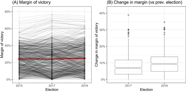
Figure 1. Trends in constituency competitiveness. Panel (a) plots the margin of victory in each constituency for the 2015–2019 general elections. The red line marks the average, which stayed constant at around 23 per cent. Panel (b) plots the change in absolute victory margin for constituencies, compared to the previous election. The distributions are very similar in 2017 and 2019, with the median rising from 7 to 9 per cent across this period.

I classify seats as ‘safe’ or ‘competitive’ by whether their victory margin falls above or below given cut‐offs. This type of approach is common in British politics, with constituencies won by less than 5 or 10 per cent often described as “swing seats” and a mark of being competitive (McInnes, Reference McInnes2020).

Using a discrete approach sidesteps non‐linearity concerns in the importance of victory margin. The biggest drawback is that results risk being sensitive to one particular cut‐off over another. I present results for all cut‐offs between 1 and 20 per cent, to evaluate if results are comparable across this range.

Figure 2 visualises the number of constituencies falling below each margin cut‐off, alongside the number that newly enter and leave, at 5 per cent intervals, across each election. As the cut‐off rises so too does the number of seats (panel a), increasing the pool of constituencies from which a mover design can draw variation. By contrast, there are fewer constituencies that newly become, or cease to be, competitive between elections (panels b‐c). This smaller, less representative group are those from which a conventional panel design would draw identifying variation.

Figure 2. Distribution of constituencies with victory margins that a) are beneath each cut‐off, b) fall below each cut‐off and so become competitive, and c) rise above each cut‐off and so become safe.

Measuring political behaviour

I analyse two facets of individual‐level behaviour: voter turnout and exposure to campaign contact. I measure turnout with retrospective participation questions, which are put to respondents in the survey wave immediately following an election to minimise false recall (Dassonneville & Hooghe, Reference Dassonneville and Hooghe2017). All questions include text saying that many people were unable to vote, to reduce social desirability bias (see Krumpal, Reference Krumpal2013).

Nonetheless, self‐reported turnout in the panel remains high. In the immediate post‐election waves between 2015–2019, 93, 91.9 and 91 per cent of respondents report having voted. By contrast, the true turnout rate in each election (excluding Northern Ireland) was 66.4, 68.9 and 67.5 per cent, respectively. Unlike the full British Election Study, the internet panel does not provide validated turnout data, so it is not possible to measure false reporting nor adjust for it in the analysis.

Overreporting of turnout is common to national election studies (Jackman & Spahn, Reference Jackman and Spahn2019), and might place ‘ceiling effects’ on the analysis that make it harder to detect changes. I discuss this possibility in more detail later, particularly given the general null findings in turnout specifications.

In other ways, though, it need not pose a direct threat to causal inference. Overreporting is likely due to continued social desirability, and the fact that BESIP panellists might be more politically engaged than the wider population. Among movers, neither are likely related to the competitiveness of one's new constituency. And second, any underlying personality traits that drive false reporting are reasonably addressed by using individual fixed effects.

Measuring campaign contact is more straightforward, with a binary question that asks if any of the main political parties contacted respondents. This general measure encapsulates various ways parties communicate with voters, like door‐knocking, leafleting, or online advertising. I explore more specific outcomes in section 5.1 of the Supporting Information, alongside the empirical results presented in the main text.

Across the three post‐election waves there is more variation in responses, with between 47.7 and 59.8 per cent reporting contact. These results vary for each specific mode of contact, as outlined in the Supporting Information.

Estimation

I estimate close election effects across a series of individual‐level, two‐way fixed effects specifications. For individuals $i$$i$ in constituency $c$$$c and election year $t$$t$, I regress individual‐level turnout or campaign contact $y_{ict}$${{y}_{ict}}$ on constituency type ${\theta }_{ict}$${{\theta }_{ict}}$, accounting for individual and election‐year fixed effects ${\gamma }_i$${{\gamma }_i}$ and ${\alpha }_t$${{\alpha }_t}$ respectively. Standard errors are clustered at the individual‐level throughout.

I use distinct two‐period panels for the analysis, studying 2015–17 and 2017–19 movers separately. This makes estimation comparable to a canonical 2 × 2 difference‐in‐differences design, sidestepping recent econometric concerns about the validity of two‐way fixed effects (Callaway & Sant'Anna, Reference Callaway and Sant'Anna2021).

${\theta }_{ict}$${{\theta }_{ict}}$ is a three‐level factor, with the baseline that a mover's constituency type does not change. This allows us to disentangle effects among movers who relocate from safe to close seats, and from close to safe seats, maintaining a common counterfactual that absorbs any direct effects of moving.

These specifications estimate an average treatment effect on the treated (ATT) in which the treated group is those who move to a different type of constituency. In what follows I refer to this as the “mover ATT”.

$y_{ict}={\beta }_1{\theta }_{ict}+{\gamma }_i+{\alpha }_t+{\epsilon }_{ict}$$$\begin{equation*}{{y}_{ict}} = {{{{\beta}}}_1}{{{{\theta}}}_{ict}} + {{{{\gamma}}}_i} + {{{{\alpha}}}_t} + {{\epsilon }_{ict}}\end{equation*}$$

Identification

For ${\beta }_1$${{\beta }_1}$ to yield causal interpretation, we must assume that the competitiveness of movers’ destination constituency is independent to potential outcomes (participation or campaign exposure). To test this, I model the type of constituency to which respondents will move as a function of their demographic and political characteristics.Footnote ¹⁰ I do this for all cut‐offs between 1 and 20 per cent, and plot the resulting 20 p‐values for each variable in each election in Figure 3 (full results section 3.1 of the Supporting Information). As evidenced by the lack of red and blue dots, which indicate p values below 5 and 10 per cent, respectively, no characteristics consistently breach conventional levels of statistical significance. While independence cannot be empirically proven, these results provide strong suggestive support.

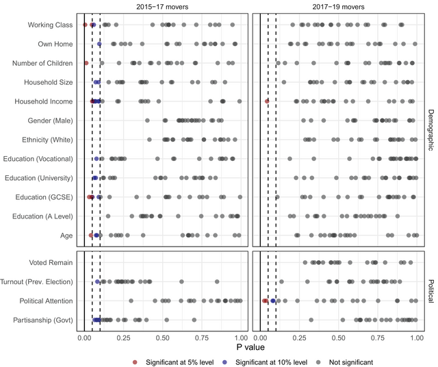
Figure 3. Modelling covariate balance across future mover destinations. The figure plots the p‐values from a regression that models movers’ change in constituency type, i.e. their treatment assignment, as a function of their demographic and political characteristics. Dashed lines represent 5 and 10 per cent significance levels. Remain vote variable not included for the 2015 sample, as the vote did not take place until 2016. Full results in section 3.1 of the Supporting Information.

Main effects

The results of the main specifications are presented below. Since the dependent variable is a binary indicator of turnout or campaign contact, the coefficients can be interpreted probabilistically; each mover ATT represents the change in probability that a respondent reports having voted, or being contacted, in the first general election after they move to a given type of constituency. Results are presented across a series of cut‐offs for what counts as a competitive seat, ranging from a victory margin of 1 through to 20 per cent.

Minimal effects on turnout

To begin, Figure 4 presents mixed effects on individual‐level voter turnout. Looking first at the 2017 election (upper panels), against expectations both sets of models yield negative coefficients. While this makes sense for those moving to safe seats, it is puzzling for those moving to more competitive parts of the country, for whom effects are if anything more robust. Nonetheless, many of the estimates fail to reach conventional levels of statistical significance, and vary substantively across cut‐offs.

Figure 4. Mover ATT estimates for self‐reported turnout. Full results in section 4.1 of the Supporting Information.

In 2019 (lower panels) the evidence is similarly mixed. While moving to a safe seat reduces turnout at some of the highest percentage cut‐offs, effects elsewhere are inconsistent and usually fail to reach statistical significance, so do not yield firm substantive conclusions.

Overall, these results do not provide strong indication that moving to a safe or competitive constituency affects voter turnout. Part of this lack of effect may stem from over‐reporting, or above‐average true political participation among panellists, placing a ceiling on the findings. It might also highlight selection effects in existing cross‐sectional and panel research designs, which sometimes report significant results.

Stronger effects on campaign contact

There is stronger evidence that moving to a new type of constituency impacts the likelihood of being contacted by political parties. Figure 5 presents effects on general self‐reported contact in the election campaign. Particularly in 2017 (upper left), moving to a safe seat has more consistent negative effects on contact, which are statistically significant at a wide range of cut‐offs. Positive effects from competitive constituencies are routinely positive and significant in 2019 (lower right), and point in a similar direction two years before.

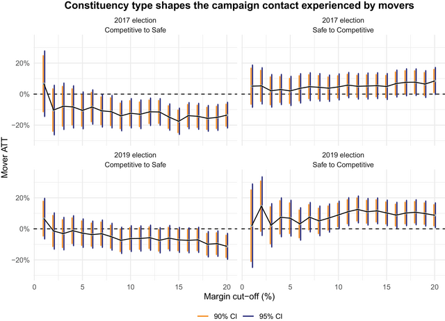
Figure 5. Mover ATT estimates for general campaign contact. Full results in section 4.2 of the Supporting Information.

One problem with these results, though, is that they rely on a general outcome measure which collates many different types of campaign contact. If competition is driving exposure to campaigns among movers, we might expect these effects to be driven by more costly modes of campaigning, which parties must strategically allocate across seats. One such form of campaign contact is whether or not respondents are ‘visited’ by party activists. Visits, sometimes referred to as ‘canvassing’, are a core part of parties’ mobilisation efforts in British elections (see: Johnston et al., Reference Johnston, Cutts, Pattie and Fisher2012).

Figure 6 presents results using this outcome, and the effects become more marked. Moving to a safe seat sees reported canvassing decline in both elections, while moving to a competitive seat sees it increase in 2019. These effects are particularly robust for safe‐seat movers in 2017 (upper left), where 85 per cent of coefficients are significant at the 10 per cent level, and competitive‐seat movers in 2019 (bottom right), where 95 per cent are as such. In section 5.1 of the Supporting Information I examine effects for other modes of campaign contact.

Figure 6. Mover ATT estimates for party canvassing. Results for other modes of contact in section 5.1 of the Supporting Information.

Taken together, these findings suggest that exposure to campaign contact is likely shaped, at least in part, by the type of constituency to which one moves. These effects appear driven by in‐person forms of campaigning, to which parties strategically allocate resources based on perceptions of how likely they are to win the vote.

External validity

The results throughout this research note present effects among movers. But how might these generalise to the wider population, and be of wider theoretical consequence?

One way to gauge the external validity of the estimates is to see how representative movers are of the wider BES sample. I compare the political and demographic characteristics of future movers and non‐movers, to understand how movers might differ.

Figure 7 presents the results, from which two key trends emerge. First, movers are not a demographic mirror of the full sample: they tend to be younger, less working class, less likely to own a home, less likely to have children, and more likely to be university educated.

Figure 7. Cross‐sectional differences in the probability of moving house between elections. Coefficients represent the change in probability of moving, compared to not moving. Remain vote variable not included for the 2015 sample, as the vote did not take place until 2016. Full results in section 3.2 of the Supporting Information.

Many of these findings are intuitive, given the logistics of moving. For instance, moving is more difficult for those who own a home or have children, while younger, university educated, middle class people tend to be more geographically mobile in the labour market.

How these differences relate to voter turnout, though, is less clear. On the one hand, existing work suggests that better educated, more middle class voters are more likely to participate in elections (Evans & Tilley, Reference Evans and Tilley2017; Smets & van Ham, Reference Smets and van Ham2013). So too are voters without children (Bellettini et al., Reference Bellettini, Ceroni, Cantoni, Monfardini and Schafer2023; Bhatti et al., Reference Bhatti, Hansen, Naurin, Stolle and Wass2019), so, a priori, movers should have more proclivity to participate. On the other hand, the fact that movers are younger and less likely to own property might have effects in the opposite direction. There is significant evidence that young people are less likely to vote in elections (Smets & van Ham, Reference Smets and van Ham2013), particularly in Britain (Prosser et al., Reference Prosser, Fieldhouse, Green, Mellon and Evans2020), while property ownership, as means to holding a permanent stake in local politics, has long been viewed as a determinant of participation (Brady et al., Reference Brady, Verba and Schlozman1995). Taking all these factors together, it is not clear whether movers are the types of people we should necessarily expect to vote more, or less, than the wider public.

Despite demographic differences, however, movers are generally more politically comparable with the broader sample. They are no more or less likely to have voted in the last election before moving, have similar levels of self‐reported political attention, and chose similarly in the EU referendum. The only difference is that 2017 movers are slightly more likely to identify as government supporters (in 2015), but this effect is substantively small (around 1.5 per cent), and significantly smaller than the comparable effects of age and home ownership.

A reasonable conclusion to draw, then, is that while movers are not a perfect snapshot of the general public, they provide a consistent and reasonably politically representative sample. This gives scope for cautious generalisation, potentially more so than in some existing cross‐sectional and panel designs.