


1. Introduction
Radio-echo sounding (RES) is commonly used to survey glaciers and ice sheets (e.g., Schroeder and others, Reference Schroeder2020), with the predominant target being the ice-bed interface to provide an estimate of the total ice-sheet volume (e.g., Pritchard and others, Reference Pritchard2025). Additional information is preserved within the ice column, where contrasts in conductivity or permittivity, typically associated with changes in the ice impurity content (Gudmandsen, Reference Gudmandsen1975; Eisen and others, Reference Eisen, Wilhelms, Nixdorf and Miller2003) or crystal orientation fabric (Fujita and others, Reference Fujita1999; Gerber and others, Reference Gerber, Lilien, Nymand, Steinhage, Eisen and Dahl-Jensen2025), create englacial reflections. Some of these englacial layers are horizontal and smooth relative to the transmitted radar wavelength because they were deposited uniformly as continuous horizons and buried over time, and together the continuous englacial layers form a stratified set of coherent reflections comprising the ‘radiostratigraphy’ (MacGregor and others, Reference MacGregor2015). Smooth layers create specular radar reflections, where most energy is reflected at the incident angle. In the case of a highly specular horizontal layer and a nadir-looking radar, all the reflected energy is directed back to the receiver. For this reason, the relatively flat near-surface layers in the accumulation area of an ice sheet are extraordinarily well resolved and can be connected over 100s of km between ice cores (e.g., Cavitte and others, Reference Cavitte2021; Bingham and others, Reference Bingham2025).
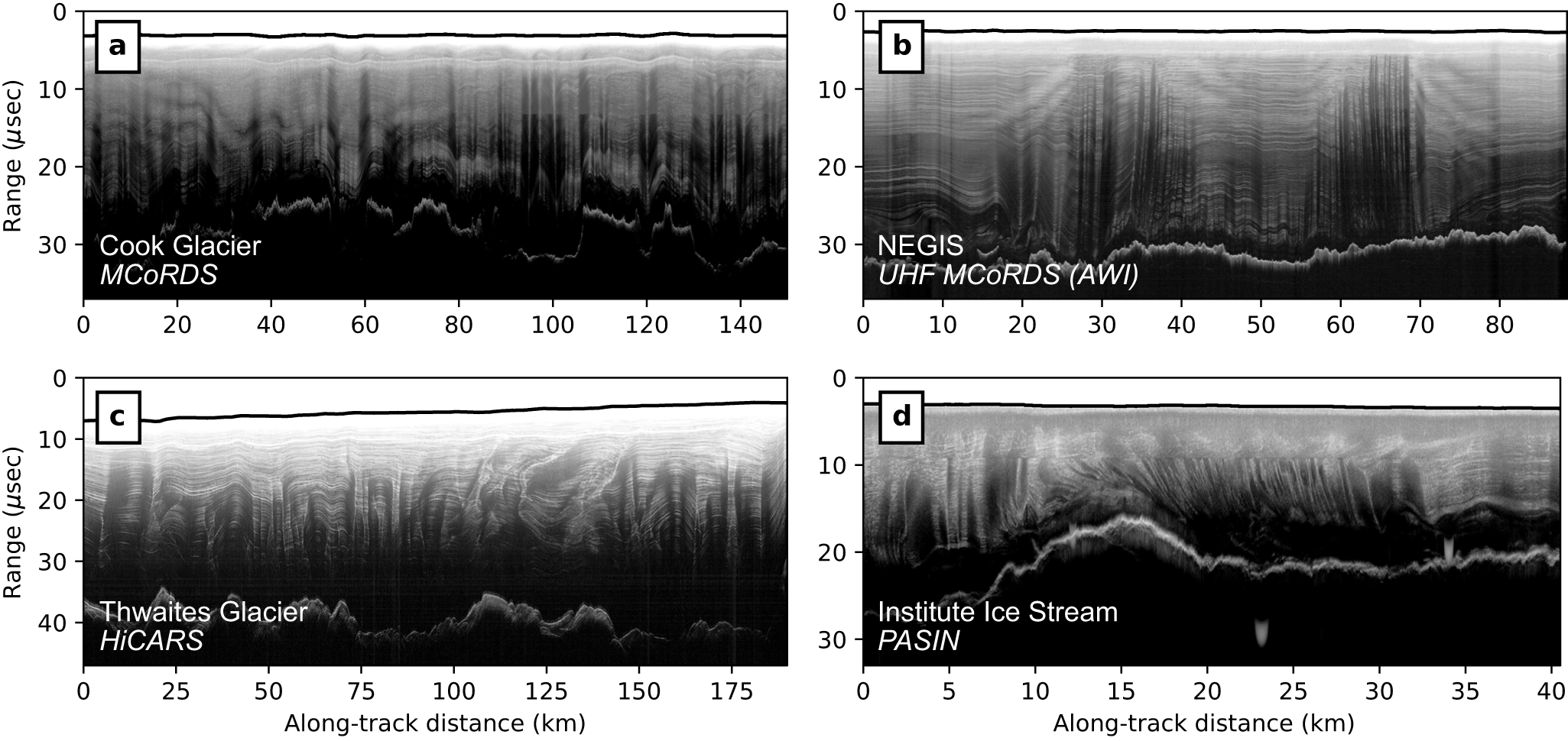
In other glacier settings, layers are not flat; for example, near the glacier bed, layers can conform to the bed topography, even in high-relief regions (e.g., Hudleston, Reference Hudleston2015). In highly dynamic areas, layers may not be flat nor conform to the bed. Layers can be distorted by ice flow (e.g., Jacobel and others, Reference Jacobel, Gades, Gottschling, Hodge and Wright1993; Holschuh and others, Reference Holschuh, Parizek, Alley and Anandakrishnan2017) or mass exchange at the bed (e.g., Bell and others, Reference Bell2011; Jordan and others, Reference Jordan2018), and they can therefore preserve a history of paleo ice dynamics (e.g., Conway and others, Reference Conway, Catania, Raymond, Gades, Scambos and Engelhardt2002; Siegert and others, Reference Siegert, Ross, Corr, Kingslake and Hindmarsh2013). In any case, layer dips can be much steeper compared to the flat ice-sheet surface. Then, a dipping specular layer may be resolvable only by an off-nadir propagating wave, orthogonal to the layer dip. For this reason, received radar power is often diminished for dipping layers (Holschuh and others, Reference Holschuh, Christianson and Anandakrishnan2014), sometimes generating anomalous vertical features within the RES image which have been called ‘tornadoes’ or ‘whirlwinds’ (Karlsson and others, Reference Karlsson, Rippin, Vaughan and Corr2009; Winter and others, Reference Winter2015) (Fig. 1).

Figure 1. Examples of poorly resolved dipping layers in radar-sounding images: (a) Cook Glacier imaged with the Multi-channel Coherent Radar Depth Sounder (MCoRDS) (Open Polar Radar, 2024); (b) The Northeast Greenland Ice Stream (NEGIS) imaged with an ultra-high frequency version of MCoRDS (Franke and others, Reference Franke2022); (c) Thwaites Glacier imaged with the High-Capability Airborne Radar Sounder (HiCARS) (Schroeder and others, Reference Schroeder, Blankenship and Young2013); (d) Institute Ice Stream imaged with the Polarimetric Airborne Science INstrument (PASIN) (Winter and others, Reference Winter2015). Vertical or near-vertical dark streaks that interrupt englacial stratigraphy are locations where signals from nadir and off-nadir destructively interfere in standard RES processing frameworks. Profiles are plotted as a measured range in time from the radar instrument, with the ice surface shown as a solid black line.
RES antennas have a small real aperture, meaning that the real beam width is large and some portion of the radar wave is directed off nadir (Heister and Scheiber, Reference Heister and Scheiber2018). It is therefore expected that radar power should be received from dipping specular layers, but that those signals may not be apparent depending on whether they are summed coherently during focusing. In the cross-track direction, multiple antenna elements can be used together in an array to steer the radar beam toward off-nadir targets (Paden and others, Reference Paden, Akins, Dunson, Allen and Gogineni2010), enabling swath mapping of the glacier bed (Holschuh and others, Reference Holschuh, Christianson, Paden, Alley and Anandakrishnan2020) among other applications. In the along-track direction, signals are coherently averaged within a synthetic aperture as the antenna moves between acquisitions (Legarsky and others, Reference Legarsky, Gogineni and Akins2001; Peters and others, Reference Peters, Blankenship and Morse2005), as is done in spaceborne synthetic aperture radar (SAR) applications (Cumming and Wong, Reference Cumming and FHc2005). The SAR algorithms used in RES are generally optimized for targets that are rough at the scale of the radar wavelength (we use the term ‘diffuse’ here), which scatter energy in all directions and are therefore observable from many angles across the synthetic aperture. Then, one can coherently average through a set of look directions around that of the real beam, constructively interfering signals to raise the signal power and narrow the along-track resolution. However, for targets that are both specular and off-nadir, the nadir-looking reference function (used in SAR processing) may not match the shape of the signal return. Incorrectly applying that reference function would diminish, rather than amplify as intended, the output signal, which we are here calling destructive interference (not to be confused with destructive presumming) (Holschuh and others, Reference Holschuh, Christianson and Anandakrishnan2014).
Here, we give context on the SAR algorithms commonly used for glaciological sounding in terms of their ability to resolve dipping englacial layers. Then, we describe two alternative methods that are better suited for considering all types of englacial reflectors together (including dipping specular layers), or a rough ice surface, both using synthetic squint angles to steer the radar beam toward orthogonal incidence with dipping layers. The first method was previously described by Heister and Scheiber (Reference Heister and Scheiber2018), but has not been commonly used for resolving radiostratigraphy, and the second method we developed here and has never before been implemented to our knowledge. We apply these methods in along- and across-flow radar profiles at Academy Glacier, East Antarctica. The improved result can be used for better interpretations of individual layers of interest and to generate more precise glaciological (e.g., Catania and others, Reference Catania, Scambos, Conway and Raymond2006; Sanderson and others, Reference Sanderson2023) and paleoclimatological (e.g., Bodart and others, Reference Bodart, Bingham, Ashmore, Karlsson, Hein and Vaughan2021; Lilien and others, Reference Lilien2021) insight.
2. Background
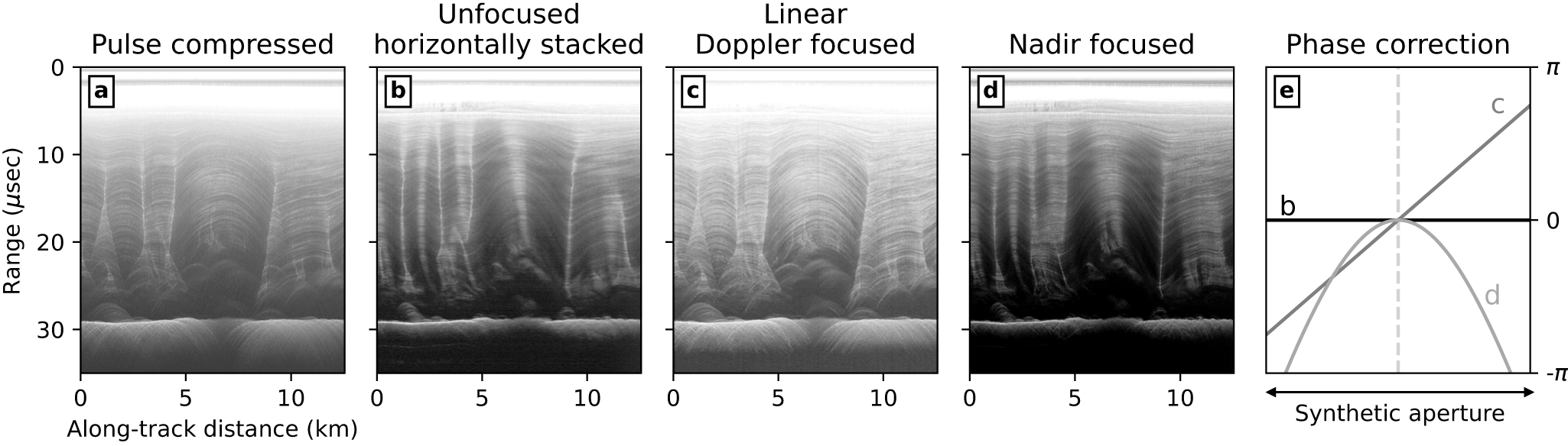
To generate images for interpretation, ‘fast-time’ (range) and ‘slow-time’ (along-track or ‘azimuth’) filtering are performed on radar-sounding data. Fast-time matched filtering (often called pulse compression) localizes energy from a finite-duration pulse to the range bins associated with the scattering target. This type of compression is not the focus of this work, and we use pulse-compressed data as a starting point for our analyses (Fig. 2a). Here, we consider different strategies for along-track compression, which can be thought of both as strategies to focus images and improve their signal-to-noise ratio (SNR). The simplest and least computationally expensive method for along-track compression is with no range correction to signal phase before horizontally summing neighboring traces (called presumming or stacking); this processing strategy can raise the SNR and lower the data volume (generating unfocused imagery, or ‘quicklook’ in Open Polar Radar (OPR) 2024; Fig. 2b). To coherently focus the image (i.e., sum received radar signals after having aligned their phase), one must estimate how the range to target is expected to change through the synthetic aperture and apply the along-track compression with that range/phase adjustment. In this section, we describe two commonly implemented focusing methods and how they can be used to resolve dipping englacial layers.

Figure 2. A single radar image processed with four common SAR techniques: (a) pulse compressed; (b) unfocused horizontally stacked (‘quicklook’); (c) linear Doppler focused (‘LOSAR’); (d) nadir-focused with  $f$-
$f$- $k$ migration (‘standard’). (e) Hypothetical phase corrections within a synthetic aperture for each method (b–d). Data are from and processing is done through Open Polar Radar (2024).
2.1. Linear Doppler focusing
The radar-sounding instruments designed for generating radar profiles are on moving platforms, so the range to a target and the associated phase offset between neighboring returns change through the synthetic aperture. The phase,  $\phi$, gradient in along-track time, $\eta$ (slow time), is the so-called Doppler frequency, $f_\mathrm{D}$, given as
 \begin{equation}
2\pi f_\mathrm{D} = \frac{\partial \phi}{\partial \eta}\;.
\end{equation}
\begin{equation}
2\pi f_\mathrm{D} = \frac{\partial \phi}{\partial \eta}\;.
\end{equation} Measured returns can come across the full Doppler spectrum, even for a single target if it is diffuse, but they are only resolvable within the Doppler bandwidth,  $B_\mathrm{D}$
 \begin{equation}
B_\mathrm{D} = \frac{v}{\Delta x}
\end{equation}
\begin{equation}
B_\mathrm{D} = \frac{v}{\Delta x}
\end{equation} set by the platform velocity,  $v$, and acquisition spacing, $\Delta x$.
Specular targets may only be expressed across some subset of the full Doppler spectrum, centered on the Doppler centroid (the Doppler frequency with greatest power,  $f_{\mathrm{Dc}}$), which is (Heister and Scheiber, Reference Heister and Scheiber2018; Castelletti and others, Reference Castelletti, Schroeder, Mantelli and Hilger2019)
 \begin{equation}
f_{\mathrm{Dc}} = \frac{2 v f_\mathrm{c}}{c}\sqrt{\epsilon_\mathrm{r}}\sin\theta
\end{equation}
\begin{equation}
f_{\mathrm{Dc}} = \frac{2 v f_\mathrm{c}}{c}\sqrt{\epsilon_\mathrm{r}}\sin\theta
\end{equation} where  $f_\mathrm{c}$ is the instrument center frequency, $c$ is the vacuum wave speed, $\epsilon_\mathrm{r}$ is the relative permittivity of the near-field material ( $\epsilon_\mathrm{r}=1$ for airborne platforms) and $\theta$ the near-field ray propagation angle ( $\theta=0$ being directly downward, nadir). Then, for normal incidence with an englacial target, it must be dipping at some angle, $\theta_\mathrm{ice}$, which can be found by rearranging equation 3 and applying Snell’s law on refraction from the near-field into the ice,
 \begin{equation}
\sin(\theta_\mathrm{ice}) = \frac{c f_{\mathrm{Dc}}}{2 v f_\mathrm{c} \sqrt{\epsilon_\mathrm{ice}}}
\end{equation}
\begin{equation}
\sin(\theta_\mathrm{ice}) = \frac{c f_{\mathrm{Dc}}}{2 v f_\mathrm{c} \sqrt{\epsilon_\mathrm{ice}}}
\end{equation} where  $\epsilon_\mathrm{ice}$ is the relative permittivity of ice ( $\sim$3.15). Inspecting the Doppler centroids directly can therefore give broad insight into englacial features (Arenas-Pingarrón and others, Reference Arenas-Pingarrón2025), which we discuss further in Section 5.
Doppler centroids can also be used for a type of SAR focusing that assumes a linear phase correction through the synthetic aperture (i.e., constant frequency)
 \begin{equation}
\Delta \phi = 2\pi f_\mathrm{Dc} \frac{\Delta x}{v}
\end{equation}
\begin{equation}
\Delta \phi = 2\pi f_\mathrm{Dc} \frac{\Delta x}{v}
\end{equation}and can be applied adaptively for each pixel in the image (Fig. 2c). Castelletti and others (Reference Castelletti, Schroeder, Mantelli and Hilger2019) implemented this layer-optimized SAR (LOSAR) technique in the time domain. LOSAR images have better-resolved radiostratigraphy compared to prior data products. However, the LOSAR algorithm assumes perfect specularity; that is, it only considers power at a single Doppler frequency (the centroid). It also assumes that targets are linear within the synthetic aperture, which can lead to unrealistic abrupt changes in angles in the processed image if the Doppler centroids are noisy, especially since this method does not include any range migration. Alternatively, if the expected shape of the target is known, can be exhaustively searched for, or can be determined from measured Doppler spectra, an arbitrary reference function could be used to coherently focus over a much larger aperture (Schroeder and others, Reference Schroeder, Castelletti and Pena2019).
2.2. Conventional nadir focusing
Conventional focusing methods accommodate a range of frequencies across the Doppler spectrum, making diffuse and specular targets differentiable (Fig. 2d). Considering a nadir-looking synthetic aperture, the target comes into view approaching the instrument (positive Doppler frequency), eventually reaches some point of closest approach (zero Doppler), then goes out of view behind (negative Doppler). The frequencies are defined through a function for the expected equivalent range,  $r$, with possible ray bending from the near-field into the ice surface,
 \begin{equation}
r = r_\mathrm{near} + r_\mathrm{ice} = \sqrt{\epsilon_\mathrm{near}}\sqrt{h^2 + (x-s)^2} + \sqrt{\epsilon_\mathrm{ice}}\sqrt{d^2 + s^2}
\end{equation}
\begin{equation}
r = r_\mathrm{near} + r_\mathrm{ice} = \sqrt{\epsilon_\mathrm{near}}\sqrt{h^2 + (x-s)^2} + \sqrt{\epsilon_\mathrm{ice}}\sqrt{d^2 + s^2}
\end{equation} where  $h$ is the length scale for the near-field permittivity (for airborne platforms, the height of the aircraft above the ice surface), $d$ is the depth of the target below the ice surface, $x$ is the along-track distance and $s$ is the along-track position for refraction from near-field to ice (the air-ice interface) (Hélière and others, Reference Hélière, Lin, Corr and Vaughan2007). We refer to $r$ in equation (6) as an ‘equivalent’ range because it is not a true distance but is convenient for its simple relation to phase by $\phi = 4 \pi r f_\mathrm{c}/{c}$ and then to frequency through equation (1). Thus, a given target has an approximately linear frequency ramp (or hyperbolic phase) through the synthetic aperture (Fig. 2e).
The maximum resolvable Doppler frequency (and hence maximum layer dip through equation (4)) is set by the Doppler bandwidth, equation (2). For steeply dipping reflectors, outside the Doppler bandwidth, the range-matched filter (defined by equation (6)) will lead to destructive interference and decrease the coherent signal power (Holschuh and others, Reference Holschuh, Christianson and Anandakrishnan2014). However, the maximum dip angle from which individual radar reflections can be received is instead set by the width of the radar beam and focusing effects of refraction at the ice surface,  $\theta_\mathrm{ice} = 34^\circ$ (Dowdeswell and Evans, Reference Dowdeswell and Evans2004). Since the transmitted waves are relatively low frequency ( $\sim$10–1000 MHz) and the antenna array is small in the along-track direction, the radar beam is large (Heister and Scheiber, Reference Heister and Scheiber2018), and some energy should be expected from off-nadir targets. If the raw image is downsampled during processing, as is common due to the computational inefficiency with high data volumes, a larger $\Delta x$ narrows
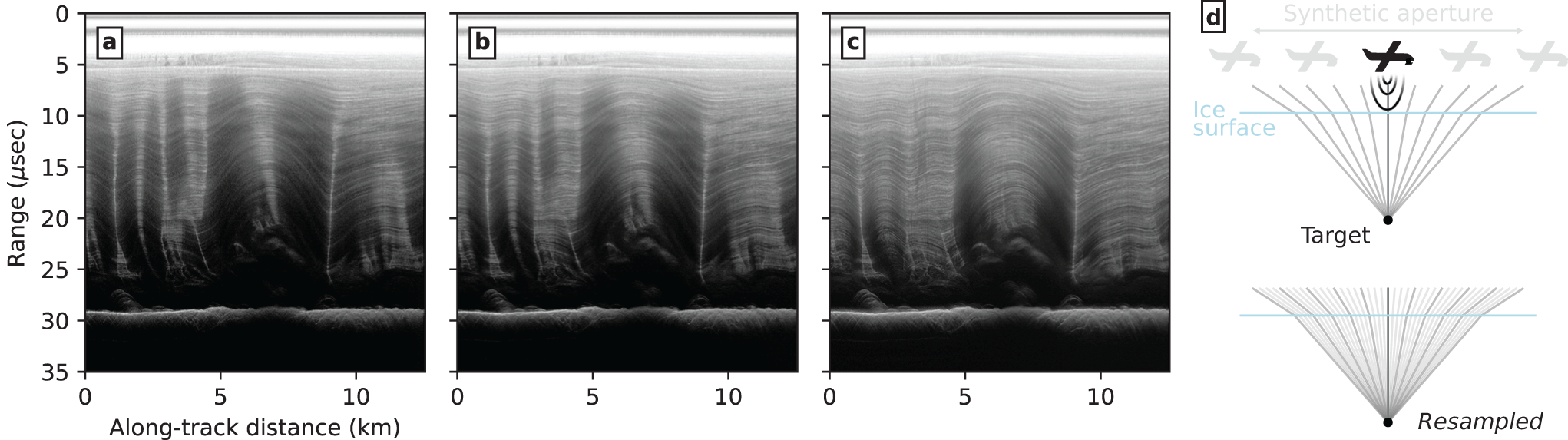
  $B_D$ to where it cannot resolve the steep layers even if those layers are reflecting individual radar returns. To extend the Doppler bandwidth with the goal to resolve more steeply dipping layers, the image can be sampled at higher resolution in the along-track dimension (Fig. 3).

Figure 3. A demonstration of how different sampling intervals in the along-track dimension—(a) 2.5 m spacing, (b) 1.5 m spacing and (c) 1 m spacing—can change the focused result. Finer along-track sampling leads to better SAR coherence for the high Doppler frequency content (i.e., dipping layers). The radar data are from the same segment as in Fig. 2. (d) An illustration of resampling the synthetic aperture.
3. Squinted SAR focusing
Resampling in the along-track dimension can expand the Doppler bandwidth, but in some cases, it may not effectively eliminate destructive interference for dipping layers. For instance, the commonly used frequency-wavenumber ( $f$-
$f$- $k$) migration (Legarsky and others, Reference Legarsky, Gogineni and Akins2001) assumes a uniformly horizontal layered geometry. A rough ice surface or short-scale variations in the ice density (and therefore radar-wave velocity) may lead to enough phase variation between acquisitions to prevent constructive interference within the synthetic aperture. Although other migration routines are capable of more complicated geometries and have been implemented for glaciological radar sounding (e.g., time-domain back propagation;
Xu and others, Reference Xu, Lang, Cui, Li, Liu, Guo and Sun2022), these are substantially more computationally expensive. Instead, we i) divide the full aperture into multiple subapertures and optionally ii) adaptively restrict a single subaperture around the signal, in either case reducing the length scale over which the geometric assumptions are made (Rodríguez and others, Reference Rodríguez, Bertran, Veeramacheneni and Belz2009), which both resolves dipping layers and allows for spatial variations in the ice surface height and ice density within the firn column.
$k$) migration (Legarsky and others, Reference Legarsky, Gogineni and Akins2001) assumes a uniformly horizontal layered geometry. A rough ice surface or short-scale variations in the ice density (and therefore radar-wave velocity) may lead to enough phase variation between acquisitions to prevent constructive interference within the synthetic aperture. Although other migration routines are capable of more complicated geometries and have been implemented for glaciological radar sounding (e.g., time-domain back propagation;
Xu and others, Reference Xu, Lang, Cui, Li, Liu, Guo and Sun2022), these are substantially more computationally expensive. Instead, we i) divide the full aperture into multiple subapertures and optionally ii) adaptively restrict a single subaperture around the signal, in either case reducing the length scale over which the geometric assumptions are made (Rodríguez and others, Reference Rodríguez, Bertran, Veeramacheneni and Belz2009), which both resolves dipping layers and allows for spatial variations in the ice surface height and ice density within the firn column.
3.1. Squinted subapertures
Consider multiple subapertures, each assigned a ‘squint’ angle to steer the radar beam in the along-track direction and toward orthogonal incidence with dipping englacial layers (Fig. 4) (Rodríguez and others, Reference Rodríguez, Bertran, Veeramacheneni and Belz2009; Ferro, Reference Ferro2019). The radar instrument may be physically or electrically squinted forward or backward to illuminate targets in front of or behind the instrument, respectively. Here, the radar antennas have zero physical squint (pointed at nadir), but since the real beam is large, we can use synthetic squint angles to distinguish subapertures within the beam. Since, in this case, the migration routine ( $f$-
$f$- $k$) is in Doppler space, the subapertures represent portions of the Doppler spectrum, with the forward squinted subaperture illuminating the highest Doppler frequencies.

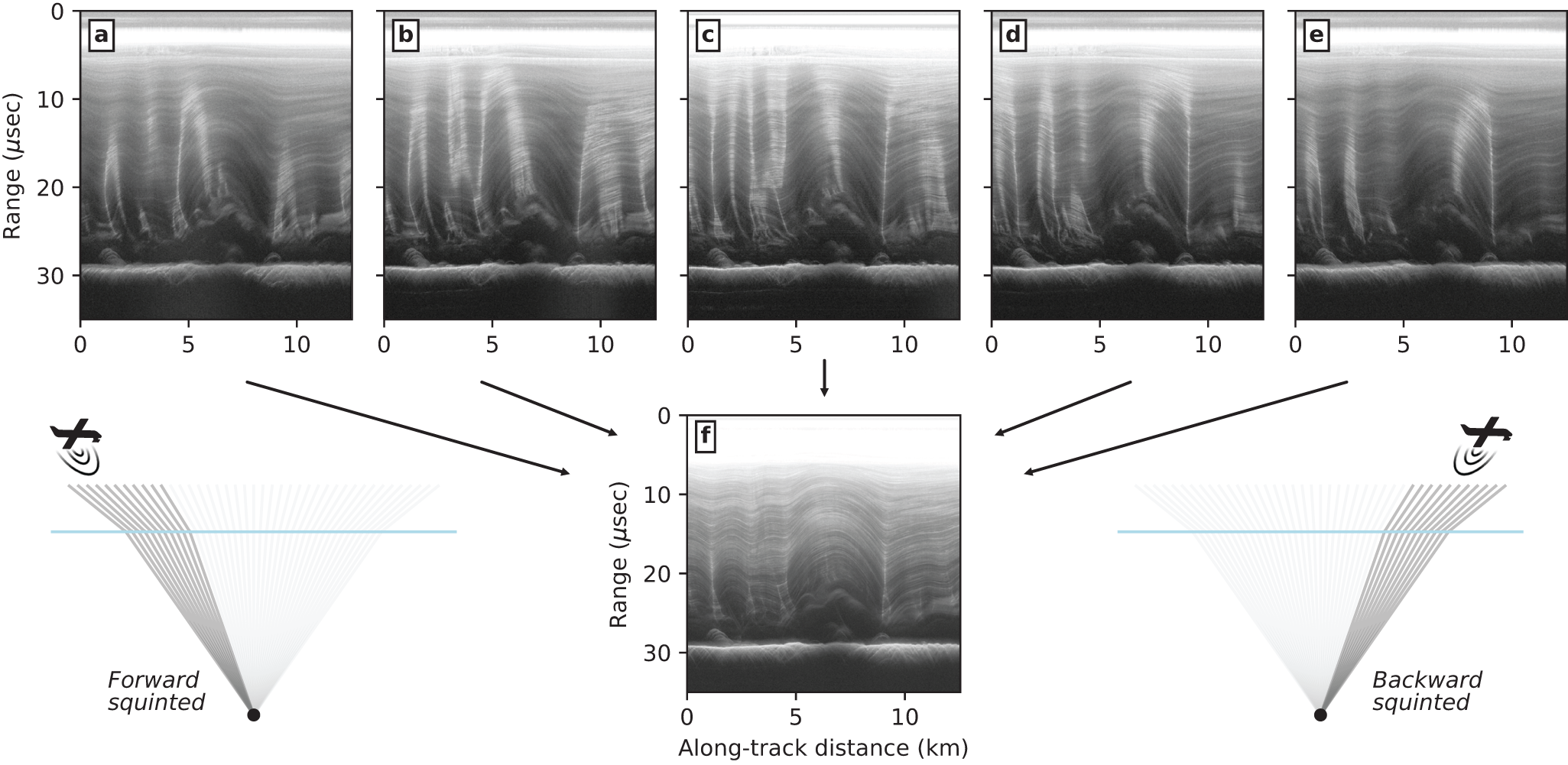
Figure 4. Results from multi-squinting, again using the same data segment as in Figs. 2 and 3. Individual images processed with one squinted subaperture, with (a, b) forward, (c) nadir, and (d, e) backward look angles. The nadir-squinted subaperture is the same nadir-focused image as in Fig. 3a. (f) The mosaic image, which is an incoherent average of all squinted subapertures in panels (a–e) and six additional subapertures at higher Doppler frequencies not shown here, for a total of 11 distinct squint angles. Illustrations on either side of the final mosaic image show cartoon examples of the forward- and backward-squinted subaperture geometries.
In our implementation of squinted subaperture processing, we offset squint angles by one-half the subaperture width so that each overlaps with its neighbor (Fig. 4a–e), then convolved with a Hanning window in Doppler space so that the total power is conserved. Finally, the subapertures are incoherently averaged (multilooked) to create the mosaic in which both specular and diffuse targets can be resolved across the Doppler spectrum (Fig. 4f). Note that specular targets may exhibit a drop in SNR relative to the original nadir-focused image since we are now averaging over more measurements through the full Doppler spectrum, most of which are noise in the case of a specular target. This is true of both the multi-squinted algorithm and simple resampling, as can be seen in Fig. 3, where the targets that are resolved in Fig. 3a have a slight power reduction with resampling in Fig. 3b and c.
3.2. Adaptive squinting and spectral filtering
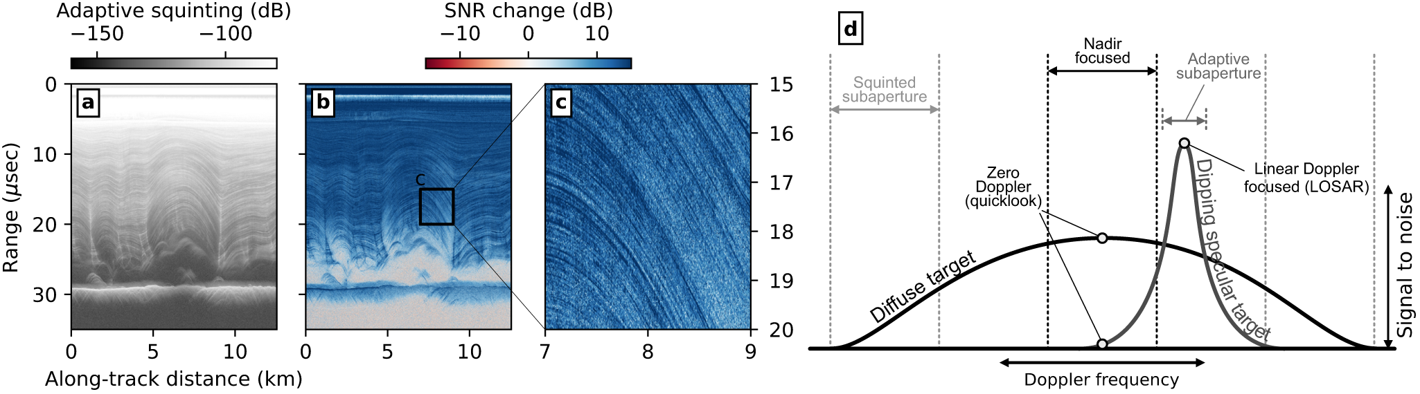
Next, consider an adaptive subaperture, one that is restricted to the portion of the Doppler spectrum with signal above the noise floor (Fig. 5). Here, we increase the number of squinted subapertures, enough that Doppler space can be treated as its own dimension (with the many small subapertures as Doppler bins) to be analyzed and filtered. We then iterate through each pixel in the image, applying a Tukey filter in Doppler space to suppress noise at high Doppler frequencies and again identifying the Doppler centroid as the bin with the greatest SNR. From the centroid, we progressively step outward, including bins until they fall below a prescribed SNR threshold (in this case, within 10 dB of the system noise floor, which is defined by range bins well below the deepest targets, or any possible clutter,  $\sim$40 $\mu$sec). To maintain a continuous aperture and to restrictively limit its extent, we do not include any additional bins after the first is rejected (i.e., the lowest frequency bin that falls below the threshold is the aperture extent). In the limit where the adaptive aperture is confined to a single frequency at the Doppler centroid, our adaptive approach reduces to the linear-Doppler focusing method described above (Castelletti and others, Reference Castelletti, Schroeder, Mantelli and Hilger2019).
Since this adaptive focusing method removes the Doppler bins with low signal, which were averaged into previous results, the overall SNR is elevated, especially for specular reflectors that have a narrow response in Doppler space (Fig. 5b and c). However, the method is computationally expensive compared to those approaches with a fixed number of (sub)aperture(s). A similar and faster approach would be to apply spectral filtering (Heister and Scheiber, Reference Heister and Scheiber2018) on an image that has already been focused with one of the methods above, but in that case, the focused image may have already destructively interfered signals, and therefore have diminished SNR for dipping layers. In those cases, layers will be more recoverable with a low-level adaptive aperture as we describe here compared to higher-level filtering.

Figure 5. A signal-to-noise ratio (SNR) improvement through adaptive squinting. (a) The resulting image from adaptive squinting, (b) the SNR difference of adaptive squinting compared to multi-squinting across the full Doppler bandwidth (i.e., Fig. 4f) and (c) an inset of the difference to better highlight the SNR improvement for specular, dipping englacial layers. (d) Conceptual diagram of englacial targets (diffuse and specular) as they are represented in Doppler space and how they are sampled through different processing types or (sub)apertures.
4. Application at Academy Glacier
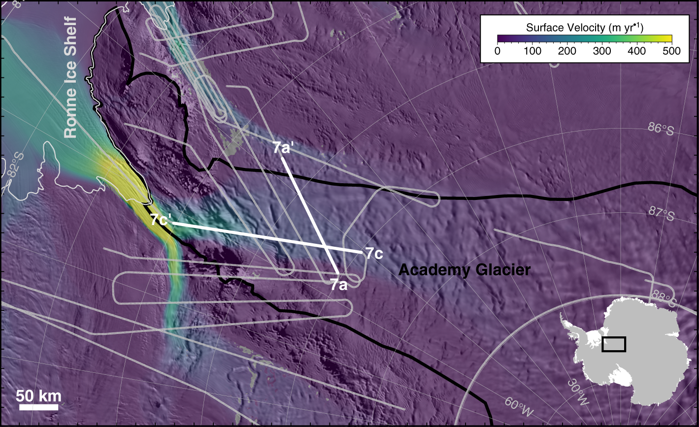
We apply the above methodology to selected segments of an Operation IceBridge airborne radar survey flown by the Center for Remote Sensing and Integrated Systems (CReSIS) in October and November of 2018 (Fig. 6). For this survey, the Multi-channel Coherent Radar Depth Sounder 3 (MCoRDS3) (Rodriguez-Morales and others, Reference Rodriguez-Morales2013), with a six-element antenna-array, was mounted in the cross-track direction under a DC8 airframe and operated across a 165–215 MHz frequency band. The surveyed area included both along- and across-flow (flux-gate) profiles for glaciers in the Filchner Ice Shelf drainage basin, East Antarctica. Here, we emphasize two profiles in particular from Academy Glacier.

Figure 6. A map of the airborne radar survey flown by CReSIS in 2018, overlain on the observed surface velocities (Mouginot and others, Reference Mouginot, Rignot and Scheuchl2019) and MODIS imagery Scambos and others (Reference Scambos, Haran, Fahnestock, Painter and Bohlander2007). The Academy Glacier drainage basin is outlined in black (Rignot and others, Reference Rignot, Mouginot and Scheuchl2011) and the grounding line in white (Depoorter and others, Reference Depoorter2013).
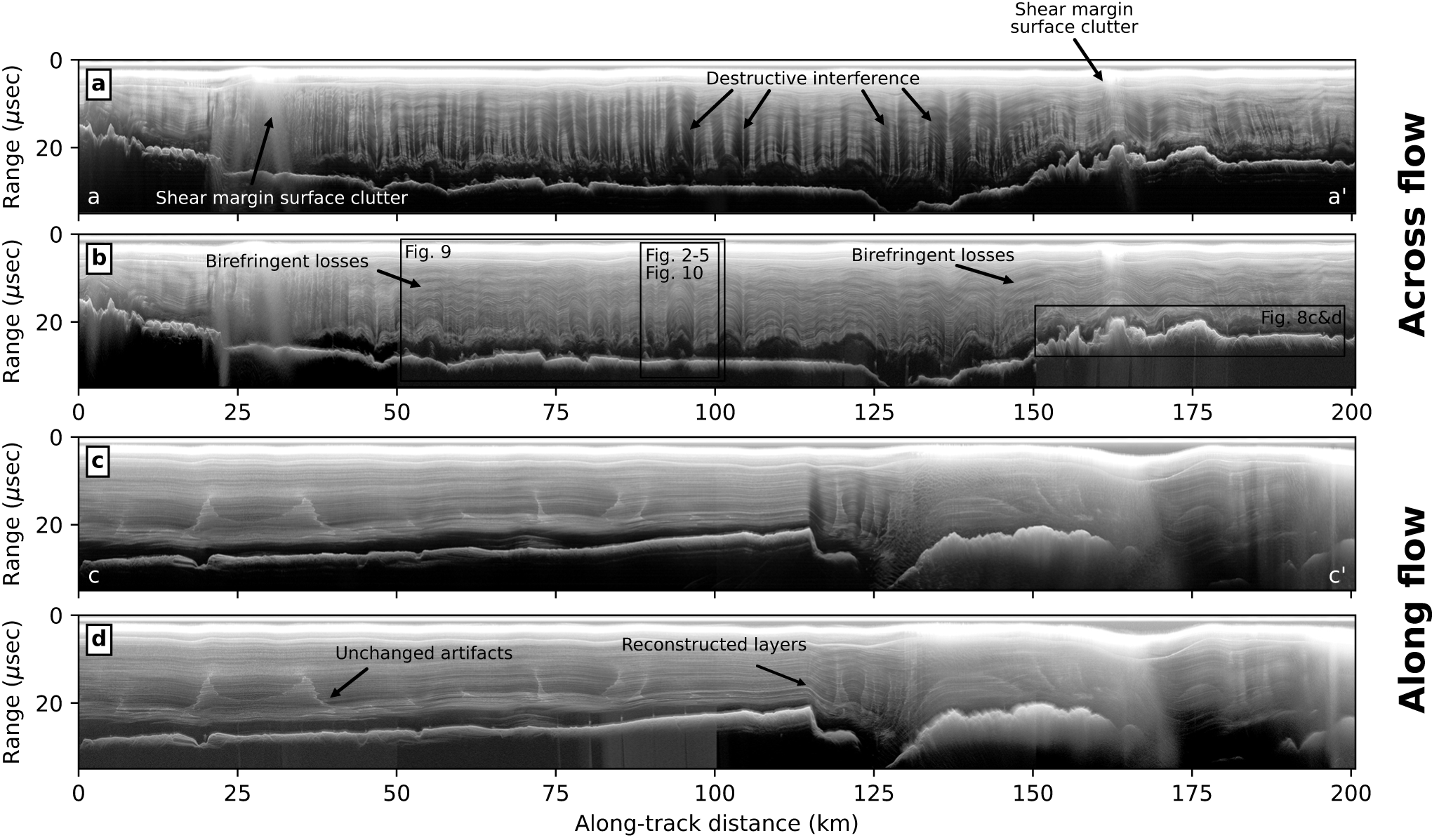
Academy Glacier is a part of the broader Foundation-Patuxent-Academy ice-stream system (Ross and others, Reference Ross2025), being closely coupled to neighboring Foundation and Support Force ice streams. The upstream accumulation area, in the vicinity of the South Pole, overlies the large Pensacola-Pole bedrock basin (Paxman and others, Reference Paxman2019), and accumulated ice from that basin is funneled through the Pensacola Mountains by Academy Glacier. Cross-glacier convergence creates folding in the englacial stratigraphy (Bons and others, Reference Bons2016), which causes destructive interference within radar images of dipping layers (Fig. 7a) for the reasons discussed above. Those dipping layers are effectively reconstructed with squinted SAR processing (Fig. 7b), indicating that the dominant dip angle is in line with the flight track (perpendicular to the flow direction). After layer reconstruction, alternative mechanisms of radar power reduction become more apparent; for example, there is a birefringent beat signature (Young and others, Reference Young2021; Hills and others, Reference Hills2025) at 55 km and 150 km along-track distances, near the lateral extent of streaming flow. In the along-flow direction, Academy Glacier has a retrograde bedslope (Jeofry and others, Reference Jeofry2018) before it drops into Foundation Trough. The along-flow radiostratigraphy is relatively uniform and flat overlying the retrograde bed, but some artifacts are present in the radar image (Fig. 7c). Since those features are not suppressed by squinted focusing (Fig. 7d), we assume they are cross-track layer folds (see Section 5.2), consistent with what is observed in the cross-flow profile.

Figure 7. Radar profiles from the 2018 Operation IceBridge survey of Academy Glacier aligned (a, b) across and (c, d) along ice flow using (a, c) conventional nadir-focused and (b, d) our adaptively squinted processing, each with color scales in dB relative to their noise floor. The cross-flow profile is aligned such that ice is flowing into the page. Most of the destructive interference in the cross-flow profile, which is from dipping englacial layers in panel (a), can be recovered, as shown in panel (b). The along-flow profile is aligned such that ice is flowing left to right. Constructively interfered vertical artifacts in the first 100 km of the along-flow profile are unchanged in the squinted image, indicating that they are associated with cross-track layer dips. Some Doppler-filtering artifacts arise in the squinted processing (e.g., panel (d) within 75–100 km and below the bed interface), which could be mitigated appropriately with adjustments to the applied Tukey window. Steeply dipping layers from 115 km to 125 km are successfully reconstructed with our squinted subaperture processing.
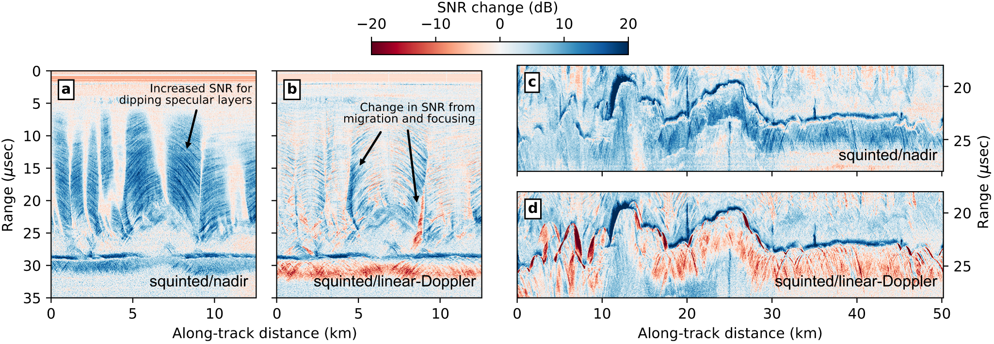
Even for features which are well resolved with standard focusing (e.g., the ice-bed interface), the resulting SNR changes substantially between focusing methods (Fig. 8). Methods with a large Doppler bandwidth tend to average in more noise and increase the noise floor, but they do so while resolving specular reflectors from all dip angles equally (as opposed to fading in and out of the nadir image). The adaptive aperture minimizes this additional noise to the point where SNR for flat layers is at least equal to nadir focusing (or greater for large nadir apertures) and SNR for dipping layers is elevated to match those that are flat (Fig. 8a and c). The trailing tail beneath a bed echo and clutter from surface crevassing can be intensified relative to the nadir image since this energy is associated with diffuse reflections from off-nadir topography (as opposed to the initial bed- or surface-echo impulse associated with scattering at nadir). Compared to the linear-Doppler image (Fig. 8b and d), adaptive-squinting has lower SNR for some targets, especially those that are highly specular, but now with more ability to accommodate changes in layer shape through range migration and non-linear focusing.

Figure 8. SNR difference between focusing methods for (a, b) the same cross-flow profile segment shown in Figs. 2 –5 with specular englacial layers, and (c, d) a different segment of the same cross-flow profile with diffuse bed echoes (location shown in Fig. 7b). (a, c) Difference between adaptive squinting and nadir-focused images. (b, d) Difference between adaptive squinting and linear-Doppler processed images.
5. Discussion
Englacial stratigraphy has commonly been used to infer ice flow and ice-sheet history, including in past studies at Academy Glacier (e.g., Bingham and others, Reference Bingham, Siegert, Young and Blankenship2007; Sanderson and others, Reference Sanderson2024). In cases where layer folds and/or disruptions are spatially consistent with the measured velocities at the ice-sheet surface, ice flow has been interpreted to be in a steady state (e.g., Martín and others, Reference Martín, Gudmundsson and King2014). Alternatively, in cases where the two measures are inconsistent, historical changes to ice flow have been interpreted (e.g., Conway and others, Reference Conway, Catania, Raymond, Gades, Scambos and Engelhardt2002; Karlsson and others, Reference Karlsson, Rippin, Vaughan and Corr2009), and in some cases an approximate timing has been assigned to the change (e.g., Beem and others, Reference Beem2017; Hoffman and others, Reference Hoffman, Summers, Suckale, Christianson, Catania and Conway2025). As we have shown, the degree to which layers appear disrupted also depends on the processing methodology. In this section, we discuss how the different SAR processing methods may or may not affect interpretations of the stratigraphy and how additional analyses may be possible with our new data product(s).
5.1. Layer continuity
Radiostratigraphy can be analyzed by discrete interpretation of individual layers (MacGregor and others, Reference MacGregor2015); however, depending on the goal, it can be simpler and faster to quantify abnormalities on a trace-by-trace basis, for instance, with an A-scope continuity index (Karlsson and others, Reference Karlsson, Rippin, Bingham and Vaughan2012)
 \begin{equation}
\Psi = \frac{1}{2\Delta z N} \sum_{i=n_1}^{n_N} |P_{i+1}-P_{i-1}|
\end{equation}
\begin{equation}
\Psi = \frac{1}{2\Delta z N} \sum_{i=n_1}^{n_N} |P_{i+1}-P_{i-1}|
\end{equation} where  $\Delta z$ is the vertical distance, in meters, between range bins, $N$ is the number of range bins included in the sum (generally restricted to some subset of the total ice thickness) and $P$ is the radar power (or SNR) at a given range bin,
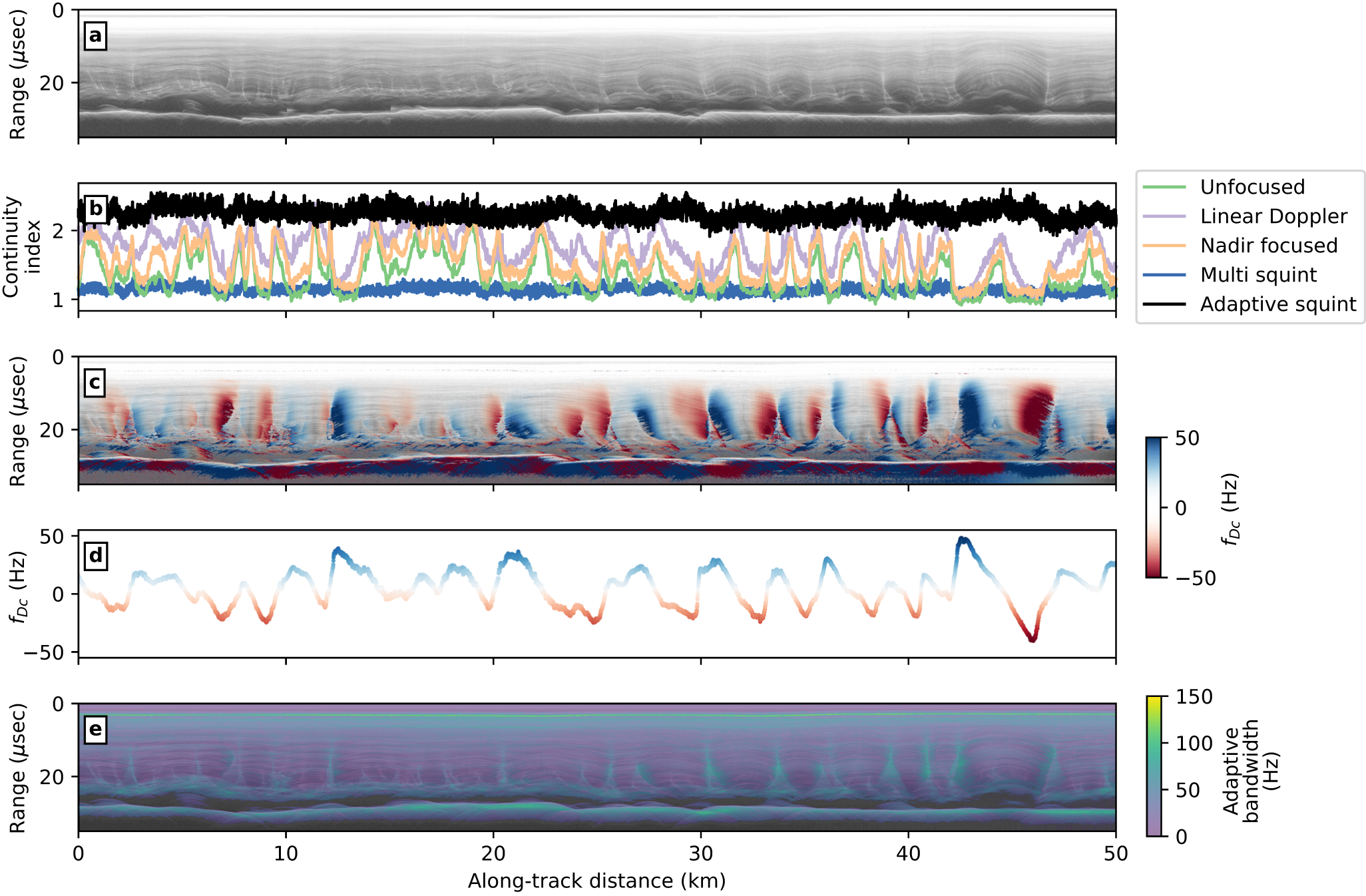
  $i$. We calculated the continuity index for layers within the same radar image from the cross-flow segment of Academy Glacier (Fig. 9a; location in Fig. 7b) processed five ways: unfocused, linear-Doppler focused, nadir focused, multi-squint focused and adaptive-squint focused (Fig. 9b). In the three more commonly applied data products, destructive interference in dipping layers is associated with a drop in the continuity index, whereas the adaptively squinted image has relatively continuous layers throughout. The multi-squinted image has a lower continuity index everywhere, but this is due to how the index is calculated, not that the layers are not resolved continuously. That is, the multi-squinted image has higher noise, so the contrast between the noise floor and the reflection SNR is smaller and therefore the vertical gradient calculation in equation 7 is smaller everywhere. Aside from two slight dips in continuity at the most steeply dipping layers ( $\sim$42 and 45 km along track), the variations in continuity for the multi- and adaptively squinted images are not interpretable above the noise of layer reflectivities.

Figure 9. Comparison of layer continuity between processing techniques. (a) Adaptively squinted image from across Academy Glacier (location in Fig. 7b). (b) Layer continuity calculated with equation (7) for the profile section in (a), processed with all methods from Fig. 2 as well as the multi- and adaptively squinted techniques. (c) Doppler centroids overlain on the unfocused Doppler image. (d) Depth-averaged Doppler centroid. (e) Adaptive Doppler bandwidth, which can be used as a measure of specularity.
As one alternative to layer continuity, the Doppler centroids can be used to estimate layer dip (Arenas-Pingarrón and others, Reference Arenas-Pingarrón2025) (Fig. 9c and d). Then, there is a sign (up- or down-dipping) associated with the layers. Similar work has done the same layer-dip estimation, even for radars that are not phase coherent, through alternative image processing techniques (Panton, Reference Panton2014; Holschuh and others, Reference Holschuh, Parizek, Alley and Anandakrishnan2017; Delf and others, Reference Delf, Schroeder, Curtis, Giannopoulos and Bingham2020), but with less capability to recover the stratigraphy itself. The Doppler centroid can also be used to guide explicit tracking of individual layers (MacGregor and others, Reference MacGregor2015, their Fig. 3).
5.2. Cross-track layer folds
The along-track resampling and squinted steering methodology discussed here is useful for resolving radiostratigraphy that dips in the along-track direction. However, englacial stratigraphy is three-dimensional and therefore commonly has some cross-track dipping component as well. Multi-element antenna arrays are increasingly being used for cross-track beam steering (Paden and others, Reference Paden, Akins, Dunson, Allen and Gogineni2010) and swath mapping of off-nadir cross-track reflections (e.g., Holschuh and others, Reference Holschuh, Christianson, Paden, Alley and Anandakrishnan2020; Hoffman and others, Reference Hoffman2023). In theory, a multi-element array or a gridded survey enables a measurement for three-dimensional dip angle (similar to the Doppler centroid, but in the cross-track direction as well).
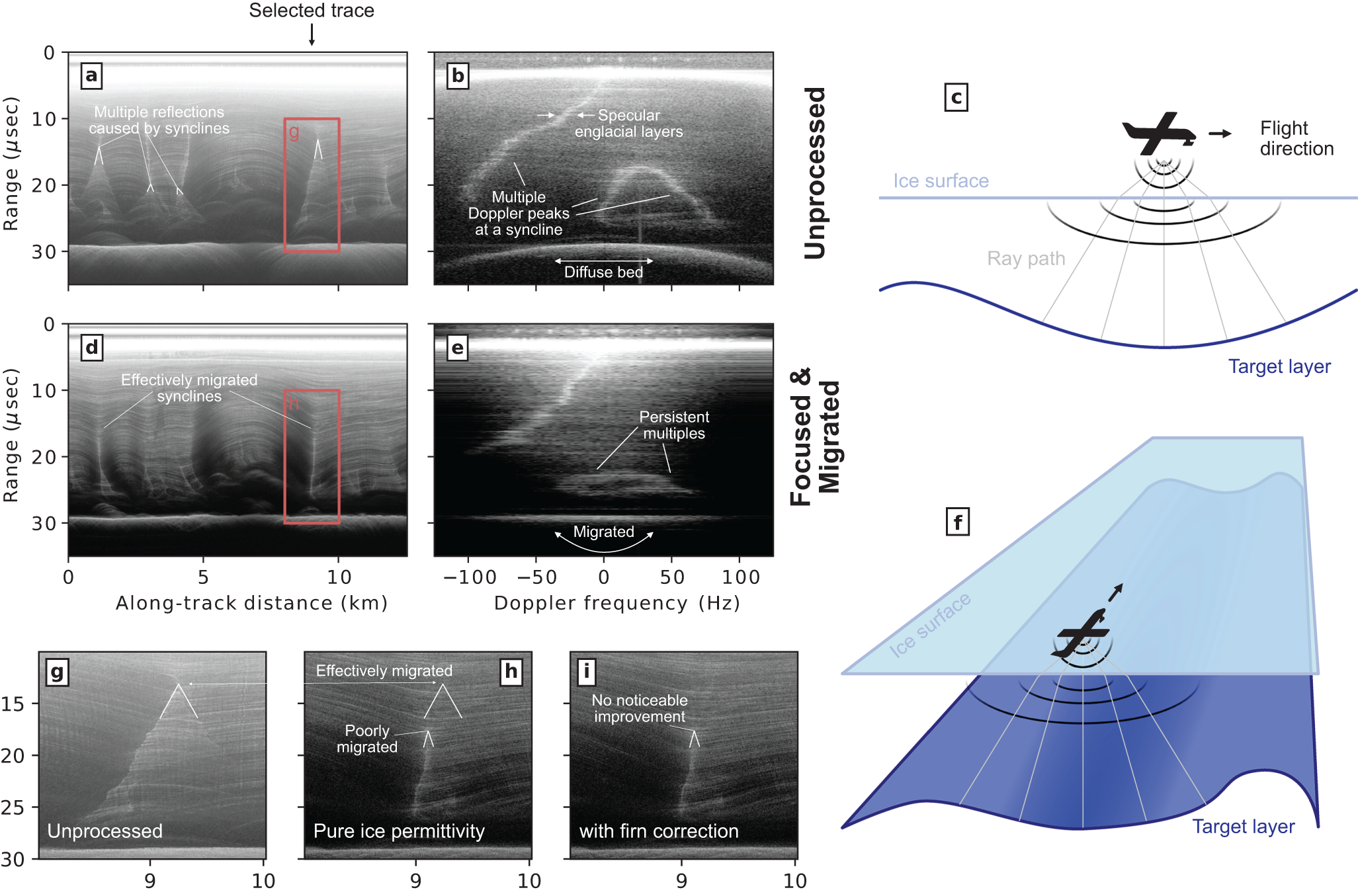
Although that is beyond the scope of this article, we can identify features in the along-track image which are not well resolved with along-track focusing, even with our improved methodology, and argue that they are likely associated with interference from cross-track reflections, with some shape out of the plane of the image (not necessarily perfectly orthogonal) (Fig. 10). To do so, we first point out that synclines (i.e., concave up layers or sets of layers) can lead to multiple peaks within one range row of the Doppler spectrum of the unfocused along-track image (Fig. 10a and b) if the same layer lies on multiple points of equal range from the radar instrument (Fig. 10c). These multiple reflections create a downward cone of anomalous stratigraphy in the unfocused image, which is migrated away with focusing if the syncline is positioned in line with the profile (Fig. 10d and e). However, since the focusing is along the flight track only, it does not migrate any cross-track features and those artifacts in the unfocused image are then persistent into the focused one. Anomalously high power in the focused image may then indicate some analogous syncline in the cross-track direction (Fig. 10f), especially if more careful focusing (e.g., with a firn correction for permittivity) does not improve the migration (Fig. 10g–i).

Figure 10. Doppler analysis before and after range migration and focusing. (a) Pulse-compressed image as in Fig.2a. (b) Doppler spectra from the pulse-compressed image at the selected trace location indicated in (a). (c) Illustration of an along-track concave up layer which creates multiple reflections with the same range. (d) Resampled (to 0.5 m spacing) and focused image as in Fig. 3c. (e) Doppler spectra after focusing to demonstrate the effect of migration on subsurface targets. (f) Illustration of a cross-track syncline. Three panels show a smaller inset image for: (g) pulse compressed; (h) focused; and (i) focused with a firn-density correction. The multiple reflections that are effectively migrated are associated with an along-track syncline, and those that are poorly migrated are associated with a cross-track syncline.
5.3. Specularity
Englacial layers are typically specular, especially compared to the ice-bed interface. A measure of specularity can be calculated from the Doppler spectra, where a narrow Doppler peak indicates a specular reflector and a wide Doppler peak indicates a diffuse reflector (Fig. 10b). For instance, past studies on specularity have used the difference in coherent power between apertures of different sizes (e.g., Schroeder and others, Reference Schroeder, Blankenship and Young2013; Young and others, Reference Young, Schroeder, Blankenship, Kempf and Quartini2016), with the wider aperture having lower SNR for specular reflectors because it stacks in more noise from portions of the Doppler spectra outside what is reflected by the target. Those analyses have typically been used to characterize the ice-bed interface; for instance, because a wet bed, and especially a subglacial lake, is expected to be more specular than a dry bed or one with significant subglacial roughness (e.g., Chu and others, Reference Chu2021; Haris and others, Reference Haris, Chu and Robel2024). Such a two-aperture comparison works particularly well for nadir targets, but dipping specular targets may have higher SNR in the wider aperture if the narrower aperture did not appropriately resolve the target.
Our adaptive aperture processing accommodates dipping targets, so it can also yield a more robust specularity estimate based on the selected bandwidth of the adaptive aperture. A narrow bandwidth is associated with a specular target and wide with diffuse, as can be seen in Fig. 9e where the bed has a larger adaptive bandwidth than the englacial layers. One notable exception is that the syncline features discussed before have a large adaptive bandwidth because of their multiple peaks in Doppler space, which all need to be included across the aperture. Taking these adaptive-aperture bandwidths, they can be used as their own data product in the same way that the Doppler centroids can be. Expanded use cases from previous the specularity estimates (e.g., Schroeder and others, Reference Schroeder, Blankenship and Young2013; Young and others, Reference Young, Schroeder, Blankenship, Kempf and Quartini2016) are predominantly for dipping targets which are not centered on zero Doppler. For example, one could use this methodology to examine the scattering effects of entrained material in basal ice (e.g., Winter and others, Reference Winter2019; Hills and others, Reference Hills, Siegfried and Schroeder2024) or hypothesize formation mechanisms for the echo-free zone and basal units (e.g., Yan and others, Reference Yan2025; Young and others, Reference Young2025).
6. Summary
In this work, we described how SAR processing can be optimally used to resolve along-track dips within the englacial radiostratigraphy, for which the destructive interference has long been a topic of interest in the glaciology literature (e.g., Karlsson and others, Reference Karlsson, Rippin, Vaughan and Corr2009; Holschuh and others, Reference Holschuh, Christianson and Anandakrishnan2014, Reference Holschuh, Parizek, Alley and Anandakrishnan2017; Castelletti and others, Reference Castelletti, Schroeder, Mantelli and Hilger2019). Improved resolution of folded englacial layers can lead to superior and more robust radioglaciological interpretations; for example, of snow accumulation (Medley and others, Reference Medley2013), ice dynamics in the accumulation zone (e.g., near a Raymond Arch; Martín and others, Reference Martín, Gudmundsson and King2014), dynamics in streaming ice (Jansen and others, Reference Jansen2024) and paleo ice flow (Conway and others, Reference Conway, Catania, Raymond, Gades, Scambos and Engelhardt2002). Two additional analyses are necessarily calculated in our SAR methodology and optionally output as separate data products from the main radar image, layer dip through the Doppler centroid and specularity through the adaptive Doppler bandwidth. We also showed that derived data products from radiostratigraphy, such as a layer continuity index, are strongly dependent not only on the higher-level signal extraction approach but also on the lower-level SAR processing methods. Additional and more detailed analyses may be possible in areas with complex radiostratigraphy, even with RES data from previous missions, by using squinted focusing methods to illuminate englacial targets.
Data and software
All radar processing for the figures in this article was done with Open Polar Radar (2024). Processed data products are available at (Hills, Reference Hills2025b). The radar dataset used throughout was collected by the Center for Remote Sensing and Integrated Systems, with support from the University of Kansas, NASA grants 80NSSC20K1242 and 80NSSC21K0753, and NSF grants OPP-2027615, OPP-2019719, OPP-1739003, IIS-1838230, RISE-2126503, RISE-2127606 and RISE-2126468.
An additional Python-based squinted SAR algorithm is available at https://github.com/benhills/squintsar with a frozen version (Hills, Reference Hills2025a).
Acknowledgements
We thank the scientific editor, Michelle Koutnik, and two anonymous reviewers for the revisions they offered on an earlier draft of this article. Ian Joughin, Riley Culberg, John Paden and Jilu Li also provided valuable input through conversations on the topics presented herein.
Funding
This work was primarily funded by an NSF Postdoctoral Research Fellowship through the Office of Polar Programs (award number 2317927). HV was funded by an NSF Graduate Research Fellowship (award number 2137099). HV and MRS were also supported by NSF grant 2049302.
Conflicts of interest
The authors declare no conflicts of interest.


 Open access