


1. Introduction
In [Reference ZagierZag10], Zagier introduced the concept of quantum modular forms (QMF). Given a Fuchsian cofinite subgroup
 $\Gamma$
of
$\Gamma$
of
 $\textrm{SL}(2, \mathbb{Z})$
whose set of cusps
$\textrm{SL}(2, \mathbb{Z})$
whose set of cusps
 $C(\Gamma)\subset \mathbb{P}^1(\mathbb{Q})$
is non-empty, and
$C(\Gamma)\subset \mathbb{P}^1(\mathbb{Q})$
is non-empty, and
 $k\in\mathbb{C}$
, QMF are defined as functions
$k\in\mathbb{C}$
, QMF are defined as functions
 $$f : C(\Gamma)\smallsetminus S \to \mathbb{C},$$
for some finite set S, satisfying a form of modularity, in the purposely vague sense that for any
 $\gamma=(\begin{smallmatrix}a & b\\ c&d\end{smallmatrix})\in\Gamma$
, the period function
$\gamma=(\begin{smallmatrix}a & b\\ c&d\end{smallmatrix})\in\Gamma$
, the period function
 \begin{align} h_\gamma(x):= f(x) - |cx+d|^{-k}f\bigg(\frac{ax +b}{cx+d}\bigg),\quad x\in C(\Gamma)\smallsetminus (S\cup \gamma^{-1}S)\end{align}
is somewhat regular with respect to the real topology. The exact assumptions vary widely in the literature; in our case, we will mainly require continuity or bounds on the growth around possible singularities.
Numerous examples of quantum modular forms are known, in various contexts, and we refer in particular to [Reference ZagierZag10, Reference Bringmann, Folsom and RhoadesBFR15, Reference Ngo and RhoadesNR17, Reference Kim, Lim and LovejoyKLL16, Reference Bruggeman, Lewis and ZagierBLZ15, Reference Marmi, Moussa and YoccozMMY97, Reference Jaffard and MartinJM18]. More references are listed in the introduction of [Reference Bettin and DrappeauBD22].
In this paper, we focus on QMF for the full modular group
 $\Gamma =\textrm{SL}(2, \mathbb{Z})$
, so that
$\Gamma =\textrm{SL}(2, \mathbb{Z})$
, so that
 $C(\Gamma) =\mathbb{P}^1(\mathbb{Q})$
, and which are periodic (i.e.
$C(\Gamma) =\mathbb{P}^1(\mathbb{Q})$
, and which are periodic (i.e.
 $h_{U}=0$
for
$h_{U}=0$
for
 $U=(\begin{smallmatrix}1 & 1\\ 0&1\end{smallmatrix})$
).Footnote
1
By composition, it is sufficient to consider (1.1) for the second generator
$U=(\begin{smallmatrix}1 & 1\\ 0&1\end{smallmatrix})$
).Footnote
1
By composition, it is sufficient to consider (1.1) for the second generator
 $\gamma=(\begin{smallmatrix}0 & -1\\ 1&0\end{smallmatrix})$
of
$\gamma=(\begin{smallmatrix}0 & -1\\ 1&0\end{smallmatrix})$
of
 $\textrm{SL}(2, \mathbb{Z})$
, so that, in order to prove that f is a QMF, one only needs to verify that
$\textrm{SL}(2, \mathbb{Z})$
, so that, in order to prove that f is a QMF, one only needs to verify that
 \begin{align} h(x):= f(x) - |x|^{-k}f(-1/x)\quad (x\in\mathbb{Q}\smallsetminus\{0\})\end{align}
has some regularity property.
The cases of
 $\operatorname{Re}(k)=0$
and
$\operatorname{Re}(k)=0$
and
 $\operatorname{Re}(k)\neq0$
are different in nature. In the case
$\operatorname{Re}(k)\neq0$
are different in nature. In the case
 $k=0$
, by iterating the relation (1.2) and using periodicity, we can express f as a twisted Birkhoff sum of h evaluated along orbits under the Gauss map, see [Reference Bettin and DrappeauBD22, Equation (3.1)], the twist being given by the multiplicative automorphic factor. Using this observation, in [Reference Bettin and DrappeauBD22] it was then shown that, for a large class of functions h, the multisets
$k=0$
, by iterating the relation (1.2) and using periodicity, we can express f as a twisted Birkhoff sum of h evaluated along orbits under the Gauss map, see [Reference Bettin and DrappeauBD22, Equation (3.1)], the twist being given by the multiplicative automorphic factor. Using this observation, in [Reference Bettin and DrappeauBD22] it was then shown that, for a large class of functions h, the multisets
 $\{f(x)\mid x\in\mathbb{Q}\cap[0,1),\, \operatorname{Den}(x)\leqslant Q\}$
become asymptotically distributed, as
$\{f(x)\mid x\in\mathbb{Q}\cap[0,1),\, \operatorname{Den}(x)\leqslant Q\}$
become asymptotically distributed, as
 $Q\to\infty$
, according to a stable law, which is in fact a normal law if h is of moderate growth at 0.Footnote
2
As a consequence, one has that, in general, f is nowhere continuous according to the real topology, nor can f be extended by continuity to any point outside of
$Q\to\infty$
, according to a stable law, which is in fact a normal law if h is of moderate growth at 0.Footnote
2
As a consequence, one has that, in general, f is nowhere continuous according to the real topology, nor can f be extended by continuity to any point outside of
 $\mathbb{Q}$
. For the same reasons, we expect a similar phenomenon to occur whenever
$\mathbb{Q}$
. For the same reasons, we expect a similar phenomenon to occur whenever
 $\operatorname{Re}(k)=0$
.
$\operatorname{Re}(k)=0$
.
The purpose of the present paper is to study the case when
 $\operatorname{Re}(k)\neq 0$
.
$\operatorname{Re}(k)\neq 0$
.
1.1 Weights with negative real parts
If
 $\operatorname{Re}(k)<0$
and h is continuous on
$\operatorname{Re}(k)<0$
and h is continuous on
 $[-1,1]\smallsetminus \{0\}$
with finite right and left limits
$[-1,1]\smallsetminus \{0\}$
with finite right and left limits
 $h(0^\pm)$
at 0, then we show that, in fact, f can always be extended by continuity to a bounded function
$h(0^\pm)$
at 0, then we show that, in fact, f can always be extended by continuity to a bounded function
 $f^\triangleleft:\mathbb{R}\to\mathbb{C}$
. Moreover, we prove that
$f^\triangleleft:\mathbb{R}\to\mathbb{C}$
. Moreover, we prove that
 $f^\triangleleft$
is continuous on
$f^\triangleleft$
is continuous on
 $\mathbb{R}\smallsetminus \mathbb{Q}$
and is continuous on the whole real line if
$\mathbb{R}\smallsetminus \mathbb{Q}$
and is continuous on the whole real line if
 $h(0\pm)=f(0)$
, a condition that could be morally interpreted as saying that (1.2) holds also at ‘
$h(0\pm)=f(0)$
, a condition that could be morally interpreted as saying that (1.2) holds also at ‘
 $0^{\pm}$
’. More precisely, the following holds.
$0^{\pm}$
’. More precisely, the following holds.
Theorem 1.1. Let
 $\operatorname{Re}(k)<0$
and let
$\operatorname{Re}(k)<0$
and let
 $f:\mathbb{Q}\to\mathbb{C}$
be a 1-periodic function satisfying (1.2) for a function
$f:\mathbb{Q}\to\mathbb{C}$
be a 1-periodic function satisfying (1.2) for a function
 $h:\mathbb{R}\smallsetminus \{0\}\to \mathbb{C}$
which is continuous on
$h:\mathbb{R}\smallsetminus \{0\}\to \mathbb{C}$
which is continuous on
 $[-1,1]\smallsetminus \{0\}$
with finite left and right limits
$[-1,1]\smallsetminus \{0\}$
with finite left and right limits
 $h(0^\pm)$
at 0. Then the function
$h(0^\pm)$
at 0. Then the function
 \begin{align} f^\triangleleft(x):= \begin{cases} f(x) & \text{if }x\in\mathbb{Q},\\ {\displaystyle \lim_{\mathbb{Q}\ni y\to x}f(y)} & \text{if }x\notin\mathbb{Q} \end{cases} \end{align}
is defined for all
 $x\in\mathbb{R}$
and is continuous on
$x\in\mathbb{R}$
and is continuous on
 $\mathbb{R}\smallsetminus\mathbb{Q}$
. Moreover, for any rational
$\mathbb{R}\smallsetminus\mathbb{Q}$
. Moreover, for any rational
 $x= a/q$
in reduced form, one has
$x= a/q$
in reduced form, one has
 $f^\triangleleft(y)\to f(x) + q^k(h(0^\pm)-f(0))$
as
$f^\triangleleft(y)\to f(x) + q^k(h(0^\pm)-f(0))$
as
 $y\to x^\pm$
. In particular,
$y\to x^\pm$
. In particular,
 $f^\triangleleft$
is continuous on
$f^\triangleleft$
is continuous on
 $\mathbb{R}$
if and only if
$\mathbb{R}$
if and only if
 $h(0^\pm)=f(0)$
. Furthermore, in this case, if
$h(0^\pm)=f(0)$
. Furthermore, in this case, if
 $h\in\mathcal C^{m}([-1,1],\mathbb{C})$
with
$h\in\mathcal C^{m}([-1,1],\mathbb{C})$
with
 $0\leqslant m < {| {\operatorname{Re}(k)} |}/2$
, then
$0\leqslant m < {| {\operatorname{Re}(k)} |}/2$
, then
 $f^\triangleleft\in\mathcal C^{m}(\mathbb{R},\mathbb{C})$
.
$f^\triangleleft\in\mathcal C^{m}(\mathbb{R},\mathbb{C})$
.
If h is continuous at 0 but
 $h(0)\neq f(0)$
, we can modify f by letting
$h(0)\neq f(0)$
, we can modify f by letting
 $\widetilde f(x):=f(x)+\operatorname{Den}(x)^k(h(0)-f(0))$
. The map
$\widetilde f(x):=f(x)+\operatorname{Den}(x)^k(h(0)-f(0))$
. The map
 $\widetilde f$
is a QMF with h as its period function, and
$\widetilde f$
is a QMF with h as its period function, and
 $\widetilde f(0)=h(0)$
.
$\widetilde f(0)=h(0)$
.
As we will see below, in some of the examples of QMF that we will consider, the map f actually admits an expression as an absolutely converging Fourier series, and the differentiability of such series has been studied in detail in many instances, see in particular [Reference ChamizoCha04, Reference PetrykiewiczPet14, Reference Chamizo, Petrykiewicz and Ruiz-CabelloCPRC17]. Theorem 1.1 instead gives a proof of the continuity and differentiability of f extended to
 $\mathbb{R}$
which does not rely on an a priori knowledge of a Fourier expansion for f.
$\mathbb{R}$
which does not rely on an a priori knowledge of a Fourier expansion for f.
Theorem 1.1 shows that, in fact, one cannot expect the period function h to be continuous if f does not have some continuity property to start with, so that non-trivial instances of QMF (meaning those cases when h is more regular than f) arise only when h is differentiable at least
 $\lceil -\operatorname{Re}(k)/2\rceil$
times.
$\lceil -\operatorname{Re}(k)/2\rceil$
times.
Our method uses properties of the Gauss map, and is closely related to the works [Reference Marmi, Moussa and YoccozMMY97, Reference Lee, Marmi, Petrykiewicz and SchindlerLMPS24, Reference Balazard and MartinBM19]. These works are concerned with the regularity properties of the Brjuno function. This function is related to linearization problems in holomorphic dynamics [Reference BrjunoBrj72, Reference YoccozYoc88, Reference YoccozYoc95], and is close to being a QMF of weight
 $-1$
, see [Reference Marmi, Moussa and YoccozMMY06]. The methods of [Reference Marmi, Moussa and YoccozMMY97] likely extend to the setting of Theorem 1.1, and would be relevant to study e.g. the Hölder regularity of the highest-order derivative of f (see Definitions 1.1 to 1.3 in [Reference Chamizo, Petrykiewicz and Ruiz-CabelloCPRC17]).
$-1$
, see [Reference Marmi, Moussa and YoccozMMY06]. The methods of [Reference Marmi, Moussa and YoccozMMY97] likely extend to the setting of Theorem 1.1, and would be relevant to study e.g. the Hölder regularity of the highest-order derivative of f (see Definitions 1.1 to 1.3 in [Reference Chamizo, Petrykiewicz and Ruiz-CabelloCPRC17]).
We point out that precise estimates on Hölder regularity are achievable by methods from wavelet theory. In [Reference PetrykiewiczPet14] this was carried out using an explicit Fourier expansion, while in [Reference Jaffard and MartinJM18] instead this was performed using properties of the Gauss map, a point of view similar to the one taken in [Reference Marmi, Moussa and YoccozMMY97] or in the present paper.
The existence of the function
 $f^\triangleleft$
in (1.3) can actually be proved under much weaker hypotheses, which we explain in what follows. This will be required later on, when we will study cotangent sums.
$f^\triangleleft$
in (1.3) can actually be proved under much weaker hypotheses, which we explain in what follows. This will be required later on, when we will study cotangent sums.
Theorem 1.2. Suppose that
 $\operatorname{Re}(k)<0$
and let
$\operatorname{Re}(k)<0$
and let
 $\delta>0$
. Suppose that f satisfies
$\delta>0$
. Suppose that f satisfies
 \begin{equation} f(x) = f(x+1) \quad (x \in \mathbb{Q}\smallsetminus[-1, 0]), \end{equation}
in other words that f is 1-periodic separately on
 $(-\infty, 0)$
and
$(-\infty, 0)$
and
 $(0, \infty)$
, and that Equation (1.2) holds for
$(0, \infty)$
, and that Equation (1.2) holds for
 $x\in[-1, 1]\smallsetminus\{0\}$
, for a function h satisfying
$x\in[-1, 1]\smallsetminus\{0\}$
, for a function h satisfying
 \begin{align} \sup_{|x-y|<{e}^{-\varepsilon^{\delta-1}},\atop |x|>2\varepsilon} |h(x)-h(y)|=o(1)\quad \text{as }\varepsilon\to0^+,\quad h(x)=O({e}^{|x|^{\delta-1}})\quad \forall x\in[-1,1]\smallsetminus\{0\}. \end{align}
Then there is a full measure set
 $X \subset\mathbb{R}\smallsetminus\mathbb{Q}$
such that the limit
$X \subset\mathbb{R}\smallsetminus\mathbb{Q}$
such that the limit
 \begin{equation} f^\triangleleft(x) := \lim_{j\to\infty} f(x_j) \end{equation}
exists for
 $x\in X$
, where
$x\in X$
, where
 $(x_j) = ([a_0(x); a_1(x), \dotsc, a_j(x)])_j$
denotes the sequence of convergents of x. This value coincides with the limit (1.3) when h is bounded. In general, for any
$(x_j) = ([a_0(x); a_1(x), \dotsc, a_j(x)])_j$
denotes the sequence of convergents of x. This value coincides with the limit (1.3) when h is bounded. In general, for any
 $\varepsilon>0$
, there is a subset
$\varepsilon>0$
, there is a subset
 $X_\varepsilon\subset X$
invariant by
$X_\varepsilon\subset X$
invariant by
 $x\mapsto x+1$
and with
$x\mapsto x+1$
and with
 $\nu(X_\varepsilon \cap [0, 1]) \geqslant 1-\varepsilon$
, such that
$\nu(X_\varepsilon \cap [0, 1]) \geqslant 1-\varepsilon$
, such that
 $f^\triangleleft|_{X_\varepsilon}$
is continuous on
$f^\triangleleft|_{X_\varepsilon}$
is continuous on
 $X_\varepsilon$
equipped with the restricted topology. In particular,
$X_\varepsilon$
equipped with the restricted topology. In particular,
 $f^\triangleleft$
is Lebesgue-measurable.
$f^\triangleleft$
is Lebesgue-measurable.
The set X in this statement does not depend on f, h or
 $\delta$
. It consists of numbers having mildly growing continued fraction coefficients, see Lemma 2.2 below.
$\delta$
. It consists of numbers having mildly growing continued fraction coefficients, see Lemma 2.2 below.
The extension of the definition of f(x) also allows us to show that f has a limiting distribution when evaluated at reduced rationals
 $0\leqslant a/q<1$
with
$0\leqslant a/q<1$
with
 $q\to\infty$
.
$q\to\infty$
.
Theorem 1.3. Suppose that
 $\operatorname{Re}(k)<0$
and let
$\operatorname{Re}(k)<0$
and let
 $f:\mathbb{Q}\to\mathbb{C}$
satisfy (1.2) and (1.4), for a function
$f:\mathbb{Q}\to\mathbb{C}$
satisfy (1.2) and (1.4), for a function
 $h:\mathbb{R}\smallsetminus \{0\}\to \mathbb{C}$
satisfying (1.5). Then the multiset
$h:\mathbb{R}\smallsetminus \{0\}\to \mathbb{C}$
satisfying (1.5). Then the multiset
 $$ \{ f( a/q) \colon 1\leqslant a \leqslant q, (a, q)=1\} $$
becomes distributed, as
 $q\to \infty$
, according to the push-forward
$q\to \infty$
, according to the push-forward
 $ f^\triangleleft_\ast(\nu)$
of the Lebesgue measure
$ f^\triangleleft_\ast(\nu)$
of the Lebesgue measure
 $\nu$
on [0, 1] (see [Reference Le GallLG22, p. 13]).
$\nu$
on [0, 1] (see [Reference Le GallLG22, p. 13]).
If, moreover, h is real-analytic on
 $(-1, 1)\smallsetminus\{0\}$
and f is non-constant on
$(-1, 1)\smallsetminus\{0\}$
and f is non-constant on
 $\mathbb{Q}_{>0}$
, then the measure
$\mathbb{Q}_{>0}$
, then the measure
 $f^\triangleleft_\ast(\nu)$
is diffuse.
$f^\triangleleft_\ast(\nu)$
is diffuse.
In contrast with the case
 $k=0$
treated in [Reference Baladi and ValléeBV05, Reference Bettin and DrappeauBD22], we remark here that we did not need to perform an additional average over q in order to obtain a limiting statement.
$k=0$
treated in [Reference Baladi and ValléeBV05, Reference Bettin and DrappeauBD22], we remark here that we did not need to perform an additional average over q in order to obtain a limiting statement.
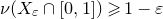
We recall that a measure is diffuse if it has no atoms. When
 $f^\triangleleft$
is real-valued, then
$f^\triangleleft$
is real-valued, then
 $f^\triangleleft_\ast(\nu)$
is supported on
$f^\triangleleft_\ast(\nu)$
is supported on
 $\mathbb{R}$
, and diffuseness is equivalent to the continuity of the associated cumulative distribution function. Under appropriate conditions, we are able to reach the stronger conclusion that for any non-zero linear form
$\mathbb{R}$
, and diffuseness is equivalent to the continuity of the associated cumulative distribution function. Under appropriate conditions, we are able to reach the stronger conclusion that for any non-zero linear form
 $\phi:\mathbb{C}\to\mathbb{R}$
, the measure
$\phi:\mathbb{C}\to\mathbb{R}$
, the measure
 $(\phi\circ f^\triangleleft)_\ast(\nu)$
on
$(\phi\circ f^\triangleleft)_\ast(\nu)$
on
 $\mathbb{R}$
is diffuse.Footnote
3
This is equivalent to the statement that the graph of
$\mathbb{R}$
is diffuse.Footnote
3
This is equivalent to the statement that the graph of
 $f^\triangleleft$
never remains on a given straight line for a positive proportion of time: for any line
$f^\triangleleft$
never remains on a given straight line for a positive proportion of time: for any line
 $D\subset\mathbb{C}$
,
$D\subset\mathbb{C}$
,
 $\nu((f^\triangleright)^{-1}(D)) = 0$
. Also, the statement that
$\nu((f^\triangleright)^{-1}(D)) = 0$
. Also, the statement that
 $(\phi\circ f^\triangleleft)_\ast(\nu)$
is diffuse means that its cumulative distribution function is continuous.
$(\phi\circ f^\triangleleft)_\ast(\nu)$
is diffuse means that its cumulative distribution function is continuous.
1.2 Weights with positive real parts
In the case
 $\operatorname{Re}(k)>0$
, we find that iterating the reciprocity formula (1.2) does not imply the continuity of f, even if h is continuous. It is, however, still possible to extend naturally f if one considers f(x), not as a function of
$\operatorname{Re}(k)>0$
, we find that iterating the reciprocity formula (1.2) does not imply the continuity of f, even if h is continuous. It is, however, still possible to extend naturally f if one considers f(x), not as a function of
 $x= a/q$
, but rather as a function of
$x= a/q$
, but rather as a function of
 $\overline {x}:={\overline {a}_q}/q$
, where
$\overline {x}:={\overline {a}_q}/q$
, where
 $\overline a_q\in (0,q]$
is the multiplicative inverse of
$\overline a_q\in (0,q]$
is the multiplicative inverse of
 $a\ (\textrm{mod}\,q)$
.
$a\ (\textrm{mod}\,q)$
.
Theorem 1.4. Let
 $\operatorname{Re}(k)>0$
and let f be 1-periodic and satisfy (1.2) with
$\operatorname{Re}(k)>0$
and let f be 1-periodic and satisfy (1.2) with
 $h(x):\mathbb{R}\smallsetminus\{0\}\to\mathbb{C}$
satisfying
$h(x):\mathbb{R}\smallsetminus\{0\}\to\mathbb{C}$
satisfying
 $h(x)=O(|x|^{-\operatorname{Re}(k)})$
for
$h(x)=O(|x|^{-\operatorname{Re}(k)})$
for
 $|x|\in(0,1]$
. Then the function
$|x|\in(0,1]$
. Then the function
 \begin{align} f^\triangleright(x):= \begin{cases} q^{-k}f(\overline x) & \text{if }x= a/q\in\mathbb{Q},\\ {\displaystyle \lim_{\mathbb{Q}\ni y= a/q\to x}q^{-k}f(\overline y)} & \text{if }x\notin\mathbb{Q} \end{cases} \end{align}
defines a continuous function of
 $x\in\mathbb{R}\smallsetminus\mathbb{Q}$
. Furthermore, if
$x\in\mathbb{R}\smallsetminus\mathbb{Q}$
. Furthermore, if
 $h(x)=o(|x|^{-\operatorname{Re}(k)})$
as
$h(x)=o(|x|^{-\operatorname{Re}(k)})$
as
 $x\to0$
, then
$x\to0$
, then
 $f^\triangleleft$
is continuous on
$f^\triangleleft$
is continuous on
 $\mathbb{R}$
.
$\mathbb{R}$
.
Finally, there exists a full measure set
 $X \subset\mathbb{R}$
such that
$X \subset\mathbb{R}$
such that
 $f^\triangleright$
is
$f^\triangleright$
is
 $\alpha$
-Hölder continuous at any point of X, for any
$\alpha$
-Hölder continuous at any point of X, for any
 $\alpha<\frac12\operatorname{Re}(k)$
. In particular, if
$\alpha<\frac12\operatorname{Re}(k)$
. In particular, if
 $\operatorname{Re}(k)>2$
, then
$\operatorname{Re}(k)>2$
, then
 $f^\triangleright$
has derivative zero almost everywhere.
$f^\triangleright$
has derivative zero almost everywhere.
It would be interesting to know what could be said about the
 $L^p$
or the bounded mean oscillation regularity of
$L^p$
or the bounded mean oscillation regularity of
 $f^\triangleright$
, similarly to [Reference Marmi, Moussa and YoccozMMY97]; or what could be said about the fractal or multi-fractal property of
$f^\triangleright$
, similarly to [Reference Marmi, Moussa and YoccozMMY97]; or what could be said about the fractal or multi-fractal property of
 $f^\triangleright$
in specific cases, similarly to [Reference Jaffard and MartinJM18].
$f^\triangleright$
in specific cases, similarly to [Reference Jaffard and MartinJM18].
Also in the case
 $\operatorname{Re}(k)>0$
, the limit (1.7) makes sense under more general hypotheses, which we will require in some of our applications: it suffices that f satisfies (1.4) instead of being periodic on
$\operatorname{Re}(k)>0$
, the limit (1.7) makes sense under more general hypotheses, which we will require in some of our applications: it suffices that f satisfies (1.4) instead of being periodic on
 $\mathbb{R}$
, and that h merely satisfies
$\mathbb{R}$
, and that h merely satisfies
 $h(x)=O({e}^{-|x|^{\delta-1}})$
for
$h(x)=O({e}^{-|x|^{\delta-1}})$
for
 $x\in[-1,1]\smallsetminus\{0\}$
and some
$x\in[-1,1]\smallsetminus\{0\}$
and some
 $\delta>0$
. More precisely, the following holds.
$\delta>0$
. More precisely, the following holds.
Theorem 1.5. Suppose that
 $\operatorname{Re}(k)>0$
and let
$\operatorname{Re}(k)>0$
and let
 $f:\mathbb{Q}\to\mathbb{C}$
satisfy (1.2) and (1.4) for a function
$f:\mathbb{Q}\to\mathbb{C}$
satisfy (1.2) and (1.4) for a function
 $h:\mathbb{R}\smallsetminus \{0\}\to \mathbb{C}$
with
$h:\mathbb{R}\smallsetminus \{0\}\to \mathbb{C}$
with
 $h(x)\ll {e}^{|x|^{-1+\delta}}$
for
$h(x)\ll {e}^{|x|^{-1+\delta}}$
for
 $x\in(-1,1)\smallsetminus\{0\}$
and some
$x\in(-1,1)\smallsetminus\{0\}$
and some
 $\delta>0$
. Then the limit
$\delta>0$
. Then the limit
 \begin{equation} f^\triangleright(x) := \lim_{j\to\infty} q(x_{2j+1})^{-k} f(\overline{x_{2j+1}}) \end{equation}
exists on a full measure subset X of
 $\mathbb{R}$
, and coincides with the value (1.7) under the hypotheses of Theorem 1.4.
$\mathbb{R}$
, and coincides with the value (1.7) under the hypotheses of Theorem 1.4.
Remark 1.6. As in Theorem 1.2 we will show, under the hypotheses stated above, the existence of sets
 $X_\varepsilon\subset X$
with
$X_\varepsilon\subset X$
with
 $\nu(X_\varepsilon)\geqslant 1-\varepsilon$
such that
$\nu(X_\varepsilon)\geqslant 1-\varepsilon$
such that
 $f^\triangleright|_{X_\varepsilon}$
is continuous with the restricted topology, and in particular
$f^\triangleright|_{X_\varepsilon}$
is continuous with the restricted topology, and in particular
 $f^\triangleright$
is also Lebesgue-measurable.
$f^\triangleright$
is also Lebesgue-measurable.
Similarly to Theorem 1.2, we can then show that the values of f at rationals converge to a limiting distribution.
Theorem 1.7. Under the notation and conditions of Theorem 1.5, the multisets
 $$ \{q^{-k} f( a/q) \colon 1\leqslant a \leqslant q, (a, q)=1\} $$
become distributed, as
 $q\to \infty$
, according to
$q\to \infty$
, according to
 $ f^\triangleright_\ast( \nu)$
.
$ f^\triangleright_\ast( \nu)$
.
Moreover, if h is not identically zero, and is either continuous on
 $[-1,1]$
or satisfies
$[-1,1]$
or satisfies
 $h(x)\ll {e}^{{| {x} |}^{-1+\delta}}$
and
$h(x)\ll {e}^{{| {x} |}^{-1+\delta}}$
and
 $h(x) \sim c x^{-\lambda}$
as
$h(x) \sim c x^{-\lambda}$
as
 $x\to0^+$
for some
$x\to0^+$
for some
 $\delta>0$
,
$\delta>0$
,
 $c\in\mathbb{C}\smallsetminus\{0\}$
and
$c\in\mathbb{C}\smallsetminus\{0\}$
and
 $\lambda\in\mathbb{R}_{>0}\smallsetminus\{k\}$
, then the measure
$\lambda\in\mathbb{R}_{>0}\smallsetminus\{k\}$
, then the measure
 $f^\triangleright_\ast( \nu)$
is diffuse.
$f^\triangleright_\ast( \nu)$
is diffuse.
Remark 1.8. One can relax considerably the conditions required to ensure the diffuseness of the limiting measures. For example, it is sufficient that h is right continuous at 0 with
 $h(0^+)\neq0$
or that h(x) goes to
$h(0^+)\neq0$
or that h(x) goes to
 $\infty$
as
$\infty$
as
 $x\to 0$
without staying too close to a multiple of
$x\to 0$
without staying too close to a multiple of
 $1-|x|^{-k}$
. See § 3.3 for more details.
$1-|x|^{-k}$
. See § 3.3 for more details.
Similarly as for
 $\operatorname{Re}(k)<0$
, under natural conditions which are, however, more involved, we show that the measure
$\operatorname{Re}(k)<0$
, under natural conditions which are, however, more involved, we show that the measure
 $(\phi \circ f^\triangleright)_\ast(\nu)$
on
$(\phi \circ f^\triangleright)_\ast(\nu)$
on
 $\mathbb{R}$
is diffuse for any non-zero linear form
$\mathbb{R}$
is diffuse for any non-zero linear form
 $\phi:\mathbb{C}\to\mathbb{R}$
.
$\phi:\mathbb{C}\to\mathbb{R}$
.
1.3 Applications
The above theorems apply to many objects, some of which are described in the following corollaries.
1.3.1 Eichler integrals of classical holomorphic forms.
The elementary-looking function
 \begin{equation} A_{k,D}(x):=\sum_{\substack{Q(x)=ax^2+bx+c>0\\ a\in-\mathbb{N},\, b,c\in\mathbb{Z},\, b^2-4ac=D }}Q(x)^k,\quad x\in\mathbb{R}, k\in2\mathbb{N}+3,\ \square\neq D\equiv 1\ (\textrm{mod}\,4)\end{equation}
was introduced and studied by Zagier in [Reference ZagierZag99];Footnote
4
see [Reference BengoecheaBen15] for more details on the convergence of the sum. With a simple algebraic computation one can verify that
 $A_{k,D}(x)$
is a 1-periodic QMF of weight
$A_{k,D}(x)$
is a 1-periodic QMF of weight
 $-2k$
, satisfying (1.2) with a period function
$-2k$
, satisfying (1.2) with a period function
 $h = h_{k,D}$
which is a polynomial of degree 2k satisfying, by [Reference ZagierZag99, Equation (25)]
$h = h_{k,D}$
which is a polynomial of degree 2k satisfying, by [Reference ZagierZag99, Equation (25)]
 $$ h_{k,D}(0)=A_{k,D}(0) = \sum_{\substack{0\leqslant b < \sqrt{D} \\b^2 \equiv D \ (\textrm{mod}\,4)}} \sigma_k\bigg(\frac{D-b^2}4\bigg) $$
where
 $\sigma_k(n) = \sum_{d\mid n}d^k$
. Theorem 1.1 applies to
$\sigma_k(n) = \sum_{d\mid n}d^k$
. Theorem 1.1 applies to
 $A_{k,D}$
and gives another proof that
$A_{k,D}$
and gives another proof that
 $A_{k,D}\in\mathcal C^{k-1}(\mathbb{R},\mathbb{R})$
. The fact that
$A_{k,D}\in\mathcal C^{k-1}(\mathbb{R},\mathbb{R})$
. The fact that
 $A_{k,D}(x)$
is in
$A_{k,D}(x)$
is in
 $\mathcal C^{k-1}(\mathbb{R},\mathbb{R})$
was instead obtained by Zagier in [Reference ZagierZag99] by observing that
$\mathcal C^{k-1}(\mathbb{R},\mathbb{R})$
was instead obtained by Zagier in [Reference ZagierZag99] by observing that
 $h_{k,D}$
belongs to the space of period polynomials corresponding to modular forms of weight
$h_{k,D}$
belongs to the space of period polynomials corresponding to modular forms of weight
 $2k+2$
. This implies, in particular, that
$2k+2$
. This implies, in particular, that
 $A_{k,D}(x)$
has to coincide with the Eichler integral of a weight
$A_{k,D}(x)$
has to coincide with the Eichler integral of a weight
 $2k+2$
modular form and thus can be written as a Fourier series whose nth Fourier coefficient decays roughly as
$2k+2$
modular form and thus can be written as a Fourier series whose nth Fourier coefficient decays roughly as
 $n^{-k-1/2}$
, see [Reference ZagierZag99, Equation (53)].
$n^{-k-1/2}$
, see [Reference ZagierZag99, Equation (53)].
From Theorem 1.3 we deduce the following distributional result for
 $A_{k,D}$
.
$A_{k,D}$
.
Corollary 1.9. Let
 $k\geqslant 5$
be odd and assume
$k\geqslant 5$
be odd and assume
 $D \equiv 0,1 \ (\textrm{mod}\,4)$
is not a square. Then
$D \equiv 0,1 \ (\textrm{mod}\,4)$
is not a square. Then
 $$ \{ A_{k,D}( a/q) \colon 1\leqslant a \leqslant q, (a, q)=1\} \subset \mathbb{R} $$
becomes distributed, as
 $q\to \infty$
, according to the measure
$q\to \infty$
, according to the measure
 $(A_{k,D}^\triangleleft)_\ast( \nu)$
. This measure has a continuous cumulative distribution function.
$(A_{k,D}^\triangleleft)_\ast( \nu)$
. This measure has a continuous cumulative distribution function.
More generally, let g be in the space
 $\text{S}_{k}(1)$
of cusp forms of weight
$\text{S}_{k}(1)$
of cusp forms of weight
 $k\geqslant12$
and level 1. If
$k\geqslant12$
and level 1. If
 $g(z):=\sum_{n\geqslant1}a_n{e}(nz)$
for
$g(z):=\sum_{n\geqslant1}a_n{e}(nz)$
for
 $\operatorname{Im}(z)>0$
, where
$\operatorname{Im}(z)>0$
, where
 ${e}(z):={e}^{2\pi i z}$
, then the Eichler integral of g
${e}(z):={e}^{2\pi i z}$
, then the Eichler integral of g
 \begin{equation} \widetilde g(z):=\sum_{n\geqslant1}\frac{a_n}{n^{k-1}}{e}(nz) \quad (\operatorname{Im}(z)\geqslant 0),\end{equation}
restricted to
 $\mathbb{Q}$
, is a quantum modular form of weight
$\mathbb{Q}$
, is a quantum modular form of weight
 $2-k$
with period function given by the period polynomials of g.
$2-k$
with period function given by the period polynomials of g.
Corollary 1.10. For
 $k\geqslant12$
, let
$k\geqslant12$
, let
 $0\neq g\in \text{S}_{k}(1)$
. Then
$0\neq g\in \text{S}_{k}(1)$
. Then
 $$ \bigg\{ \widetilde g\bigg(\frac aq\bigg) \colon 1\leqslant a \leqslant q, (a, q)=1\bigg\} \subset \mathbb{C}$$
becomes distributed, as
 $q\to \infty$
, according to
$q\to \infty$
, according to
 $\widetilde g^\triangleleft_\ast( \nu)$
. For any non-zero linear form
$\widetilde g^\triangleleft_\ast( \nu)$
. For any non-zero linear form
 $\phi:\mathbb{C}\to\mathbb{R}$
, the measure
$\phi:\mathbb{C}\to\mathbb{R}$
, the measure
 $(\phi\circ \widetilde g^\triangleleft)_\ast(\nu)$
is diffuse.
$(\phi\circ \widetilde g^\triangleleft)_\ast(\nu)$
is diffuse.
It follows from Theorem 1.1 that the map
 $\widetilde g$
is
$\widetilde g$
is
 $k/2-1$
times differentiable, but in this special case it could be seen immediately from the definition (1.10) and square-root cancellation in averages of
$k/2-1$
times differentiable, but in this special case it could be seen immediately from the definition (1.10) and square-root cancellation in averages of
 $a_n$
, see [Reference IwaniecIwa97, Theorem 5.3]. We comment on this after the proofs, see Remark 4.3.
$a_n$
, see [Reference IwaniecIwa97, Theorem 5.3]. We comment on this after the proofs, see Remark 4.3.
1.3.2 Period functions of Maaß forms.
In [Reference Lewis and ZagierLZ01], Lewis and Zagier extend in some sense the theory of period polynomial to period functions associated to Maaß forms. Their work then allows us to construct quantum modular forms also from Maaß forms, as was described by Bruggeman [Reference BruggemanBru07]. We briefly review their construction. Let u be a Maaß cusp form for
 $\textrm{SL}(2, \mathbb{Z})$
of Laplace eigenvalue
$\textrm{SL}(2, \mathbb{Z})$
of Laplace eigenvalue
 $s(1-s)$
, with
$s(1-s)$
, with
 $s\in1/2+i\mathbb{R}_{>0}$
, which we expand as
$s\in1/2+i\mathbb{R}_{>0}$
, which we expand as
 $$ u(x+iy):=\sum_{n\neq0}a_n\sqrt yK_{s-1/2}(2\pi |n|y){e}(nx). $$
We define
 $$ \widetilde u(z) := \frac{\pi^s \Gamma(1-s)}2 \sum_{n\geqslant1} n^{s-1/2} a_n {e}(nz) \quad (\operatorname{Im}(z)\gt0). $$
We then include
 $\mathbb{Q}$
in the domain of
$\mathbb{Q}$
in the domain of
 $\widetilde u$
by letting
$\widetilde u$
by letting
 \begin{equation} \widetilde u(x) := \lim_{y\to 0^+} \widetilde u(x+iy) \quad (x\in\mathbb{Q}).\end{equation}
It is shown in [Reference BruggemanBru07, Reference Lewis and ZagierLZ01] that
 $\widetilde u(x)$
thus defined is a quantum modular form of weight 2s whose associated period function h is
$\widetilde u(x)$
thus defined is a quantum modular form of weight 2s whose associated period function h is
 $\mathcal{C}^\infty$
on
$\mathcal{C}^\infty$
on
 $\mathbb{R}$
and real-analytic on
$\mathbb{R}$
and real-analytic on
 $\mathbb{R}\smallsetminus\{0\}$
. Using a suitable variant of Theorem 1.7, we will deduce the following result.
$\mathbb{R}\smallsetminus\{0\}$
. Using a suitable variant of Theorem 1.7, we will deduce the following result.
Corollary 1.11. Let u be a non-trivial Maaß form of spectral eigenvalue
 $s(1-s)$
. Then
$s(1-s)$
. Then
 $$ \{ q^{-2s}\widetilde u(a/q), 1\leqslant a \leqslant q, (a, q)=1\} $$
becomes distributed, as
 $q\to \infty$
, according to
$q\to \infty$
, according to
 $\widetilde u^\triangleright_\ast( \nu)$
. Moreover, for any non-zero linear form
$\widetilde u^\triangleright_\ast( \nu)$
. Moreover, for any non-zero linear form
 $\phi:\mathbb{C}\to\mathbb{R}$
, the measure
$\phi:\mathbb{C}\to\mathbb{R}$
, the measure
 $(\phi\circ \widetilde u^\triangleright)_\ast(\nu)$
is diffuse.
$(\phi\circ \widetilde u^\triangleright)_\ast(\nu)$
is diffuse.
We also show that
 $\widetilde u^\triangleright$
is almost everywhere locally
$\widetilde u^\triangleright$
is almost everywhere locally
 $(1/2-\varepsilon)$
-Hölder continuous, but again in this case it can be seen directly from the Fourier expansion of the underlying form, see Remark 4.3.
$(1/2-\varepsilon)$
-Hölder continuous, but again in this case it can be seen directly from the Fourier expansion of the underlying form, see Remark 4.3.
1.3.3 A function of Kontsevich and Zagier.
Another example of quantum modular form, described in [Reference ZagierZag01, Reference ZagierZag10], is given by the series
 \begin{equation} \varphi(x):={e}(x/24)\sum_{m=0}^\infty (1-{e}(x))\cdots (1-{e}(m x)) \quad (x\in\mathbb{Q}).\end{equation}
This function was studied by Kontsevich and is related to the Stoimenow numbers, which are used to bound the number of linearly independent Vassiliev invariants of a given degree. In [Reference ZagierZag01], a proof is sketched that
 $\varphi$
is a quantum modular form of weight
$\varphi$
is a quantum modular form of weight
 $\frac32$
in the generalized meaning that
$\frac32$
in the generalized meaning that
 \begin{align} \varphi(x) - {e}(\pm 1/8)|x|^{-3/2}\varphi(-1/x)=h(x)\quad (\pm x\in\mathbb{Q}_{\gt 0}),\quad \varphi(x+1)={e}(1/24)\varphi(x)\end{align}
for a period function h(x) which is smooth on
 $\mathbb{R}$
(and, in fact, also continues analytically to
$\mathbb{R}$
(and, in fact, also continues analytically to
 $\mathbb{C}\smallsetminus i\mathbb{R}_+$
).Footnote
5
See [Reference Bringmann and RolenBR16] for a proof in the context of period functions for half-integral weight forms, and [Reference Goswami and OsburnGO21] for a generalization to periodic theta functions. In this case, due to the automorphy factors in the reciprocity relation (1.13), the definition of the limiting function
$\mathbb{C}\smallsetminus i\mathbb{R}_+$
).Footnote
5
See [Reference Bringmann and RolenBR16] for a proof in the context of period functions for half-integral weight forms, and [Reference Goswami and OsburnGO21] for a generalization to periodic theta functions. In this case, due to the automorphy factors in the reciprocity relation (1.13), the definition of the limiting function
 $\varphi^\triangleright$
is as follows: for
$\varphi^\triangleright$
is as follows: for
 $x \in \mathbb{Q}\cap (0, 1]$
,
$x \in \mathbb{Q}\cap (0, 1]$
,
 $x = [0; b_1, \ldots, b_r]$
with r odd, denote
$x = [0; b_1, \ldots, b_r]$
with r odd, denote
 $\sigma(x) = 3 + \sum_{1\leqslant j \leqslant r} (-1)^j b_j$
. Then
$\sigma(x) = 3 + \sum_{1\leqslant j \leqslant r} (-1)^j b_j$
. Then
 \begin{equation} \varphi^\triangleright(x) := \begin{cases} {e}(\frac{-1}{24}\sigma(x))\operatorname{Den}(x)^{-3/2} \varphi(\overline x) & (x\in \mathbb{Q}\cap (0, 1]), \\ \lim_{\mathbb{Q} \ni y \to x} \varphi^\triangleright(y) & (x\not\in\mathbb{Q}). \end{cases}\end{equation}
By suitable variants of Theorems 1.4 and 1.7, we obtain the following result.
Corollary 1.12. The map
 $\varphi^\triangleright$
is continuous and, in fact, almost everywhere locally
$\varphi^\triangleright$
is continuous and, in fact, almost everywhere locally
 $(3/4-\varepsilon)$
-Hölder continuous for any
$(3/4-\varepsilon)$
-Hölder continuous for any
 $\varepsilon>0$
.
$\varepsilon>0$
.
Moreover, the multiset
 $$ \{ {e}(\tfrac{-1}{24}\sigma(x)) q^{-3/2} \varphi(a/q) \colon 1\leqslant a \leqslant q, (a, q)=1\} $$
becomes distributed, as
 $q\to \infty$
, according to
$q\to \infty$
, according to
 $ \varphi^\triangleright_\ast( \nu)$
. For any
$ \varphi^\triangleright_\ast( \nu)$
. For any
 $\theta\in\mathbb{R}$
, the cumulative distribution function of
$\theta\in\mathbb{R}$
, the cumulative distribution function of
 $(\operatorname{Re}{e}^{i\theta}\varphi^\triangleright)_\ast( \nu)$
is continuous.
$(\operatorname{Re}{e}^{i\theta}\varphi^\triangleright)_\ast( \nu)$
is continuous.
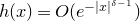
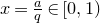
Remark 1.13. The function
 $\sigma(x)$
can be expressed in terms of the Dedekind sum s(x) [Reference Rademacher and GrosswaldRG72]: using [Reference HickersonHic77, Theorem 1], we find
$\sigma(x)$
can be expressed in terms of the Dedekind sum s(x) [Reference Rademacher and GrosswaldRG72]: using [Reference HickersonHic77, Theorem 1], we find
 $$ \sigma(x) = x + \overline x + 12 s(x) \quad (x\in (0, 1)\cap\mathbb{Q}). $$
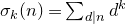
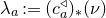
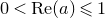
The function
 $\varphi^\triangleright : [0, 1] \to \mathbb{C}$
is depicted in Figure 1. Note that
$\varphi^\triangleright : [0, 1] \to \mathbb{C}$
is depicted in Figure 1. Note that
 $\varphi^\triangleright(0) = 1$
.
$\varphi^\triangleright(0) = 1$
.
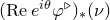
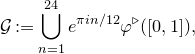
Figure 1. Approximate plots of
 $\operatorname{Re} \varphi^\triangleright$
(a) and
$\operatorname{Re} \varphi^\triangleright$
(a) and
 $\operatorname{Im} \varphi^\triangleright$
(b) defined in (1.12).
$\operatorname{Im} \varphi^\triangleright$
(b) defined in (1.12).
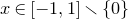
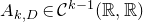
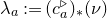
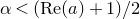
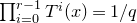
If we normalize
 $\varphi$
by letting
$\varphi$
by letting
 $\varphi^\dagger(x):=\operatorname{Den}(x)^{-3/2}\varphi(x)$
, then as an immediate consequence of Corollary 1.12, we obtain that
$\varphi^\dagger(x):=\operatorname{Den}(x)^{-3/2}\varphi(x)$
, then as an immediate consequence of Corollary 1.12, we obtain that
 $\overline{\varphi^\dagger(\mathbb{Q})}$
is equal to the curve
$\overline{\varphi^\dagger(\mathbb{Q})}$
is equal to the curve
 $\mathcal{G}$
given by
$\mathcal{G}$
given by
 $$ \mathcal{G} := \bigcup_{n=1}^{24} {e}^{\pi i n/12} \varphi^\triangleright([0, 1]), $$
which passes through the 24th roots of unity. In Figure 2a, we have plotted the points
 $\varphi^\triangleright(x)$
for
$\varphi^\triangleright(x)$
for
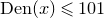 $\operatorname{Den}(x)\leqslant 101$
. The limiting curve is the graph of
$\operatorname{Den}(x)\leqslant 101$
. The limiting curve is the graph of
 $\varphi^\triangleright$
. In Figure 2b, we have plotted the points
$\varphi^\triangleright$
. In Figure 2b, we have plotted the points
 $\varphi^\dagger(x)$
for
$\varphi^\dagger(x)$
for
 $\operatorname{Den}(x)\leqslant 307$
, colored depending on
$\operatorname{Den}(x)\leqslant 307$
, colored depending on
 $\sigma(x)$
. The limiting curve is the curve
$\sigma(x)$
. The limiting curve is the curve
 $\mathcal{G}$
.
$\mathcal{G}$
.

Figure 2. Approximate plots of
 $\varphi^\triangleright([0, 1])$
(a) and
$\varphi^\triangleright([0, 1])$
(a) and
 $\varphi^\dagger([0, 1])$
(b).
$\varphi^\dagger([0, 1])$
(b).
1.3.4 Generalized cotangent sums.
Finally we mention the generalized cotangent functions, studied in [Reference Bettin and ConreyBC13a] and defined for
 $b\in\mathbb{Z}$
,
$b\in\mathbb{Z}$
,
 $q\in\mathbb{N}_{>0}$
, coprime by
$q\in\mathbb{N}_{>0}$
, coprime by
 $$c_a\bigg(\frac bq\bigg):=q^a\sum_{m=1}^{q-1}\cot\bigg(\frac{\pi m b}{q}\bigg)\zeta\bigg(-a,\frac mq\bigg),$$
where
 $a\in \mathbb{C}$
. Here,
$a\in \mathbb{C}$
. Here,
 $\zeta(s,x)$
denotes the Hurwitz zeta function, which is the analytic continuation of
$\zeta(s,x)$
denotes the Hurwitz zeta function, which is the analytic continuation of
 $s\mapsto \sum_{n\geqslant 1} (n+x)^{-s}$
. When
$s\mapsto \sum_{n\geqslant 1} (n+x)^{-s}$
. When
 $a=-1$
, the poles of
$a=-1$
, the poles of
 $\zeta$
cancel out and
$\zeta$
cancel out and
 $c_a$
reduces in that case to the classical Dedekind sum [Reference Rademacher and GrosswaldRG72]. In [Reference Bettin and ConreyBC13a], it was shown that the functions
$c_a$
reduces in that case to the classical Dedekind sum [Reference Rademacher and GrosswaldRG72]. In [Reference Bettin and ConreyBC13a], it was shown that the functions
 $c_a$
are almost quantum modular forms of weight
$c_a$
are almost quantum modular forms of weight
 $1+a$
with period function
$1+a$
with period function
 $h_a$
satisfying, in a neighborhood of 0, the estimate
$h_a$
satisfying, in a neighborhood of 0, the estimate
 $$ h_a(x) = \frac{\zeta(1-a)}{\zeta(-a)}\frac {i}{\pi x} - \textrm{sgn}(x)\cot\bigg(\frac{\pi a}2\bigg)\frac{i}{{| {x} |}^{1+a}} + O(1). $$
The meaning of ‘almost’ here will be made precise later on. The function
 $c_a$
is very closely related to Eichler integrals of certain real-analytic Eisenstein series, see [Reference Bettin and ConreyBC13a, § 2] and [Reference Lewis and ZagierLZ19]. We will deduce from our main results the following statement on the distribution of values of
$c_a$
is very closely related to Eichler integrals of certain real-analytic Eisenstein series, see [Reference Bettin and ConreyBC13a, § 2] and [Reference Lewis and ZagierLZ19]. We will deduce from our main results the following statement on the distribution of values of
 $c_a$
.
$c_a$
.
Corollary 1.14. If
 $\operatorname{Re}(a)<-1$
, then the multiset
$\operatorname{Re}(a)<-1$
, then the multiset
 $$ \{ c_a(b/q) \colon 1\leqslant b \leqslant q, (b, q)=1\} $$
becomes distributed, as
 $q\to \infty$
, according to the measure
$q\to \infty$
, according to the measure
 $\lambda_a := (c_a^\triangleleft)_\ast( \nu)$
. If
$\lambda_a := (c_a^\triangleleft)_\ast( \nu)$
. If
 $\operatorname{Re}(a)>-1$
, then the multiset
$\operatorname{Re}(a)>-1$
, then the multiset
 $$ \{ q^{-1-a} c_a(b/q) \colon 1\leqslant b \leqslant q, (b, q)=1\}$$
becomes distributed, as
 $q\to \infty$
, according to a measure
$q\to \infty$
, according to a measure
 $\lambda_a := (c_a^\triangleright)_\ast( \nu)$
. Moreover:
$\lambda_a := (c_a^\triangleright)_\ast( \nu)$
. Moreover:
-
(1) when
 $a\in (2\mathbb{Z}_{\geqslant0}+1)$
, the measure
$\lambda_a$
is supported on
$\{0\}$
;
$a\in (2\mathbb{Z}_{\geqslant0}+1)$
, the measure
$\lambda_a$
is supported on
$\{0\}$
; -
(2) when
$a\in \mathbb{R}\smallsetminus(2\mathbb{Z}_{\geqslant -1}+1)$
, the measure
$\lambda_a$
is supported inside
$\mathbb{R}$
and is diffuse; -
(3) when
$\operatorname{Re}(a)\neq -1$
and
$a\not\in\mathbb{R}$
, then for any non-zero linear form
$\phi:\mathbb{C}\to\mathbb{R}$
, the push-forward measure
$\phi_\ast(\lambda_a)$
on
$\mathbb{R}$
is diffuse.


When
 $\operatorname{Re}(a)>0$
, the map
$\operatorname{Re}(a)>0$
, the map
 $c_a^\triangleright$
is continuous at irrationals. Moreover, for
$c_a^\triangleright$
is continuous at irrationals. Moreover, for
 $0<\operatorname{Re}(a)\leqslant 1$
, the map
$0<\operatorname{Re}(a)\leqslant 1$
, the map
 $x\mapsto c_a^\triangleright(x)$
is
$x\mapsto c_a^\triangleright(x)$
is
 $\alpha$
-Hölder-continuous locally almost everywhere, for any
$\alpha$
-Hölder-continuous locally almost everywhere, for any
 $\alpha<(\operatorname{Re}(a)+1)/2$
. When
$\alpha<(\operatorname{Re}(a)+1)/2$
. When
 $\operatorname{Re}(a)>1$
, the same is true for the map
$\operatorname{Re}(a)>1$
, the same is true for the map
 $x\mapsto c_a^\triangleright(x) + x a \zeta(1-a)/\pi$
, and in particular the map
$x\mapsto c_a^\triangleright(x) + x a \zeta(1-a)/\pi$
, and in particular the map
 $c_a^\triangleright$
is then differentiable almost everywhere with derivative
$c_a^\triangleright$
is then differentiable almost everywhere with derivative
 $-a\zeta(1-a)/\pi$
.
$-a\zeta(1-a)/\pi$
.
In this statement we have kept the notation
 $c_a^\triangleleft, c_a^\triangleright$
; however, we warn that the actual definitions differ from those in Theorems 1.1 and 1.4, mainly due to the fact
$c_a^\triangleleft, c_a^\triangleright$
; however, we warn that the actual definitions differ from those in Theorems 1.1 and 1.4, mainly due to the fact
 $c_a$
is only ‘almost’ a quantum modular form. The precise definitions are given in § 4.3 below in several cases depending on the value of a.
$c_a$
is only ‘almost’ a quantum modular form. The precise definitions are given in § 4.3 below in several cases depending on the value of a.
In the case (3) above, we obviously also have that
 $\lambda_a$
itself has no atoms.
$\lambda_a$
itself has no atoms.
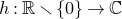
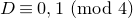
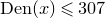
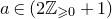
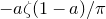
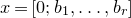
The empirical cumulative distribution functions (CDFs) in Corollary 1.14 for
 $q=5000$
are plotted in Figure 3 for some real values of a. The fact that the corresponding measures are diffuse, stated in item (2) of the previous corollary, translates into the continuity of the limiting functions.
$q=5000$
are plotted in Figure 3 for some real values of a. The fact that the corresponding measures are diffuse, stated in item (2) of the previous corollary, translates into the continuity of the limiting functions.
Figure 3. CDF of the empirical measures at
 $q=5000$
in Corollary 1.14, for
$q=5000$
in Corollary 1.14, for
 $a = -2$
(a) and
$a = -2$
(a) and
 $a = 1/2$
(b).
$a = 1/2$
(b).
The case
 $a=0$
of Corollary 1.14 was studied earlier in [Reference Maier and ThMR16, Reference BettinBet15]. The fact that the values of
$a=0$
of Corollary 1.14 was studied earlier in [Reference Maier and ThMR16, Reference BettinBet15]. The fact that the values of
 $c_0$
have a limiting distribution was proved in [Reference Maier and ThMR16] with an elaborate argument relying on an explicit expression for
$c_0$
have a limiting distribution was proved in [Reference Maier and ThMR16] with an elaborate argument relying on an explicit expression for
 $c_0({\overline b_q}/{q})$
in terms of
$c_0({\overline b_q}/{q})$
in terms of
 $b/q$
(see e.g. [Reference BettinBet15, pp. 1–2]). A simpler proof was then given in [Reference BettinBet15] using an explicit computation of the moments of both the original QMF and the limiting measure. In the generality of Theorem 1.7, and already even in the case
$b/q$
(see e.g. [Reference BettinBet15, pp. 1–2]). A simpler proof was then given in [Reference BettinBet15] using an explicit computation of the moments of both the original QMF and the limiting measure. In the generality of Theorem 1.7, and already even in the case
 $a<-1$
and
$a<-1$
and
 $a\in (-1, 0)$
of Corollary 1.14, the moments don’t exist (see Remark 4.2). The proof of Theorems 1.3 and 1.7 instead identifies directly the limiting function and avoids the computation of moments, thus allowing for more general period functions h.
$a\in (-1, 0)$
of Corollary 1.14, the moments don’t exist (see Remark 4.2). The proof of Theorems 1.3 and 1.7 instead identifies directly the limiting function and avoids the computation of moments, thus allowing for more general period functions h.
It might be interesting to know if the CDF of the Cauchy distribution can be obtained as a limit of the distribution of values of
 $c_a^\triangleright, c_a^\triangleleft$
, appropriately normalized, as
$c_a^\triangleright, c_a^\triangleleft$
, appropriately normalized, as
 $a\to -1$
; in other words, if for some scaling factor
$a\to -1$
; in other words, if for some scaling factor
 $\gamma(a)>0$
, we have
$\gamma(a)>0$
, we have
 $$ \lim_{\substack{a\to -1}} \lambda_a((-\infty, \gamma(a) t]) \overset?= \frac1\pi \int_{-\infty}^t \frac{\mathop{}\!{d} v}{1+v^2} \quad (t\in \mathbb{R}). $$
Indeed, this would match the case
 $a=-1$
(weight zero), for which
$a=-1$
(weight zero), for which
 $c_{-1}(x)$
are the Dedekind sums: it is proved in [Reference VardiVar93] (see [Reference Bettin and DrappeauBD22, § 9.4] for another argument) that the values
$c_{-1}(x)$
are the Dedekind sums: it is proved in [Reference VardiVar93] (see [Reference Bettin and DrappeauBD22, § 9.4] for another argument) that the values
 $c_{-1}(x)$
tend to distribute according to a Cauchy distribution when x is picked at random among rationals of denominators at most Q, as
$c_{-1}(x)$
tend to distribute according to a Cauchy distribution when x is picked at random among rationals of denominators at most Q, as
 $Q\to\infty$
.
$Q\to\infty$
.
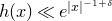
In Figure 4 we present the plots of the real part of
 $c_a^\triangleleft$
and
$c_a^\triangleleft$
and
 $c_a^\triangleright$
for various values of a. The relevant period function
$c_a^\triangleright$
for various values of a. The relevant period function
 $h(x)=h_a(x)$
roughly satisfies
$h(x)=h_a(x)$
roughly satisfies
 $h(x) \sim \kappa(a) x^{-1} + O(1)$
for some constant
$h(x) \sim \kappa(a) x^{-1} + O(1)$
for some constant
 $\kappa(a)$
, see (4.11) later. When
$\kappa(a)$
, see (4.11) later. When
 $\operatorname{Re}(a)<-1$
, we witness a rise in regularity in
$\operatorname{Re}(a)<-1$
, we witness a rise in regularity in
 $c_a^\triangleleft$
as
$c_a^\triangleleft$
as
 $\operatorname{Re}(a)$
decreases, but without reaching full continuity, due to the fact that
$\operatorname{Re}(a)$
decreases, but without reaching full continuity, due to the fact that
 $h_a$
has a pole at 0. When
$h_a$
has a pole at 0. When
 $\operatorname{Re}(a)>0$
, Corollary 1.14 shows that the map
$\operatorname{Re}(a)>0$
, Corollary 1.14 shows that the map
 $c_a^\triangleright$
is continuous at irrationals, and when
$c_a^\triangleright$
is continuous at irrationals, and when
 $\operatorname{Re}(a)>1$
, that it has derivative
$\operatorname{Re}(a)>1$
, that it has derivative
 $-a\zeta(1-a)/\pi$
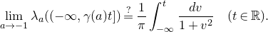
almost everywhere. In Figure 4h, we have
$-a\zeta(1-a)/\pi$
almost everywhere. In Figure 4h, we have
 $a=1.5$
and
$a=1.5$
and
 $-a\zeta(1-a)/\pi \approx 0.09926$
.
$-a\zeta(1-a)/\pi \approx 0.09926$
.
Figure 4. Sample points of
 $c_a$
at N points of denominator q.
$c_a$
at N points of denominator q.
1.4 Notation
1.4.1 General notation.
We set the following general notation:
-
–
$\nu$
is the Lebesgue measure on [0, 1]; -
–
$b_j(x)$
is the jth continued fraction coefficient of x; -
–
$\textrm{Num}(x)$
and
$\operatorname{Den}(x)$
are the numerator and denominator of a rational number x; -
–
$\mu(c_1, \dotsc, c_\ell)$
is the Lebesgue measure of the ‘cylinder set’
$J(c_1, \dotsc, c_\ell)$
defined at (3.10); -
– notation using the letters f, g will typically denote quantum modular forms;
-
– notation using the letter h will denote period functions;
-
– the superscripts
$f^\triangleright$
and
$f^\triangleleft$
refer to continuous extensions defined in (1.3), (1.6), (1.7) or (1.8); -
– T denotes the Gauss map (cf. the next section);
-
– w and
$w_j$
refer to products of iterates of the Gauss map defined in (2.12) and (2.19); -
–
$\vartheta_j$
is a root of unity defined in (2.27); -
– the sets
$\mathfrak{T}(B)$
,
$\mathfrak{S}$
,
$\mathfrak{A}_q$
and
$\mathfrak{T}_q$
are defined in Lemmas 2.2, 3.1 and 3.2; -
– V(B, m, x) and
$\Delta_\lambda(m)$
are defined in (2.6) and (2.7), respectively; -
–
$\mathscr{S}(\lambda)$
is the property defined in Definition 2.4.


Throughout the paper, we use the Vinogradov notation
 $A\ll B$
to mean
$A\ll B$
to mean
 $A = O(B)$
. We denote
$A = O(B)$
. We denote
 $\varpi = {(1 + \sqrt{5})}/{2}$
to be the golden ratio.
$\varpi = {(1 + \sqrt{5})}/{2}$
to be the golden ratio.
1.4.2 The Gauss map, partial quotients, partial denominators.
Let
 $T : \mathbb{R}\smallsetminus\{0\} \to [0, 1)$
,
$T : \mathbb{R}\smallsetminus\{0\} \to [0, 1)$
,
 $T(x):=\{1/x\}$
be the Gauss map,
$T(x):=\{1/x\}$
be the Gauss map,
 $T^i$
its ith iterate. For
$T^i$
its ith iterate. For
 $x\in\mathbb{Q}$
, we let
$x\in\mathbb{Q}$
, we let
 $r:=r(x)$
be the minimum non-negative integer such that
$r:=r(x)$
be the minimum non-negative integer such that
 $T^{r}(x)=0$
and, for
$T^{r}(x)=0$
and, for
 $0\leqslant j < r$
, we write
$0\leqslant j < r$
, we write
 $T^j(x)$
in simplest terms as
$T^j(x)$
in simplest terms as
 \begin{equation} T^j(x) = \frac{u_{j+1}(x)}{u_j(x)}.\end{equation}
In particular, we have
 $$ u_0(x) = \operatorname{Den}(x), \quad u_r(x) = 1 ,$$
where
 $\operatorname{Den}(x)$
is the denominator of x. Whenever
$\operatorname{Den}(x)$
is the denominator of x. Whenever
 $u_{r-1}(x)>1$
, we also define
$u_{r-1}(x)>1$
, we also define
 $$ u_{r+1}(x) := 1, $$
which will be convenient to change the length of the continued fraction (CF) expansion. In the terminology of [Reference Marmi, Moussa and YoccozMMY97], with the value
 $\alpha = 1$
, we have
$\alpha = 1$
, we have
 $u_j(x) = \operatorname{Den}(x) \beta_{j+1}(x)$
. Thus, from [Reference Marmi, Moussa and YoccozMMY97, Proposition 1.4.(iv)] we deduce
$u_j(x) = \operatorname{Den}(x) \beta_{j+1}(x)$
. Thus, from [Reference Marmi, Moussa and YoccozMMY97, Proposition 1.4.(iv)] we deduce
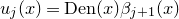
 \begin{equation} \frac{u_j(x)}{u_0(x)} \ll \varpi^{-j}, \quad u_{r-j}(x) \gg \varpi^j \quad\quad \bigg(\varpi=\frac{1+\sqrt{5}}2\bigg). \end{equation}
We will also use the following other decomposition. Given
 $y \in \mathbb{Q}\cap (0, 1)$
and writing uniquely y as its CF expansion
$y \in \mathbb{Q}\cap (0, 1)$
and writing uniquely y as its CF expansion
 $$ y = [0; c_1, \dotsc, c_s] $$
with s odd, we define
 \begin{equation} v_0(y) := 1, \quad v_j(y) := \operatorname{Den}([0; c_1, \dotsc, c_j]) \quad (1\leqslant j \leqslant s).\end{equation}
Equivalently,
 $v_j(y) = \operatorname{Den}([0; c_j, \dotsc, c_1])$
. Note that, with
$v_j(y) = \operatorname{Den}([0; c_j, \dotsc, c_1])$
. Note that, with
 $\overline{y} = [0; c_s, \dotsc, c_1]$
, we have
$\overline{y} = [0; c_s, \dotsc, c_1]$
, we have
 $$ v_j(y) = u_{s-j}(\overline{y}), $$
and as such
 \begin{equation} v_j(y) \gg \varpi^j. \end{equation}
We refer to Khinchin’s book [Reference KhintchineKhi63] and to the survey [Reference Flajolet, Vallée and VardiFVV] for additional information about continued fractions.
2. Extending the domain of quantum modular forms
In this section we prove Theorems 1.1, 1.2, 1.4 and 1.5.
2.1 Iteration of the reciprocity formula
First, we notice that by Euclid’s algorithm, any QMF f of level 1 is determined by h and its value at 0. Indeed, by repeatedly applying (1.2) and periodicity, we obtain, for
 $x=\frac aq\in[0,1)$
in reduced form,
$x=\frac aq\in[0,1)$
in reduced form,
 \begin{equation} f(x)=\sum_{j=0}^{r-1}\bigg(\prod_{i=0}^{j-1}T^{i}(x)\bigg)^{\!{-}k} h((-1)^{j}T^j(x))+q^{k} f(0).\end{equation}
Notice that we used that
 $\prod_{i=0}^{r-1}T^{i}(x)=1/q$
.
$\prod_{i=0}^{r-1}T^{i}(x)=1/q$
.
The above quantities are naturally expressed in terms of continued fractions. Indeed, if
 $x\in(0,1)$
, then the length of its CF expansion
$x\in(0,1)$
, then the length of its CF expansion
 $x=[0;b_1,\ldots,b_{r}]$
with minimal length (i.e.
$x=[0;b_1,\ldots,b_{r}]$
with minimal length (i.e.
 $b_{r}\neq1$
if
$b_{r}\neq1$
if
 $r>1$
) is r. Also, for
$r>1$
) is r. Also, for
 $0\leqslant j\leqslant r$
we have
$0\leqslant j\leqslant r$
we have
 $q \prod_{i=0}^{j-1}T^{i}(x)=(\prod_{i=j}^{r-1}T^{i}(x))^{-1}$
is the denominator
$q \prod_{i=0}^{j-1}T^{i}(x)=(\prod_{i=j}^{r-1}T^{i}(x))^{-1}$
is the denominator
 $u_{j}(x)$
defined in (1.15). Notice also that
$u_{j}(x)$
defined in (1.15). Notice also that
 $u_0(x)=q$
. Thus, abbreviating
$u_0(x)=q$
. Thus, abbreviating
 $u_j = u_j(x)$
, we can then rewrite (2.1) as
$u_j = u_j(x)$
, we can then rewrite (2.1) as
 \begin{equation} f(x)=\sum_{j=0}^{r-1}\bigg(\frac{u_j}{u_0}\bigg)^{\!{-}k} h\bigg((-1)^{j}\frac{u_{j+1}}{u_{j}}\bigg) + u_0^{k} f(0).\end{equation}
This formula holds also if r is formally replaced by
 $r+1$
, which corresponds to expressing
$r+1$
, which corresponds to expressing
 $x = [0;b_1,\ldots,b_{r}]$
rather as
$x = [0;b_1,\ldots,b_{r}]$
rather as
 $[0; b_1, \dotsc, b_r - 1, 1]$
, since the additional term in (2.2) is
$[0; b_1, \dotsc, b_r - 1, 1]$
, since the additional term in (2.2) is
 \begin{equation} u_0^k h((-1)^r) = u_0^k(f(0)-f(0)) = 0,\end{equation}
by (1.2) and periodicity.
Finally, we deduce another variant of (2.2). First, we notice that if
 $[0;b_1,\ldots,b_r]$
is the CF expansion of
$[0;b_1,\ldots,b_r]$
is the CF expansion of
 $x\neq0$
with r odd, then
$x\neq0$
with r odd, then
 $\overline x=[0;b_r,\ldots,b_1]$
. In particular, after the change of variables
$\overline x=[0;b_r,\ldots,b_1]$
. In particular, after the change of variables
 $r\to r-j$
, (2.2) can be rewritten as
$r\to r-j$
, (2.2) can be rewritten as
 \begin{equation} q^{-k}f(x)=\Psi(\overline x)\end{equation}
where, for
 $y=[0;c_1,\ldots,c_r]$
with r odd, and the notation (1.17),
$y=[0;c_1,\ldots,c_r]$
with r odd, and the notation (1.17),
 \begin{equation} \Psi(y):=\sum_{j=1}^{r}v_{j}^{-k}h\bigg((-1)^{j-1}\frac{v_{j-1}}{v_{j}}\bigg)+f(0).\end{equation}
From the expansions (2.2) and (2.5), and the fact that both quantities
 $u_j/u_0$
and
$u_j/u_0$
and
 $v_j^{-1}$
decrease exponentially fast with j, we see the difference of behavior according to the sign of
$v_j^{-1}$
decrease exponentially fast with j, we see the difference of behavior according to the sign of
 $\operatorname{Re}(k)$
, and the relevance of switching x to
$\operatorname{Re}(k)$
, and the relevance of switching x to
 $\overline x$
when
$\overline x$
when
 $\operatorname{Re}(k)>0$
.
$\operatorname{Re}(k)>0$
.
Finally, we need the following simple fact.
Lemma 2.1. Let
 $x\in\mathbb{Q}$
. Then, there exists a neighborhood
$x\in\mathbb{Q}$
. Then, there exists a neighborhood
 $I_x$
of x such that
$I_x$
of x such that
 $r(y)\geqslant r(x)+1$
for all
$r(y)\geqslant r(x)+1$
for all
 $y\in I_x\smallsetminus\{x\}$
.
$y\in I_x\smallsetminus\{x\}$
.
Proof. The statement is immediate if
 $x\in\mathbb{Z}$
. Now let
$x\in\mathbb{Z}$
. Now let
 $x=[b_0;b_1,\ldots,b_r]\in\mathbb{Q}\smallsetminus \mathbb{Z}$
with
$x=[b_0;b_1,\ldots,b_r]\in\mathbb{Q}\smallsetminus \mathbb{Z}$
with
 $r:=r(x)$
. In particular,
$r:=r(x)$
. In particular,
 $b_r>1$
. Assume r is odd. Then the statement holds for
$b_r>1$
. Assume r is odd. Then the statement holds for
 $I_x=(L_x,R_x)$
, where
$I_x=(L_x,R_x)$
, where
 $L_x=[0;b_1,\ldots,b_r+1]$
,
$L_x=[0;b_1,\ldots,b_r+1]$
,
 $R_x=[0;b_1,\ldots,b_r-1]$
. Indeed, if
$R_x=[0;b_1,\ldots,b_r-1]$
. Indeed, if
 $y\in(L_x,x)$
then
$y\in(L_x,x)$
then
 $y=[0;b_1,\ldots,b_r,\alpha]$
for some
$y=[0;b_1,\ldots,b_r,\alpha]$
for some
 $\alpha\in\mathbb{R}_{>1}$
, whereas if
$\alpha\in\mathbb{R}_{>1}$
, whereas if
 $y\in(x,R_x)$
then
$y\in(x,R_x)$
then
 $y=[0;b_1,\ldots,b_r-1,\alpha]$
for some
$y=[0;b_1,\ldots,b_r-1,\alpha]$
for some
 $\alpha\in\mathbb{R}_{>1}$
. In either case
$\alpha\in\mathbb{R}_{>1}$
. In either case
 $T^{r}(y)=1/\alpha \neq0$
and thus
$T^{r}(y)=1/\alpha \neq0$
and thus
 $r(y)>r$
. The case of r even is identical with the role of
$r(y)>r$
. The case of r even is identical with the role of
 $L_x$
and
$L_x$
and
 $R_x$
reversed.
$R_x$
reversed.
2.2 Continuity almost everywhere and extension
In this section, we state and prove a technical proposition which will be helpful when extending f almost everywhere in Theorems 1.2 and 1.5.
We first need the following lemma, which follows readily from a result of Khinchin [Reference KhintchineKhi63, Theorem 30]. In the following we will use the notation
 $r(x)=\infty$
if
$r(x)=\infty$
if
 $x\notin\mathbb{Q}$
.
$x\notin\mathbb{Q}$
.
Lemma 2.2. For each
 $B>0$
, let
$B>0$
, let
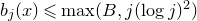
 $$ \mathfrak{T}(B) := \{x\in\mathbb{R} \colon b_j(x) \leqslant \max(B, j(\log j)^2)\text{ for all } 1\leqslant j\leqslant r(x)\}. $$
The set
 $\mathfrak{T}(B)$
is invariant under
$\mathfrak{T}(B)$
is invariant under
 $x\mapsto x+1$
. Moreover,
$x\mapsto x+1$
. Moreover,
 $\nu(\mathfrak{T}(B)\cap[0, 1]) = 1 + o(1)$
as
$\nu(\mathfrak{T}(B)\cap[0, 1]) = 1 + o(1)$
as
 $B\to\infty$
and the set
$B\to\infty$
and the set
 $$ \mathfrak{S} = \bigcup_{B>0} \mathfrak{T}(B) $$
is of full Lebesgue measure.
Proof. By [Reference KhintchineKhi63, Theorem 30] one deduces that
 $\mathfrak{S}$
has full measure. Since
$\mathfrak{S}$
has full measure. Since
 $ \mathfrak{T}(B')\subseteq \mathfrak{T}(B)$
if
$ \mathfrak{T}(B')\subseteq \mathfrak{T}(B)$
if
 $0<B'\leqslant B$
, one then deduces that
$0<B'\leqslant B$
, one then deduces that
 $\nu(\mathfrak{T}(B)\cap[0, 1]) = 1 + o(1)$
as
$\nu(\mathfrak{T}(B)\cap[0, 1]) = 1 + o(1)$
as
 $B\to\infty$
. Finally, the invariance under
$B\to\infty$
. Finally, the invariance under
 $x\mapsto x+1$
is clear since the conditions in
$x\mapsto x+1$
is clear since the conditions in
 $\mathfrak{T}(B)$
don’t involve
$\mathfrak{T}(B)$
don’t involve
 $b_0$
.
$b_0$
.
Remark 2.3. Lemma 2.2 holds with the condition
 $b_j(x) \leqslant \max(B, j(\log j)^2)$
replaced by
$b_j(x) \leqslant \max(B, j(\log j)^2)$
replaced by
 $b_j(x) \leqslant \max(B,a_j)$
for any non-negative increasing sequence
$b_j(x) \leqslant \max(B,a_j)$
for any non-negative increasing sequence
 $(a_j)_j$
such that
$(a_j)_j$
such that
 $\sum_{j\geqslant 1}a_j^{-1}$
converges. For our later purposes we will also need that
$\sum_{j\geqslant 1}a_j^{-1}$
converges. For our later purposes we will also need that
 $a_j\ll_\varepsilon j^{1+\varepsilon}$
for all
$a_j\ll_\varepsilon j^{1+\varepsilon}$
for all
 $\varepsilon>0$
. Making the explicit choice
$\varepsilon>0$
. Making the explicit choice
 $a_j=j(\log j)^2$
simplifies the notation in later computations.
$a_j=j(\log j)^2$
simplifies the notation in later computations.
Given
 $B>0$
, an integer
$B>0$
, an integer
 $m\geqslant 1$
and a number
$m\geqslant 1$
and a number
 $x\in \mathfrak{T}(B)$
, define
$x\in \mathfrak{T}(B)$
, define
 \begin{equation} V(B, m, x) := \{ x' \in \mathbb{Q}\cap \mathfrak{T}(B) \colon r(x') \geqslant m,\ \forall j\leqslant m, b_j(x') = b_j(x) \},\end{equation}
the set of all rationals in
 $\mathfrak{T}(B)$
whose first m coefficients coincide with those of x.
$\mathfrak{T}(B)$
whose first m coefficients coincide with those of x.
Definition 2.4 (Property
 $\mathscr{S}(\lambda)$
.) We say that
$\mathscr{S}(\lambda)$
.) We say that
 $f:\mathbb{Q}\to\mathbb{C}$
has the property
$f:\mathbb{Q}\to\mathbb{C}$
has the property
 $\mathscr{S}(\lambda)$
if the quantity
$\mathscr{S}(\lambda)$
if the quantity
 \begin{equation} \Delta_\lambda(m) := \sup_{x\in\mathfrak{T}(m^\lambda)} \sup_{x', x'' \in V(m^\lambda, m, x)} {| {f(x') - f(x'')} |} \end{equation}
satisfies
 \begin{equation} \Delta_\lambda(m) \to 0 \end{equation}
as
 $m\to\infty$
.
$m\to\infty$
.
Proposition 2.5. Let
 $\lambda>1$
, and assume that f has the property
$\lambda>1$
, and assume that f has the property
 $\mathscr{S}(\lambda)$
. Then for any
$\mathscr{S}(\lambda)$
. Then for any
 $x\in \mathfrak{S} \smallsetminus\mathbb{Q}$
, the limit
$x\in \mathfrak{S} \smallsetminus\mathbb{Q}$
, the limit
 \begin{equation} f^*(x) := \lim_{y\in \mathbb{Q}\cap\mathfrak{T}(B), y\to x} f(y)\end{equation}
exists for any
 $B>0$
such that
$B>0$
such that
 $x\in \mathfrak{T}(B)\smallsetminus\mathbb{Q}$
. Moreover, let
$x\in \mathfrak{T}(B)\smallsetminus\mathbb{Q}$
. Moreover, let
 $m\in\mathbb{N}$
and
$m\in\mathbb{N}$
and
 $B>0$
be given with
$B>0$
be given with
 $m \geqslant B^{1/\lambda}$
, and define
$m \geqslant B^{1/\lambda}$
, and define
 $f^*(x) := f(x)$
for
$f^*(x) := f(x)$
for
 $x\in\mathbb{Q}$
. Then uniformly in
$x\in\mathbb{Q}$
. Then uniformly in
 $x, x' \in \mathfrak{T}(B)$
satisfying
$x, x' \in \mathfrak{T}(B)$
satisfying
 $r(x), r(x')\geqslant m$
and
$r(x), r(x')\geqslant m$
and
 $b_j(x) = b_j(x')$
for
$b_j(x) = b_j(x')$
for
 $j\leqslant m$
, we have
$j\leqslant m$
, we have
 \begin{equation} f^*(x) - f^*(x') = o(1) \quad (m\to \infty), \end{equation}
where the rate of decay may depend on
 $\lambda$
, but not on B.
$\lambda$
, but not on B.
Remark 2.6. Let
 $x\in \mathfrak{T}(B)\smallsetminus\mathbb{Q}$
. Since
$x\in \mathfrak{T}(B)\smallsetminus\mathbb{Q}$
. Since
 $\mathfrak{T}(B') \subset \mathfrak{T}(B)$
for
$\mathfrak{T}(B') \subset \mathfrak{T}(B)$
for
 $B \geqslant B' > 0$
, from (2.9) we also get
$B \geqslant B' > 0$
, from (2.9) we also get
 $f^*(x) = \lim_{y\in\mathbb{Q}\cap \mathfrak{T}(B'), y\to x} f(y)$
, for any
$f^*(x) = \lim_{y\in\mathbb{Q}\cap \mathfrak{T}(B'), y\to x} f(y)$
, for any
 $0<B'<B$
with
$0<B'<B$
with
 $x\in \mathfrak{T}(B')\smallsetminus\mathbb{Q}$
. In particular, the existence of the limit implies that its value
$x\in \mathfrak{T}(B')\smallsetminus\mathbb{Q}$
. In particular, the existence of the limit implies that its value
 $f^*(x)$
is independent of B. Notice that the rate of convergence, however, might depend on it.
$f^*(x)$
is independent of B. Notice that the rate of convergence, however, might depend on it.
Proof of Proposition 2.5. Let
 $x\in \mathfrak{T}(B)\smallsetminus\mathbb{Q}$
. We wish to show that the limit (2.9) exists. By Cauchy’s criterion, it suffices to show that
$x\in \mathfrak{T}(B)\smallsetminus\mathbb{Q}$
. We wish to show that the limit (2.9) exists. By Cauchy’s criterion, it suffices to show that
 \begin{align} \lim_{\varepsilon\to 0^+} \sup_{\substack{x', x'' \in \mathbb{Q} \cap\mathfrak{T}(B) \\ {| {x'-x} |}, {| {x''-x} |} \leqslant \varepsilon}} {| {f(x') - f(x'')} |} = 0. \end{align}
Let
 $\varepsilon>0$
. Since
$\varepsilon>0$
. Since
 $x\not\in\mathbb{Q}$
, we may find
$x\not\in\mathbb{Q}$
, we may find
 $m\in\mathbb{N}$
such that for any
$m\in\mathbb{N}$
such that for any
 $y\in\mathbb{Q}\cap[x-\varepsilon, x+\varepsilon]$
, then
$y\in\mathbb{Q}\cap[x-\varepsilon, x+\varepsilon]$
, then
 $r(y)>m$
and
$r(y)>m$
and
 $b_j(y) = b_j(x)$
for all
$b_j(y) = b_j(x)$
for all
 $j\leqslant m$
. Clearly,
$j\leqslant m$
. Clearly,
 $m\to\infty$
as
$m\to\infty$
as
 $\varepsilon\to0^+.$
In particular, we can assume
$\varepsilon\to0^+.$
In particular, we can assume
 $m\geqslant B^{1/\lambda}$
so that
$m\geqslant B^{1/\lambda}$
so that
 $\mathfrak{T}(B) \subset \mathfrak{T}(m^\lambda)$
. Thus,
$\mathfrak{T}(B) \subset \mathfrak{T}(m^\lambda)$
. Thus,
 $x\in\mathfrak{T}(m^\lambda)$
and
$x\in\mathfrak{T}(m^\lambda)$
and
 $\mathbb{Q}\cap[x-\varepsilon, x+\varepsilon]\cap \mathfrak{T}(B)\subseteq V(m^\lambda,m,x)$
and (2.11) follows from (2.8).
$\mathbb{Q}\cap[x-\varepsilon, x+\varepsilon]\cap \mathfrak{T}(B)\subseteq V(m^\lambda,m,x)$
and (2.11) follows from (2.8).
It remains to show (2.10). Let
 $x, x' \in \mathfrak{T}(B)$
,
$x, x' \in \mathfrak{T}(B)$
,
 $m \geqslant B^{1/\lambda}$
, and for
$m \geqslant B^{1/\lambda}$
, and for
 $0\leqslant j \leqslant m$
, define
$0\leqslant j \leqslant m$
, define
 $b_j := b_j(x) = b_j(x')$
. Consider the convergents
$b_j := b_j(x) = b_j(x')$
. Consider the convergents
 $(x_\ell)$
,
$(x_\ell)$
,
 $(x'_\ell)$
of x and x’, respectively, so that, for instance,
$(x'_\ell)$
of x and x’, respectively, so that, for instance,
 $$ x_\ell = [b_0; b_1, \dotsc, b_m, b_{m+1}(x), \dotsc, b_{\ell}(x)] \quad (m\leqslant \ell \leqslant r(x)). $$
Also, consider the rational
 $y := [b_0; b_1, \ldots, b_m]$
. We have
$y := [b_0; b_1, \ldots, b_m]$
. We have
 $y\in\mathfrak{T}(m^{\lambda})$
by hypothesis on m. We obviously also have
$y\in\mathfrak{T}(m^{\lambda})$
by hypothesis on m. We obviously also have
 $x_\ell\in V(m,m^{\lambda},y)$
whenever
$x_\ell\in V(m,m^{\lambda},y)$
whenever
 $m\leqslant \ell \leqslant r(x)$
, and similarly
$m\leqslant \ell \leqslant r(x)$
, and similarly
 $x'_\ell \in V(m,m^{\lambda},y)$
for
$x'_\ell \in V(m,m^{\lambda},y)$
for
 $m\leqslant \ell \leqslant r(x')$
. We deduce that
$m\leqslant \ell \leqslant r(x')$
. We deduce that
 ${| {f(x_\ell) - f(x'_{\ell'})} |} \leqslant \Delta_{\lambda}(m)$
with the notation (2.8), and therefore
${| {f(x_\ell) - f(x'_{\ell'})} |} \leqslant \Delta_{\lambda}(m)$
with the notation (2.8), and therefore
 $$ {| {f^*(x) - f^*(x')} |} \leqslant \Delta_{\lambda}(m) $$
by taking
 $\ell = r(x)$
if
$\ell = r(x)$
if
 $x\in\mathbb{Q}$
or
$x\in\mathbb{Q}$
or
 $\ell\to\infty$
if
$\ell\to\infty$
if
 $x\not\in\mathbb{Q}$
, and similarly for x’. The right-hand side does not depend on B and tends to 0 by (2.8), which is what we claimed.
$x\not\in\mathbb{Q}$
, and similarly for x’. The right-hand side does not depend on B and tends to 0 by (2.8), which is what we claimed.
2.3 The case of
$\operatorname{Re}(k)<0$

In this section we prove Theorems 1.1 and 1.2. We start by a lemma regarding the size and regularity of products of consecutive iterates of the Gauss map.
Lemma 2.7. Let
 $j\in\mathbb{N}$
,
$j\in\mathbb{N}$
,
 $\tau\in\mathbb{C}$
and
$\tau\in\mathbb{C}$
and
 $g:[0, 1] \to \mathbb{C}$
. For
$g:[0, 1] \to \mathbb{C}$
. For
 $x\in [0, 1)$
, define
$x\in [0, 1)$
, define
 \begin{equation} w(x) = w(x; j, \tau, g) := \mathbf{1}(j\leqslant r(x)) \bigg(\prod_{i=0}^{j-1} T^i(x)\bigg)^{\!\tau} g(T^j(x)), \end{equation}
where we recall that
 $r(x) = +\infty$
by convention if
$r(x) = +\infty$
by convention if
 $x\not\in\mathbb{Q}$
and
$x\not\in\mathbb{Q}$
and
 $\mathbf{1}(j\leqslant r(x))$
indicates the indicator function of the condition
$\mathbf{1}(j\leqslant r(x))$
indicates the indicator function of the condition
 $j\leqslant r(x)$
.
$j\leqslant r(x)$
.
-
– If
$\operatorname{Re}(\tau)>0$
and g is continuous, then w is continuous on
$[0, 1)\smallsetminus \{x, r(x)\in\{j-1,j\} \}$
. Moreover, letting
$\pm 1 = (-1)^j$
, we have (2.13)
\begin{align} & w(x^\pm) = \operatorname{Den}(x)^{-\tau} g(0) && (r(x) \in \{j-1, j\}), \notag\\ & w(x^\mp) = \operatorname{Den}(x)^{-\tau} g(1) && (r(x) = j), \\ & w(x^\mp) = 0 && (r(x)=j-1).\notag \end{align}
-
– If
$\operatorname{Re}(\tau)>2$
and g is of
$\mathcal{C}^1$
class, then w is of
$\mathcal{C}^1$
class on
$[0, 1)\smallsetminus \{x, r(x)\in\{j-1,j\} \}$
. When
$r(x)\not\in\{j-1, j\}$
, we have (2.14)Moreover, we have
\begin{align} w'(x) = \mathbf{1}(j\leqslant r(x)) \bigg\{& \tau g(T^j(x)) \sum_{i=0}^{j-1} (-1)^i \bigg(\prod_{0\leqslant \ell < i} T^\ell(x)\bigg)^{\!\tau-2} T^i(x)^{\tau-1} \bigg(\prod_{i<\ell<j} T^\ell(x)\bigg)^{\!\tau} \nonumber\\ {}& + (-1)^j g'(T^j(x)) \bigg(\prod_{0\leqslant \ell < j} T^\ell(x)\bigg)^{\!\tau-2}\bigg\}. \end{align}
(2.15)
\begin{align} & w'(x^\pm) = \operatorname{Den}(x)^{-\tau+2}\bigg(\tau g(0)\sum_{i=0}^{j-1}\frac{(-1)^i}{u_i(x)u_{i+1}(x)} \pm g'(0)\bigg) && (r(x) \in \{j-1, j\}), \notag\\ & w'(x^\mp) = \operatorname{Den}(x)^{-\tau+2} \bigg(\tau g(1)\sum_{i=0}^{j-1}\frac{(-1)^i}{u_i(x)u_{i+1}(x)} \pm g'(1)\bigg) && (r(x) = j), \\ & w'(x^\mp) = 0 && (r(x) = j-1).\notag \end{align}
-
– If
$\operatorname{Re}(\tau)>0$
and
$g\in\mathcal{C}^0$
, we have (2.16)while if
\begin{equation} \|w\|_\infty \leqslant \varpi^{\operatorname{Re}(\tau)(1 - j)} \|g\|_\infty, \end{equation}
$\operatorname{Re}(\tau)>2$
and
$g\in\mathcal{C}^1$
, we have (2.17)
\begin{equation} \|w'\|_\infty \leqslant j {| {\tau} |} \varpi^{(\operatorname{Re}(\tau)-2)(1-j)}(\|g\|_\infty + \|g'\|_\infty). \end{equation}


Remark 2.8. The bound (2.16) is essentially contained in the paper [Reference Marmi, Moussa and YoccozMMY97, Theorem 2.6]. This paper contains also results pertaining to
 $L^p$
, Hölder and BMO regularity of products of the shape w(x). The proof of Lemma 2.7 and the arguments in [Reference Marmi, Moussa and YoccozMMY97] both make use of the iterative structure of w(x) (compare (2.18) below and [Reference Marmi, Moussa and YoccozMMY97, Equation (2.13)]), with the computation of the one-sided limits at rationals (2.13) and (2.15) requiring additional care.
$L^p$
, Hölder and BMO regularity of products of the shape w(x). The proof of Lemma 2.7 and the arguments in [Reference Marmi, Moussa and YoccozMMY97] both make use of the iterative structure of w(x) (compare (2.18) below and [Reference Marmi, Moussa and YoccozMMY97, Equation (2.13)]), with the computation of the one-sided limits at rationals (2.13) and (2.15) requiring additional care.
Proof.
Value of w’. For the convenience of our argument, we start by noting that if
 $g\in \mathcal{C}^1$
and
$g\in \mathcal{C}^1$
and
 $\operatorname{Re}(\tau)>2$
, then whenever
$\operatorname{Re}(\tau)>2$
, then whenever
 $r(x)>j$
, the right-hand side of (2.12) defines a
$r(x)>j$
, the right-hand side of (2.12) defines a
 $\mathcal{C}^1$
function in a neighborhood of x. When
$\mathcal{C}^1$
function in a neighborhood of x. When
 $m\geqslant1$
, its derivative can be computed using the expression
$m\geqslant1$
, its derivative can be computed using the expression
 \begin{align*} (T^i)'(x) = (-1)^i \bigg(\prod_{0\leqslant \ell < i}T^\ell(x)\bigg)^{\!{-}2}, \end{align*}
and this leads to the given formula for w’(x).
Regularity. We treat the continuity and differentiability claims simultaneously, proving the following more general assertion: given
 $m\in\{0, 1\}$
,
$m\in\{0, 1\}$
,
 $j\geqslant 1$
and
$j\geqslant 1$
and
 $\operatorname{Re}(\tau)>2m$
, if there is a countable set S for which g is
$\operatorname{Re}(\tau)>2m$
, if there is a countable set S for which g is
 $\mathcal{C}^m$
on
$\mathcal{C}^m$
on
 $[0, 1]\smallsetminus S$
, then
$[0, 1]\smallsetminus S$
, then
 $x\mapsto w(j, \tau, g)$
is
$x\mapsto w(j, \tau, g)$
is
 $\mathcal{C}^m$
on the set
$\mathcal{C}^m$
on the set
 $$ [0, 1] \smallsetminus \{x: r(x)\in\{j-1, j\} \text{ or } (r(x)>j \text{ and } T^j(x) \in S)\}. $$
We proceed by induction. Assume first
 $j=1$
. We have
$j=1$
. We have
 $r(x)\geqslant 1 \iff x\neq 0$
, so that
$r(x)\geqslant 1 \iff x\neq 0$
, so that
 $$ w(x; 1, \tau, g) = \mathbf{1}(x\neq 0) x^\tau g(T(x)). $$
This function is easily seen to be
 $\mathcal{C}^m$
at
$\mathcal{C}^m$
at
 $x\in[0, 1]$
whenever
$x\in[0, 1]$
whenever
 $x>0$
,
$x>0$
,
 $T(x) \in (0, 1)$
and
$T(x) \in (0, 1)$
and
 $T(x) \not \in S$
. These conditions amount to
$T(x) \not \in S$
. These conditions amount to
 $r(x) > 1$
and
$r(x) > 1$
and
 $T(x) \not\in S$
, which gives our claim in the case
$T(x) \not\in S$
, which gives our claim in the case
 $j=1$
.
$j=1$
.
Let
 $j>1$
, and suppose our claim is proven for
$j>1$
, and suppose our claim is proven for
 $j-1$
. Then we note that
$j-1$
. Then we note that
 \begin{equation} w(x; j, \tau, g) = w(x; 1, \tau, [x\mapsto w(x; j-1, \tau, g)]). \end{equation}
By induction, the function
 $x\mapsto w(x; j-1, \tau, g)$
is
$x\mapsto w(x; j-1, \tau, g)$
is
 $\mathcal{C}^m$
on
$\mathcal{C}^m$
on
 $[0, 1]\smallsetminus S'$
, where
$[0, 1]\smallsetminus S'$
, where
 $$ S' = \{x, r(x) \in \{j-2, j-1\}\text{ or } (r(x)>j-1 \text{ and } T^{j-1}(x) \in S)\}. $$
The set S’ is again countable, since
 $T^{j-1}$
has countably many inverse branches. From the case
$T^{j-1}$
has countably many inverse branches. From the case
 $j=1$
of our claim, we deduce that
$j=1$
of our claim, we deduce that
 $x\mapsto w(x; j, \tau, g)$
is
$x\mapsto w(x; j, \tau, g)$
is
 $\mathcal{C}^m$
on
$\mathcal{C}^m$
on
 $[0, 1]\smallsetminus S''$
, where
$[0, 1]\smallsetminus S''$
, where
 \begin{align*} S'' ={}& \{x, r(x) \in \{0, 1\} \text{ or } (r(x)>1\text{ and } T(x) \in S'\} \\ = {}& \{x, r(x) \in \{0, 1, j-1, j\} \text{ or } (r(x)>j\text{ and } T^j(x) \in S)\} \end{align*}
by definition of S’. It remains to check that w is
 $\mathcal{C}^m$
at x if
$\mathcal{C}^m$
at x if
 $r(x) = 0$
and
$r(x) = 0$
and
 $j\geqslant 2$
, or if
$j\geqslant 2$
, or if
 $r(x) = 1$
and
$r(x) = 1$
and
 $j\geqslant 3$
. But supposing
$j\geqslant 3$
. But supposing
 $r(x) = 1$
, we have for
$r(x) = 1$
, we have for
 $\varepsilon\to 0^+$
,
$\varepsilon\to 0^+$
,
 $$ T(x-\varepsilon) = O(\varepsilon), \quad T(x+\varepsilon) = 1-O(\varepsilon)\ \Rightarrow\ T^2(x+\varepsilon) = O(\varepsilon), $$
and therefore, we have in any case
 $\lim_{y\to x} T(y) T^2(y) = O({| {x-y} |})$
. Thus, if
$\lim_{y\to x} T(y) T^2(y) = O({| {x-y} |})$
. Thus, if
 $j\geqslant 3$
and
$j\geqslant 3$
and
 $\operatorname{Re}(\tau)>2m$
, we then have as
$\operatorname{Re}(\tau)>2m$
, we then have as
 $y\to x$
,
$y\to x$
,
 $$ w(y; j, \tau, g) = O((T(y) T^2(y))^{\operatorname{Re}(\tau)}) = o({| {x-y} |}^m), $$
and so w is continuous at x, and differentiable there when
 $m=1$
, with derivative 0. Moreover, if
$m=1$
, with derivative 0. Moreover, if
 $m=1$
, by the explicit expression (2.14) and the bounds above, we find
$m=1$
, by the explicit expression (2.14) and the bounds above, we find
 $$ w'(y) = O({| {x-y} |}^{\operatorname{Re}(\tau)-2}) = o(1), $$
and therefore w is
 $\mathcal{C}^m$
at x. A similar argument holds when
$\mathcal{C}^m$
at x. A similar argument holds when
 $r(x) = 0$
, and concludes the proof of our claim.
$r(x) = 0$
, and concludes the proof of our claim.
Limits of w. Assume
 $r(x) = j$
. Note that for
$r(x) = j$
. Note that for
 $y\neq x$
in the neighborhood of x, we have
$y\neq x$
in the neighborhood of x, we have
 $r(y)>r(x)$
, and moreover
$r(y)>r(x)$
, and moreover
 $$ \lim_{y\to x^\pm} T^j(y) = 0, \quad \lim_{y\to x^\mp} T^j(y) = 1. $$
The expression given for
 $w(x^\pm)$
and
$w(x^\pm)$
and
 $w(x^\mp)$
then follows upon taking the limit in the expression (2.12). The case when
$w(x^\mp)$
then follows upon taking the limit in the expression (2.12). The case when
 $r(x)=j-1$
is similar, using instead the limits
$r(x)=j-1$
is similar, using instead the limits
 $$ \lim_{y\to x^\pm} T^j(y) = \lim_{y\to x^\mp} T^{j-1}(y) = 0. $$
Limits of w’. The expressions given for
 $w'(x^\pm)$
when
$w'(x^\pm)$
when
 $r(x) \in\{j-1, j\}$
follow from an argument identical to the computation of the limits
$r(x) \in\{j-1, j\}$
follow from an argument identical to the computation of the limits
 $w(x^\pm)$
. In the claimed formulae, we have used the notation (1.15) (for x rational).
$w(x^\pm)$
. In the claimed formulae, we have used the notation (1.15) (for x rational).
Bounds. The bounds (2.16), (2.17) follow immediately from the explicit expressions above, along with the argument of [Reference Marmi, Moussa and YoccozMMY97, Proposition 1.4.(iv)].
2.3.1 Proof of Theorem 1.1. The domain of
$f^\triangleleft$
.

In this section we show that
 $f^\triangleleft(x)$
is defined for all
$f^\triangleleft(x)$
is defined for all
 $x\in\mathbb{R}$
. By periodicity, we can assume
$x\in\mathbb{R}$
. By periodicity, we can assume
 $x\in (0,1)\smallsetminus\mathbb{Q}$
. We also recall that h is bounded on
$x\in (0,1)\smallsetminus\mathbb{Q}$
. We also recall that h is bounded on
 $[-1,1]$
by hypothesis. We let
$[-1,1]$
by hypothesis. We let
 \begin{align} h_j(y) := h((-1)^j y), \quad w_j(y) := w(y, j, -k, h_j),\end{align}
for
 $y>0$
, and extend
$y>0$
, and extend
 $h_j$
at
$h_j$
at
 $y=0$
by continuity, so that in particular
$y=0$
by continuity, so that in particular
 \begin{equation} w_{r(x')}(x')=\operatorname{Den}(x') ^k h(0^\pm)\quad (x'\in\mathbb{Q},\ \pm = (-1)^{r(x')}).\end{equation}
Thus, with this notation, (2.1) reads
 \begin{equation} f(x') = \sum_{j\geqslant 0} w_j(x') + \operatorname{Den}(x') ^k(f(0)-h(0^\pm)). \end{equation}
It suffices to show that
 $\sup |f(x')-f(x'')|\to0$
as
$\sup |f(x')-f(x'')|\to0$
as
 $\varepsilon\to0$
, where the sup is over all
$\varepsilon\to0$
, where the sup is over all
 $x',x''\in\mathbb{Q}$
with
$x',x''\in\mathbb{Q}$
with
 $|x-x'|,|x-x''|<\varepsilon$
. Since
$|x-x'|,|x-x''|<\varepsilon$
. Since
 $x\not\in\mathbb{Q}$
, there exists
$x\not\in\mathbb{Q}$
, there exists
 $m(x, \varepsilon) \to \infty$
as
$m(x, \varepsilon) \to \infty$
as
 $\varepsilon \to 0$
such that, for all
$\varepsilon \to 0$
such that, for all
 $x^* \in \mathbb{Q}$
,
$x^* \in \mathbb{Q}$
,
 ${| {x-x^*} |}\leqslant \varepsilon$
, we have
${| {x-x^*} |}\leqslant \varepsilon$
, we have
 $r(x^*)>m(x, \varepsilon)$
and
$r(x^*)>m(x, \varepsilon)$
and
 $b_j(x^*) = b_j(x)$
for
$b_j(x^*) = b_j(x)$
for
 $j\leqslant m(x, \varepsilon)$
. It follows that both
$j\leqslant m(x, \varepsilon)$
. It follows that both
 $\operatorname{Den}(x^*) ^k$
and
$\operatorname{Den}(x^*) ^k$
and
 $\sum_{j\geqslant m(x, \varepsilon) } w_j(x^*)$
(by (2.16)) tend to 0 as
$\sum_{j\geqslant m(x, \varepsilon) } w_j(x^*)$
(by (2.16)) tend to 0 as
 $\varepsilon\to0^+$
. Thus, for any
$\varepsilon\to0^+$
. Thus, for any
 $\eta>0$
, we have
$\eta>0$
, we have
 $$ {| {f(x') - f(x'')} |} \leqslant \eta + \sum_{j=1}^{m(x, \varepsilon)-1} {| {w_j(x') - w_j(x'')} |}, \quad \forall x',x''\in (x-\varepsilon,x+\varepsilon)\cap \mathbb{Q}$$
for
 $\varepsilon>0$
sufficiently small.
$\varepsilon>0$
sufficiently small.
By Lemma 2.7, the function
 $y \to w_j(y)$
is continuous at x and thus for
$y \to w_j(y)$
is continuous at x and thus for
 $x',x''\in (x-\varepsilon',x+\varepsilon')\cap \mathbb{Q}$
with
$x',x''\in (x-\varepsilon',x+\varepsilon')\cap \mathbb{Q}$
with
 $\varepsilon'\in(0,\varepsilon)$
sufficiently small we have
$\varepsilon'\in(0,\varepsilon)$
sufficiently small we have
 ${| {f(x') - f(x'')} |} \leqslant2\eta$
. Since
${| {f(x') - f(x'')} |} \leqslant2\eta$
. Since
 $\eta$
was arbitrary, this yields our claim.
$\eta$
was arbitrary, this yields our claim.
In particular, approximating
 $x = [0; b_1, b_2, \dotsc] \in(0, 1)\smallsetminus\mathbb{Q}$
by the sequence
$x = [0; b_1, b_2, \dotsc] \in(0, 1)\smallsetminus\mathbb{Q}$
by the sequence
 $x_n = [0; b_1, \dotsc, b_n]$
, we get the normally converging series expression
$x_n = [0; b_1, \dotsc, b_n]$
, we get the normally converging series expression
 \begin{equation} f^\triangleleft(x) =\sum_{j\geqslant0} w_j(x) \end{equation}
for
 $x\notin\mathbb{Q}$
. Notice that the same expression holds also for
$x\notin\mathbb{Q}$
. Notice that the same expression holds also for
 $x\in\mathbb{Q}$
if
$x\in\mathbb{Q}$
if
 $f(0)=h(0^\pm)$
, by (2.21).
$f(0)=h(0^\pm)$
, by (2.21).
2.3.2 Proof of Theorem 1.1. The continuity of
$f^\triangleleft$
.

First, assume
 $x\in(0,1)\smallsetminus\mathbb{Q}$
. Then, using the expression (2.22) and an identical argument as above, the continuity of
$x\in(0,1)\smallsetminus\mathbb{Q}$
. Then, using the expression (2.22) and an identical argument as above, the continuity of
 $f^\triangleleft$
at x follows immediately.
$f^\triangleleft$
at x follows immediately.
Assume, then, that
 $x\in[0, 1]\cap\mathbb{Q}$
. Let
$x\in[0, 1]\cap\mathbb{Q}$
. Let
 $r = r(x)$
and
$r = r(x)$
and
 $q=\operatorname{Den}(x)$
. By Lemma 2.1 for all
$q=\operatorname{Den}(x)$
. By Lemma 2.1 for all
 $y\neq x$
in a neighborhood of x, we have
$y\neq x$
in a neighborhood of x, we have
 $r(y)\geqslant r + 1$
, and therefore, with
$r(y)\geqslant r + 1$
, and therefore, with
 $\pm = (-1)^{r}$
,
$\pm = (-1)^{r}$
,
 \begin{align*} f^\triangleleft(y) - f(x) = {}& q^k(h(0^\pm)-f(0)) + O(\operatorname{Den}(y)^{\operatorname{Re}(k)}) + \sum_{j\geqslant 0}(w_j(y) - w_j(x))\end{align*}
where the term
 $O(\operatorname{Den}(y)^k)$
is to be ignored if
$O(\operatorname{Den}(y)^k)$
is to be ignored if
 $y\not\in\mathbb{Q}$
. We let
$y\not\in\mathbb{Q}$
. We let
 $y\to x$
. First note that
$y\to x$
. First note that
 $\operatorname{Den}(y)^k \to 0$
. Also, for
$\operatorname{Den}(y)^k \to 0$
. Also, for
 $j\not\in\{r, r+1\}$
, the function
$j\not\in\{r, r+1\}$
, the function
 $w_j$
is continuous by Lemma 2.7, and so the jth summand in the sum tends to 0. By dominated convergence, we deduce
$w_j$
is continuous by Lemma 2.7, and so the jth summand in the sum tends to 0. By dominated convergence, we deduce
 \begin{align*} f^\triangleleft(y) - f(x) & = {} o(1) + q^k(h(0^\pm) - f(0)) + w_r(y) - w_r(x) + w_{r+1}(y)\\ & = {} o(1) + w_r(y) + w_{r+1}(y)- q^k f(0),\end{align*}
by (2.20). Finally, by (2.13) and since
 $h_r(1) = h((-1)^r) = 0$
by (2.3), we have
$h_r(1) = h((-1)^r) = 0$
by (2.3), we have
 \begin{equation} \begin{aligned} w_r(y) = {}& o(1) + q^k \begin{cases} h_r(0) & (\textrm{sgn}(y-x) = (-1)^r), \\ 0 & (\textrm{sgn}(y-x) = (-1)^{r+1}), \end{cases} \\ w_{r+1}(y) = {}& o(1) + q^k \begin{cases} 0 & (\textrm{sgn}(y-x) = (-1)^r), \\ h_{r+1}(0) & (\textrm{sgn}(y-x) = (-1)^{r+1}). \end{cases} \end{aligned} \end{equation}
Since
 $h_r(0) = h(0^\pm)$
,
$h_r(0) = h(0^\pm)$
,
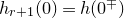 $h_{r+1}(0) = h(0^\mp)$
, then splitting in cases depending on the sign
$h_{r+1}(0) = h(0^\mp)$
, then splitting in cases depending on the sign
 $\pm$
and on whether
$\pm$
and on whether
 $y\to0$
from the right or the left, we find
$y\to0$
from the right or the left, we find
 $$ f^\triangleleft(y) - f(x) \to \begin{cases} q^k(h(0^+) - f(0)) & (y\to x^+), \\ q^k(h(0^-) - f(0)) & (y \to x^-), \end{cases} $$
as claimed. We also notice for later use that if h is continuous at zero, then (2.23) gives
 $$\begin{equation*} {\lim_{y\to x^+}} w_r(y)={\lim_{y\to x^-}} w_{r+1}(y),\quad{\lim_{y\to x^-}} w_r(y)={\lim_{y\to x^+}} w_{r+1}(y).\end{equation*}$$
2.3.3 Proof of Theorem 1.1. The differentiability of
$f^\triangleleft$
.

We argue by induction, starting from the case
 $m=1$
. Assume that
$m=1$
. Assume that
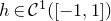 $h\in\mathcal{C}^1([-1, 1])$
and
$h\in\mathcal{C}^1([-1, 1])$
and
 $\operatorname{Re}(k)<-2$
.
$\operatorname{Re}(k)<-2$
.
By Lemma 2.7 we have that
 $w_j$
is of
$w_j$
is of
 $\mathcal{C}^1$
class on
$\mathcal{C}^1$
class on
 $[0, 1)\smallsetminus \{x, r(x)\in\{j-1,j\}\}$
(and thus on any neighborhood of irrational numbers). In particular, by (2.22), (2.16) and (2.17), it follows that
$[0, 1)\smallsetminus \{x, r(x)\in\{j-1,j\}\}$
(and thus on any neighborhood of irrational numbers). In particular, by (2.22), (2.16) and (2.17), it follows that
 $f^\triangleleft$
is differentiable on
$f^\triangleleft$
is differentiable on
 $\mathbb{R}\smallsetminus\mathbb{Q}$
. The same argument also gives that
$\mathbb{R}\smallsetminus\mathbb{Q}$
. The same argument also gives that
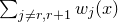 $\sum_{j\neq r,r+1} w_j(x)$
is differentiable at rationals. In particular, it suffices to show that the right and left derivatives of
$\sum_{j\neq r,r+1} w_j(x)$
is differentiable at rationals. In particular, it suffices to show that the right and left derivatives of
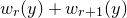 $w_r(y)+w_{r+1}(y)$
coincide at rationals. To show this, we start by observing that from the period relation (1.2), proceeding as in [Reference ZagierZag99, Equation (23)], we have
$w_r(y)+w_{r+1}(y)$
coincide at rationals. To show this, we start by observing that from the period relation (1.2), proceeding as in [Reference ZagierZag99, Equation (23)], we have
 $$ h(x+1) - h(x) =-{| {1+x} |}^{-k}h(1-1/(x+1)) ,\quad x\in\mathbb{Q}\smallsetminus\{0,-1\}. $$
In particular, taking the limit as
 $x\to 0$
, we obtain
$x\to 0$
, we obtain
 $h(1)=0$
and
$h(1)=0$
and
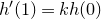 $h'( 1) = k h(0)$
. Thus, since by (1.2) we have
$h'( 1) = k h(0)$
. Thus, since by (1.2) we have
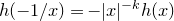 $h(-1/x)=-|x|^{-k}h(x)$
, we find
$h(-1/x)=-|x|^{-k}h(x)$
, we find
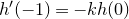 $h'(- 1)=-kh(0)$
and thus
$h'(- 1)=-kh(0)$
and thus
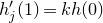 $h_j'(1)=kh(0)$
for all j. Thus, recalling that
$h_j'(1)=kh(0)$
for all j. Thus, recalling that
 $h_j(1)=0$
(and
$h_j(1)=0$
(and
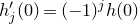 $h_j'(0)=(-1)^j h(0)$
) and observing that
$h_j'(0)=(-1)^j h(0)$
) and observing that
 $$ -k\sum_{i=0}^{r(x)} \frac{(-1)^i}{u_i(x)u_{i+1}(x)} = -k\sum_{i=0}^{r(x)-1} \frac{(-1)^i}{u_i(x)u_{i+1}(x)} - (-1)^r k,\quad x\in\mathbb{Q}\cap(0,1), $$
we obtain from (2.15) that
 \begin{equation*} w'_r(x^+)+w'_{r+1}(x^+)=w'_r(x^-) +w'_{r+1}(x^-), \quad x\in\mathbb{Q}\cap(0,1),\end{equation*}
thus giving that
 $f^\triangleleft$
is differentiable at any
$f^\triangleleft$
is differentiable at any
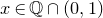 $x\in\mathbb{Q}\cap(0,1)$
. Finally, by (1.2), we see that
$x\in\mathbb{Q}\cap(0,1)$
. Finally, by (1.2), we see that
 $f^\triangleleft$
is differentiable at 0 also, with
$f^\triangleleft$
is differentiable at 0 also, with
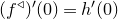 $(f^\triangleleft)'(0) = h'(0)$
. We conclude that
$(f^\triangleleft)'(0) = h'(0)$
. We conclude that
 $f^\triangleleft$
is differentiable on [0, 1), hence on
$f^\triangleleft$
is differentiable on [0, 1), hence on
 $\mathbb{R}$
by periodicity. By (1.2), its derivative satisfies, for
$\mathbb{R}$
by periodicity. By (1.2), its derivative satisfies, for
 $x\neq 0$
,
$x\neq 0$
,
 $$ h_1(x) = (f^\triangleleft)'(x) - {| {x} |}^{-k-2}(f^\triangleleft)'(-1/x), $$
where
 $h_1(x) := h'(x) - k\textrm{sgn}(x) {| {x} |}^{-k-1}f(-1/x)$
. The function
$h_1(x) := h'(x) - k\textrm{sgn}(x) {| {x} |}^{-k-1}f(-1/x)$
. The function
 $h_1$
, extended at 0 by
$h_1$
, extended at 0 by
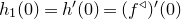 $h_1(0)=h'(0)=(f^\triangleleft)'(0)$
, is continuous on
$h_1(0)=h'(0)=(f^\triangleleft)'(0)$
, is continuous on
 $[-1, 1]$
. We can then apply the continuity property proven in § 2.3.2 to
$[-1, 1]$
. We can then apply the continuity property proven in § 2.3.2 to
 $(f^\triangleleft)'$
and deduce that
$(f^\triangleleft)'$
and deduce that
 $(f^\triangleleft)'$
is continuous on [0, 1], and hence on
$(f^\triangleleft)'$
is continuous on [0, 1], and hence on
 $\mathbb{R}$
.
$\mathbb{R}$
.
If
 $k<-2m$
and
$k<-2m$
and
 $h\in\mathcal{C}^m$
, then this argument can be iterated m times, with functions
$h\in\mathcal{C}^m$
, then this argument can be iterated m times, with functions
 $(h_n)_{n\leqslant m}$
defined inductively by
$(h_n)_{n\leqslant m}$
defined inductively by
 $$ h_0(x) = h(x), \quad h_{n+1}(x) = h_n'(x) - (k+2n) \textrm{sgn}(x) {| {x} |}^{-k-2n-1} (f^\triangleleft)^{(n)}(-1/x). $$
2.3.4 Proof of Theorem 1.2. Extending f when h is unbounded.
We now justify Theorem 1.2. We assume that h satisfies (1.5). First note that, due to the fact that periodicity is assumed separately on
 $\mathbb{R}_+$
and
$\mathbb{R}_+$
and
 $\mathbb{R}_-$
, we have the following variant of (2.1),
$\mathbb{R}_-$
, we have the following variant of (2.1),
 $$ f(x) = \sum_{j=0}^{r-1} \bigg(\prod_{i=0}^{j-1} T^i(x)\bigg)^{\!{-}k} h((-1)^j T^j(x)) + q^k f((-1)^r). $$
Lemma 2.9. Let
 $\delta>0$
be such that the hypothesis (1.5) holds. Then f has the property
$\delta>0$
be such that the hypothesis (1.5) holds. Then f has the property
 $\mathscr{S}(1+\delta)$
.
$\mathscr{S}(1+\delta)$
.
Proof. Let
 $x = [b_0; b_1, b_2, \dotsc] \in \mathfrak{T}(m^{1+\delta})$
. By periodicity we can assume
$x = [b_0; b_1, b_2, \dotsc] \in \mathfrak{T}(m^{1+\delta})$
. By periodicity we can assume
 $x\in[0,1)$
, that is
$x\in[0,1)$
, that is
 $b_0=0$
. If
$b_0=0$
. If
 $U:[0,1)\to\mathbb{R}$
is the inverse branch of
$U:[0,1)\to\mathbb{R}$
is the inverse branch of
 $T^m$
, given by
$T^m$
, given by
 $U(y) = [0; b_1, \dotsc, b_m+ y]$
, then any
$U(y) = [0; b_1, \dotsc, b_m+ y]$
, then any
 $x'\in V(m^{1+\delta}, m, x)$
is in the range of U. By [Reference Marmi, Moussa and YoccozMMY97, Proposition 1.14], we have
$x'\in V(m^{1+\delta}, m, x)$
is in the range of U. By [Reference Marmi, Moussa and YoccozMMY97, Proposition 1.14], we have
 $$ \|(T^j\circ U)'\|_\infty = \sup_{y\in [0, 1]} \prod_{i=j}^{m-1} {| {T^i(U(y))} |}^2 \ll \varpi^{-2(m-j)}$$
uniformly for
 $0\leqslant j < m$
, and therefore, for any
$0\leqslant j < m$
, and therefore, for any
 $x', x'' \in V(m^{1+\delta}, m, x)$
,
$x', x'' \in V(m^{1+\delta}, m, x)$
,
 \begin{equation} {| {T^j(x') - T^j(x'')} |} \ll \varpi^{-2(m-j)} \end{equation}
for
 $j<m$
. We note also that
$j<m$
. We note also that
 $T^j(x') \asymp T^j(x)$
for
$T^j(x') \asymp T^j(x)$
for
 $x' \in V(m^{1+\delta}, m, x)$
and
$x' \in V(m^{1+\delta}, m, x)$
and
 $j<m$
, with a uniform constant, and that the condition
$j<m$
, with a uniform constant, and that the condition
 $T^j(x') \gg \min(m^{-1-\delta}, j^{-1} (\log j)^{-2})$
holds uniformly over j. Finally, for any
$T^j(x') \gg \min(m^{-1-\delta}, j^{-1} (\log j)^{-2})$
holds uniformly over j. Finally, for any
 $x'\in V(m^{1+\delta}, m, x)$
, the condition
$x'\in V(m^{1+\delta}, m, x)$
, the condition
 $r(x')\geqslant m$
implies
$r(x')\geqslant m$
implies
 $\operatorname{Den}(x') \geqslant \varpi^m$
by virtue of (1.16) (with
$\operatorname{Den}(x') \geqslant \varpi^m$
by virtue of (1.16) (with
 $j=r(x')$
).
$j=r(x')$
).
Given
 $x\in \mathfrak{T}(m^{1+\delta})$
and
$x\in \mathfrak{T}(m^{1+\delta})$
and
 $x'\in V(m^{1+\delta}, m, x)$
, with the same notation as in § 2.3.1 we have
$x'\in V(m^{1+\delta}, m, x)$
, with the same notation as in § 2.3.1 we have
 \begin{equation*} f(x') = \sum_{0\leqslant j < m/2} w_j(x') + O\bigg(\operatorname{Den}(x)^{\operatorname{Re}(k)} + \sum_{j\geqslant m/2} \varpi^{\operatorname{Re}(k)j} \sup_{{| {y} |}\gg \min(m^{-1-\delta}, j^{-1}(\log j)^{-2})} {| {h(y)} |}\bigg). \end{equation*}
By our hypothesis (1.5), the second sum is
 $\ll \sum_{j\geqslant m/2} \varpi^{\operatorname{Re}(k) j}({e}^{j^{1-\delta}(\log j)^2} + {e}^{O(m^{1-\delta^2})}) \ll \varpi^{\operatorname{Re}(k)m/3}$
, and therefore
$\ll \sum_{j\geqslant m/2} \varpi^{\operatorname{Re}(k) j}({e}^{j^{1-\delta}(\log j)^2} + {e}^{O(m^{1-\delta^2})}) \ll \varpi^{\operatorname{Re}(k)m/3}$
, and therefore
 \begin{equation} f(x') = \sum_{0\leqslant j < m/2} w_j(x') + O(\varpi^{\operatorname{Re}(k) m/3}). \end{equation}
We now let
 $x', x'' \in V(m^{1+\delta}, m, x)$
be given. Taking differences in the expansion (2.25), we obtain
$x', x'' \in V(m^{1+\delta}, m, x)$
be given. Taking differences in the expansion (2.25), we obtain
 $$ {| {f(x') - f(x'')} |} \ll \sum_{0\leqslant j < m/2} {| {w_j(x') - w_j(x'')} |} + \varpi^{\operatorname{Re}(k)m/3}. $$
Denote temporarily
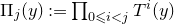 $ \Pi_j(y) := \prod_{0\leqslant i < j} T^i(y)$
, which is also
$ \Pi_j(y) := \prod_{0\leqslant i < j} T^i(y)$
, which is also
 $u_j(y) / u_0(y)$
in the notation of § 1.4. By the definition (2.12), (2.19) of
$u_j(y) / u_0(y)$
in the notation of § 1.4. By the definition (2.12), (2.19) of
 $w_j$
, splitting the difference in
$w_j$
, splitting the difference in
 $w_j(x') - w_j(x'')$
, we get
$w_j(x') - w_j(x'')$
, we get
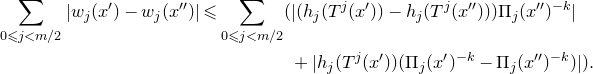 \begin{align*} \sum_{0\leqslant j < m/2} {| {w_j(x') - w_j(x'')} |} \leqslant \sum_{0\leqslant j < m/2} (&{| {(h_j(T^j(x')) - h_j(T^j(x''))) \Pi_j(x'')^{-k}} |} \\ & + {| {h_j(T^j(x'))(\Pi_j(x')^{-k} - \Pi_j(x'')^{-k})} |} ). \end{align*}
Regarding the first term inside the sum, the bound (2.24) and our hypothesis (1.5), applied with some value of
 $\varepsilon \asymp m^{-1-\delta}$
, give
$\varepsilon \asymp m^{-1-\delta}$
, give
 ${| {h_j(T^j(x')) - h_j(T^j(x''))} |} = o(1)$
as
${| {h_j(T^j(x')) - h_j(T^j(x''))} |} = o(1)$
as
 $m\to \infty$
uniformly for all
$m\to \infty$
uniformly for all
 $j<m/2$
. By the bound (1.16), we further have
$j<m/2$
. By the bound (1.16), we further have
 $\Pi_j(y) \ll \varpi^{-j}$
uniformly for
$\Pi_j(y) \ll \varpi^{-j}$
uniformly for
 $y\in[0, 1]$
and
$y\in[0, 1]$
and
 $j\geqslant 0$
, and therefore
$j\geqslant 0$
, and therefore
 $$ \sum_{0\leqslant j < m/2} {| {(h_j(T^j(x')) - h_j(T^j(x''))) \Pi_j(x'')^{-k}} |} \ll o(1) \times \sum_{j\geqslant 0} \varpi^{j \operatorname{Re}(k)} = o(1) $$
as
 $m \to \infty$
. Regarding the second term, we have, as above,
$m \to \infty$
. Regarding the second term, we have, as above,
 $h_j(T^j(x')) \ll {e}^{m^{1-\delta^2}} + {e}^{j^{1-\delta} (\log j)^2}$
for all
$h_j(T^j(x')) \ll {e}^{m^{1-\delta^2}} + {e}^{j^{1-\delta} (\log j)^2}$
for all
 $j\geqslant 0$
. We use the inequality
$j\geqslant 0$
. We use the inequality
 $u^{-k}-v^{-k} \ll_k {| {u-v} |}^{\min(1, -k)}$
, valid for
$u^{-k}-v^{-k} \ll_k {| {u-v} |}^{\min(1, -k)}$
, valid for
 $0\leqslant u, v \leqslant 1$
, which gives in our case
$0\leqslant u, v \leqslant 1$
, which gives in our case
 $$ \Pi_j(x')^{-k} - \Pi_j(x'')^{-k} \ll {| {\Pi_j(x') - \Pi_j(x'')} |}^{\min(-k, 1)}. $$
Splitting the difference, we have
 \begin{align*} {| {\Pi_j(x') - \Pi_j(x'')} |} \leqslant {}& \sum_{0\leqslant i \leqslant j} \Pi_{i-1}(x') \Pi_{j-i-1}(T^{i+1}(x'')) {| {T^i(x') - T^i(x'')} |} \\ \ll {}& \sum_{0\leqslant i \leqslant j} \varpi^{-i} \times \varpi^{-(j-i)} \times \varpi^{-2(m - i)} \\ \ll {}& \varpi^{-2m+j} \end{align*}
using our bound (2.24) and thus we conclude that
 \begin{align*} & \sum_{0\leqslant j < m/2} {| {h_j(T^j(x'))(\Pi_j(x')^{-k} - \Pi_j(x'')^{-k})} |} \\ &\quad \ll \varpi^{-2m \min(-k, 1)} \sum_{j\geqslant 0} \varpi^{j\min(-k, 1)}({e}^{O(m^{1-\delta^2})} + {e}^{O(j^{1-\delta} (\log j)^2)}) \\&\quad \ll \varpi^{-m \min(-k, 1)/2}, \end{align*}
which tends to 0 as
 $m\to \infty$
. Grouping our bounds, we deduce
$m\to \infty$
. Grouping our bounds, we deduce
 $\Delta_{1+\delta}(m) \to 0$
when
$\Delta_{1+\delta}(m) \to 0$
when
 $m\to\infty$
, as claimed.
$m\to\infty$
, as claimed.
We now turn to the proof of Theorem 1.2. Consider
 $X = (\mathbb{R}\smallsetminus\mathbb{Q}) \cap \mathfrak{S}$
, where
$X = (\mathbb{R}\smallsetminus\mathbb{Q}) \cap \mathfrak{S}$
, where
 $\mathfrak{S}$
is defined in Lemma 2.2, and let
$\mathfrak{S}$
is defined in Lemma 2.2, and let
 $x\in X$
. In particular,
$x\in X$
. In particular,
 $x\in \mathfrak{T}(B)$
for some
$x\in \mathfrak{T}(B)$
for some
 $B>0$
, and therefore so do the convergents
$B>0$
, and therefore so do the convergents
 $x_j$
of x. Summarizing, we have
$x_j$
of x. Summarizing, we have
 $x_j\in \mathbb{Q}\cap\mathfrak{T}(B)$
for all j, and
$x_j\in \mathbb{Q}\cap\mathfrak{T}(B)$
for all j, and
 $x_j \to x$
as
$x_j \to x$
as
 $j\to\infty$
. Since f has the property
$j\to\infty$
. Since f has the property
 $\mathscr{S}(1+\delta)$
by Lemma 2.9, the limit
$\mathscr{S}(1+\delta)$
by Lemma 2.9, the limit
 $f^\triangleleft(x) := f^*(x) = \lim_{j\to\infty} f(x_j)$
in (2.9) exists.
$f^\triangleleft(x) := f^*(x) = \lim_{j\to\infty} f(x_j)$
in (2.9) exists.
Moreover, for any
 $\varepsilon$
, by Lemma 2.2 we can find
$\varepsilon$
, by Lemma 2.2 we can find
 $B>0$
such that
$B>0$
such that
 $X_\varepsilon :=(\mathbb{R}\smallsetminus\mathbb{Q}) \cap \mathfrak{T}(B) \subset X$
satisfies
$X_\varepsilon :=(\mathbb{R}\smallsetminus\mathbb{Q}) \cap \mathfrak{T}(B) \subset X$
satisfies
 $\nu(X_\varepsilon\cap [0, 1])\geqslant 1-\varepsilon$
. This set is also trivially invariant by
$\nu(X_\varepsilon\cap [0, 1])\geqslant 1-\varepsilon$
. This set is also trivially invariant by
 $x\mapsto x+1$
. Let
$x\mapsto x+1$
. Let
 $y\in X_\varepsilon$
and
$y\in X_\varepsilon$
and
 $\eta>0$
be arbitrary. We pick an integer
$\eta>0$
be arbitrary. We pick an integer
 $m\geqslant B^{1/(1+\delta)}$
such that the right-hand side of (2.10) has modulus at most
$m\geqslant B^{1/(1+\delta)}$
such that the right-hand side of (2.10) has modulus at most
 $\delta$
. Having chosen m, and since
$\delta$
. Having chosen m, and since
 $y\not\in\mathbb{Q}$
, we may find
$y\not\in\mathbb{Q}$
, we may find
 $\xi>0$
such that any number
$\xi>0$
such that any number
 $x\in (\mathbb{R}\smallsetminus\mathbb{Q})\cap[y-\xi, y+\xi]$
satisfies
$x\in (\mathbb{R}\smallsetminus\mathbb{Q})\cap[y-\xi, y+\xi]$
satisfies
 $b_j(x) = b_j(y)$
for
$b_j(x) = b_j(y)$
for
 $j\leqslant m$
. Now let
$j\leqslant m$
. Now let
 $x\in X_\varepsilon \cap[y-\xi, y+\xi]$
be arbitrary. Then
$x\in X_\varepsilon \cap[y-\xi, y+\xi]$
be arbitrary. Then
 $x\in \mathfrak{T}(B)$
by definition, and therefore the formula (2.10) gives
$x\in \mathfrak{T}(B)$
by definition, and therefore the formula (2.10) gives
 ${| {f^\triangleleft(x) - f^\triangleleft(y)} |} \leqslant \eta$
. We have thus proven that
${| {f^\triangleleft(x) - f^\triangleleft(y)} |} \leqslant \eta$
. We have thus proven that
 $f^\triangleleft|_{X_\varepsilon}$
is continuous at y with the restricted topology, as claimed.
$f^\triangleleft|_{X_\varepsilon}$
is continuous at y with the restricted topology, as claimed.
2.4 The case of
$\operatorname{Re}(k)>0$
.

2.4.1 Proofs of Theorems 1.4 and 1.5. The domain and continuity of
$f^\triangleright$
.

For the purpose of studying the example of the Kontsevich function (1.12), it will be convenient to generalize the period relations to
 \begin{equation} \begin{cases} f(x+1) = \vartheta f(x) & (x\in \mathbb{Q}), \\ h(x) = f(x) - \vartheta^{\pm 3} {| {x} |}^{-k} f(-1/x) & (\pm x \in \mathbb{Q}_{>0}), \end{cases}\end{equation}
where
 $\vartheta$
is some fixed root of unity. Define
$\vartheta$
is some fixed root of unity. Define
 \begin{align} \vartheta_j = \vartheta_j(b_1, b_2, \dotsc) = \begin{cases} \vartheta^{\sum_{i=1}^j (-1)^i b_i} & (j\text{ even}), \\ \vartheta^{3+\sum_{i=1}^j (-1)^i b_i} & (j\text{ odd}), \end{cases}\end{align}
where
 $b_1, b_2, \dotsc$
are integers. By arguing in the same way as (2.2), we find for
$b_1, b_2, \dotsc$
are integers. By arguing in the same way as (2.2), we find for
 $x = [0; b_1, \dotsc, b_r]$
that
$x = [0; b_1, \dotsc, b_r]$
that
 \begin{equation} f(x) = \sum_{j=0}^{r-1} \vartheta_j\, \bigg(\frac{u_j}{u_0}\bigg)^{\!{-}k} h\bigg((-1)^j \frac{u_{j+1}}{u_j}\bigg) + \vartheta_r u_0^k f(0).\end{equation}
Note that by the period relation, we have
 $$ h((-1)^r) = (\vartheta^{(-1)^r} - \vartheta^{3(-1)^r+(-1)^{r+1}}) f(0), $$
which confirms that the expression (2.28) holds for
 $x = [0; b_1, \dotsc, b_r]$
regardless of whether this expansion is canonical (
$x = [0; b_1, \dotsc, b_r]$
regardless of whether this expansion is canonical (
 $b_r>1$
if
$b_r>1$
if
 $r>1$
) or not. Similarly to (2.4), we may then work with r odd, for which we observe that
$r>1$
) or not. Similarly to (2.4), we may then work with r odd, for which we observe that
 $$ \vartheta_{r-j}(b_1, \dotsc, b_r)\vartheta_{j}(b_r, \dotsc, b_1) = \vartheta_{r}(b_1, \dotsc, b_r). $$
Changing j to
 $r-j$
in the sum (2.28), and using the notation (1.17), we deduce that for
$r-j$
in the sum (2.28), and using the notation (1.17), we deduce that for
 $x = [0; b_1, \dotsc, b_r]$
, r odd, we have
$x = [0; b_1, \dotsc, b_r]$
, r odd, we have
 \begin{equation} \vartheta_r^{-1}(x) q^{-k} f(x) = \Psi(\overline{x}),\end{equation}
where now
 $\Psi(y)$
is defined for
$\Psi(y)$
is defined for
 $y = [0; c_1, \dotsc, c_r]$
, r odd, as
$y = [0; c_1, \dotsc, c_r]$
, r odd, as
 \begin{equation} \Psi(y) = \sum_{j=1}^r \vartheta_j^{-1}(y) v_j(y)^{-k} h\bigg((-1)^j \frac{v_{j-1}(y)}{v_j(y)}\bigg) + f(0),\end{equation}
where, whenever the expansion
 $x = [0;b_1, \dotsc, b_r]$
is clear from the context, we denote
$x = [0;b_1, \dotsc, b_r]$
is clear from the context, we denote
 \begin{equation} \vartheta_j(x) = \vartheta_j(b_1, \dotsc),\end{equation}
but this quantity in fact depends on the tuple
 $(b_j)$
representing x.
$(b_j)$
representing x.
In the case of
 $\operatorname{Re}(k)>0$
and
$\operatorname{Re}(k)>0$
and
 $h(x)=O(|x|^{-\operatorname{Re}(k)})$
for
$h(x)=O(|x|^{-\operatorname{Re}(k)})$
for
 $x\in[-1,1]\smallsetminus\{0\}$
, the existence of
$x\in[-1,1]\smallsetminus\{0\}$
, the existence of
 $f^\triangleright$
for all
$f^\triangleright$
for all
 $x\in\mathbb{R}$
is straightforward. Indeed, by (2.28) we have
$x\in\mathbb{R}$
is straightforward. Indeed, by (2.28) we have
 \begin{align} f^\triangleright(x)=\begin{cases} \Psi( x) & \text{if }x\in\mathbb{Q}, \\ {\displaystyle \lim_{\mathbb{Q}\ni y\to x}\Psi( y)} & \text{if }x\notin\mathbb{Q}, \end{cases}\end{align}
where the limit exists by virtue of the fact that the sum in (2.28) is uniformly convergent and for each j,
 $v_j(y)$
depends only on finitely many of the functions
$v_j(y)$
depends only on finitely many of the functions
 $y \mapsto b_j(y) = {\lfloor {1/T^{j-1}(y)} \rfloor}$
which are locally constant at irrationals. Note that for irrational
$y \mapsto b_j(y) = {\lfloor {1/T^{j-1}(y)} \rfloor}$
which are locally constant at irrationals. Note that for irrational
 $x=[0;c_1,c_2,\ldots]$
we simply have
$x=[0;c_1,c_2,\ldots]$
we simply have
 \begin{equation} f^\triangleright(x)=\sum_{j=1}^{\infty}\vartheta_j^{-1}v_{j}^{-k} h\bigg((-1)^{j-1}\frac{v_{j-1}}{v_{j}}\bigg)+f(0).\end{equation}
The continuity of
 $f^\triangleright$
on
$f^\triangleright$
on
 $\mathbb{R}\smallsetminus\mathbb{Q}$
when
$\mathbb{R}\smallsetminus\mathbb{Q}$
when
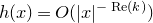 $h(x)=O(|x|^{-\operatorname{Re}(k)})$
is immediate from (2.33). Suppose
$h(x)=O(|x|^{-\operatorname{Re}(k)})$
is immediate from (2.33). Suppose
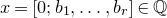 $x=[0;b_1,\ldots,b_r]\in\mathbb{Q}$
with r odd. If
$x=[0;b_1,\ldots,b_r]\in\mathbb{Q}$
with r odd. If
 $x'\to x^-$
with x’ sufficiently close to x, then we have
$x'\to x^-$
with x’ sufficiently close to x, then we have
 $x'=[0;b_1,\ldots,b_r,b',b_{r+2}',\ldots]$
with
$x'=[0;b_1,\ldots,b_r,b',b_{r+2}',\ldots]$
with
 $b'\to\infty$
. It follows immediately from the definition that
$b'\to\infty$
. It follows immediately from the definition that
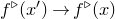 $f^\triangleright(x')\to f^\triangleright(x)$
if
$f^\triangleright(x')\to f^\triangleright(x)$
if
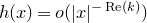 $h(x)=o(|x|^{-\operatorname{Re}(k)})$
as
$h(x)=o(|x|^{-\operatorname{Re}(k)})$
as
 $x\to0$
, and so under this assumption
$x\to0$
, and so under this assumption
 $f^\triangleright$
is continuous at x from the left. Next, let
$f^\triangleright$
is continuous at x from the left. Next, let
 $x'\to x^+$
, then if
$x'\to x^+$
, then if
 $b_r>1$
we have
$b_r>1$
we have
 $x'=[0;b_1,\ldots,b_r-1,1,b',b'_{r+2},\ldots]$
with
$x'=[0;b_1,\ldots,b_r-1,1,b',b'_{r+2},\ldots]$
with
 $b'\to\infty$
. Note that
$b'\to\infty$
. Note that
 $$ \frac{v_{r-1}(x)}{v_{r}(x)} = \overline x, \quad \frac{v_{r-1}(x')}{v_r(x')} = \frac{v_{r-1}(x)}{v_r(x)-v_{r-1}(x)} = \frac{\overline x}{1-\overline x}, \quad \frac{v_{r}(x')}{v_{r+1}(x')}=1-\overline x. $$
Then, under the hypothesis
 $h(x)=o(|x|^{-\operatorname{Re}(k)})$
, by (2.30) and the relations (2.26), we obtain
$h(x)=o(|x|^{-\operatorname{Re}(k)})$
, by (2.30) and the relations (2.26), we obtain
 \begin{align*} f^\triangleright(x')-f^\triangleright(x) = {}& \vartheta_r^{-1} q^{-k} \bigg(\vartheta^{-1} (1-\overline x)^{-k} h\bigg(\frac{\overline x}{1-\overline x}\bigg) + \vartheta h(\overline x-1) - h(\overline x)\bigg) + o(1) \\ = {}& \vartheta_r^{-1} q^{-k} \bigg( \vartheta^{-1}(1-\overline x)^{-k}f\bigg(\frac{\overline x}{1-\overline x}\bigg) + \vartheta h(\overline x - 1) - f(\overline x) \bigg)+o(1) \\ = {}& o(1)\end{align*}
as
 $b'\to\infty$
. If
$b'\to\infty$
. If
 $b_r=1$
, then
$b_r=1$
, then
 $x'=[0;b_1,\ldots,b_{r-1}+1,b',b'_{r+1},\ldots]$
with
$x'=[0;b_1,\ldots,b_{r-1}+1,b',b'_{r+1},\ldots]$
with
 $b'\to\infty$
. We then obtain in a similar way
$b'\to\infty$
. We then obtain in a similar way
 \begin{align*} f^\triangleright(x')-f^\triangleright(x) = {}& \vartheta_r^{-1}q^{-k}\bigg( \vartheta h(\overline x - 1) - h(\overline x) - \vartheta^2 (\overline x)^{-k} h\bigg(\frac{\overline x - 1}{\overline x}\bigg) \bigg) + o(1) \\ = {}& o(1),\end{align*}
which goes to 0 as
 $x'\to x^+$
, and concludes the proof that
$x'\to x^+$
, and concludes the proof that
 $f^\triangleright$
is continuous on
$f^\triangleright$
is continuous on
 $\mathbb{R}$
. This proves the first part of Theorem 1.4.
$\mathbb{R}$
. This proves the first part of Theorem 1.4.
Assume now that f is not (twisted) periodic, but instead satisfies
 $f(x) = \vartheta f(x+1)$
only for
$f(x) = \vartheta f(x+1)$
only for
 $x \in \mathbb{Q}\smallsetminus[-1, 0]$
, and that h satisfies
$x \in \mathbb{Q}\smallsetminus[-1, 0]$
, and that h satisfies
 $h(x)=O({e}^{|x|^{-1+\delta}})$
for some
$h(x)=O({e}^{|x|^{-1+\delta}})$
for some
 $\delta>0$
. In this situation, we use Proposition 2.5 to extend
$\delta>0$
. In this situation, we use Proposition 2.5 to extend
 $\Psi$
.
$\Psi$
.
Lemma 2.10. Let
 $\delta>0$
, and assume that f satisfies
$\delta>0$
, and assume that f satisfies
 $$\begin{equation*} \begin{cases} f(x+1) = \vartheta f(x) & (x\in \mathbb{Q}\smallsetminus[-1, 0]), \\ h(x) = f(x) - \vartheta^{\pm 3} {| {x} |}^{-k} f(-1/x) & (\pm x \in \mathbb{Q}_{>0}), \end{cases} \end{equation*}$$
and that the map h defined through (1.2) satisfies
 $h(x) = O({e}^{|x|^{-1+\delta}})$
. Then the formula (2.29) holds with
$h(x) = O({e}^{|x|^{-1+\delta}})$
. Then the formula (2.29) holds with
 $$ \Psi(y) := \sum_{j=1}^r \vartheta_j^{-1}(y) v_j(y)^{-k} h\bigg((-1)^j \frac{v_{j-1}(y)}{v_j(y)}\bigg) + \vartheta^{-1} f(-1) \quad (y=[0;c_1, \dotsc, c_r]; r\text{ odd}), $$
and the map
 $\Psi$
has the property
$\Psi$
has the property
 $\mathscr{S}(1+\delta)$
.
$\mathscr{S}(1+\delta)$
.
Proof. The verification that Equations (2.29) and (2.30) hold, with f(0) replaced with
 $\vartheta^{-1}f(-1)$
, is straightforward. Let
$\vartheta^{-1}f(-1)$
, is straightforward. Let
 $B = m^{1+\delta}$
,
$B = m^{1+\delta}$
,
 $x\in \mathfrak{T}(B)$
and
$x\in \mathfrak{T}(B)$
and
 $x', x'' \in V(B, m, x)$
. Note, in particular, that
$x', x'' \in V(B, m, x)$
. Note, in particular, that
 $b_j(x') = b_j(x'')$
for all
$b_j(x') = b_j(x'')$
for all
 $j\leqslant m$
, and therefore also
$j\leqslant m$
, and therefore also
 $v_j(x') = v_j(x'')$
and
$v_j(x') = v_j(x'')$
and
 $\vartheta_j(x') = \vartheta_j(x'')$
. We deduce
$\vartheta_j(x') = \vartheta_j(x'')$
. We deduce
 $$ {| {\Psi(x') - \Psi(x'')} |} \leqslant \sum_{j=m+1}^{r(x')} v_j(x')^{-\operatorname{Re}(k)} {\bigg| {h\bigg(\!(-1)^j \frac{v_{j-1}(x')}{v_j(x')}\bigg)} \bigg|} + \sum_{j=m+1}^{r(x'')} v_j(x'')^{-\operatorname{Re}(k)} {\bigg| {h\bigg(\!(-1)^j \frac{v_{j-1}(x'')}{v_j(x'')}\bigg)}\! \bigg|}. $$
Since
 $x'\in\mathfrak{T}(B)$
, we also have
$x'\in\mathfrak{T}(B)$
, we also have
 $v_{j-1}(x') / v_j(x') \gg 1/b_j(x') \gg j^{-1}(\log j)^{-2} + B^{-1}$
. The same holds for x”. By our hypothesis on h, and combining this with (1.18), we deduce
$v_{j-1}(x') / v_j(x') \gg 1/b_j(x') \gg j^{-1}(\log j)^{-2} + B^{-1}$
. The same holds for x”. By our hypothesis on h, and combining this with (1.18), we deduce
 $$ {| {\Psi(x') - \Psi(x'')} |} \ll \sum_{j\geqslant m+1} \varpi^{-j \operatorname{Re}(k)} ({e}^{O(j^{1-\delta}(\log j)^2)} + {e}^{O(m^{1-\delta^2})}) \ll \varpi^{-m \operatorname{Re}(k)/2}, $$
which tends to 0 as
 $m\to \infty$
, uniformly in x, x’, x”. This shows the property
$m\to \infty$
, uniformly in x, x’, x”. This shows the property
 $\mathscr{S}(1+\delta)$
for
$\mathscr{S}(1+\delta)$
for
 $\Psi$
.
$\Psi$
.
Letting
 $f^\triangleright(x) := \Psi^*(x)$
with the notation of Proposition 2.5, the deduction Theorem 1.5 follows by arguments identical to those of § 2.3.4, which were used to prove Theorem 1.2.
$f^\triangleright(x) := \Psi^*(x)$
with the notation of Proposition 2.5, the deduction Theorem 1.5 follows by arguments identical to those of § 2.3.4, which were used to prove Theorem 1.2.
2.4.2 Proof of Theorem 1.4. The differentiability of
$f^\triangleright$
.

We assume here the hypotheses of Theorem 1.4, in particular, that
 $h(x)=O(|x|^{-\operatorname{Re}(k)})$
for
$h(x)=O(|x|^{-\operatorname{Re}(k)})$
for
 $0<|x|<1$
. Let
$0<|x|<1$
. Let
 $X = \mathfrak{S}$
be as in Lemma 2.2, let
$X = \mathfrak{S}$
be as in Lemma 2.2, let
 $\varepsilon>0$
and suppose
$\varepsilon>0$
and suppose
 $x=[0;b_1,b_2,\ldots] \in \mathfrak{S}$
. Let
$x=[0;b_1,b_2,\ldots] \in \mathfrak{S}$
. Let
 $m := m(x,\varepsilon)$
be as in § 2.3.1. Let
$m := m(x,\varepsilon)$
be as in § 2.3.1. Let
 $x'\in(0,1)$
be such that
$x'\in(0,1)$
be such that
 $|x-x'|<\varepsilon$
, so that
$|x-x'|<\varepsilon$
, so that
 $x'=[b_1,\ldots,b_m,b_{m+1}',\ldots]$
. Let
$x'=[b_1,\ldots,b_m,b_{m+1}',\ldots]$
. Let
 $n\geqslant m$
be the least integer such that
$n\geqslant m$
be the least integer such that
 $b_{n+1}\neq b_{n+1}'$
. We write
$b_{n+1}\neq b_{n+1}'$
. We write
 $x=[0;b_1,\ldots,b_n,z]$
and
$x=[0;b_1,\ldots,b_n,z]$
and
 $x'=[0;b_1,\ldots,b_n,z']$
with
$x'=[0;b_1,\ldots,b_n,z']$
with
 $z=[b_{n+1};b_{n+2},\ldots]$
,
$z=[b_{n+1};b_{n+2},\ldots]$
,
 $z'=[b'_{n+1};b'_{n+2},\ldots]$
(and
$z'=[b'_{n+1};b'_{n+2},\ldots]$
(and
 $b_{n+1}\neq b_{n+1}'$
by hypothesis). By standard properties of continued fractions, we have
$b_{n+1}\neq b_{n+1}'$
by hypothesis). By standard properties of continued fractions, we have
 \begin{align*} |x-x'|=\frac{|z-z'|}{(z v_n+v_{n-1})(z' v_n+v_{n-1})}.\end{align*}
This is
 $\gg b_{n+1}^{-2}v_n^{-2}$
, unless
$\gg b_{n+1}^{-2}v_n^{-2}$
, unless
 $b_{n+1}-b_{n+1}'$
is equal to 1 or
$b_{n+1}-b_{n+1}'$
is equal to 1 or
 $-1$
. In the first case we have
$-1$
. In the first case we have
 $z-z'=1+1/({b_{n+2}+y})-1/({b_{n+2}'+y'})\geqslant b_{n+2}^{-1}$
for some
$z-z'=1+1/({b_{n+2}+y})-1/({b_{n+2}'+y'})\geqslant b_{n+2}^{-1}$
for some
 $0\leqslant y,y'\leqslant1$
. In the second case we have
$0\leqslant y,y'\leqslant1$
. In the second case we have
 $z'-z=1-1/({b_{n+2}+y})+1/({b_{n+2}'+y'})\geqslant y/2\geqslant -(b_{n+3}+1)^{-1}$
. Since
$z'-z=1-1/({b_{n+2}+y})+1/({b_{n+2}'+y'})\geqslant y/2\geqslant -(b_{n+3}+1)^{-1}$
. Since
 $x\in \mathfrak{S}$
, in all cases we have
$x\in \mathfrak{S}$
, in all cases we have
 $\varepsilon>|x-x'|\gg_x v_{n}^{-2} n^{-3}(\log n)^{-6} \gg v_n^{-2} (\log v_n)^{-4}$
.
$\varepsilon>|x-x'|\gg_x v_{n}^{-2} n^{-3}(\log n)^{-6} \gg v_n^{-2} (\log v_n)^{-4}$
.
Finally, we have
 \begin{align*} f^\triangleright(x)-f^\triangleright(x')\ll \sum_{j\geqslant {n+1}}\frac{1}{v_{j-1}^{\operatorname{Re}(k)}}+\sum_{j\geqslant {n+1}}\frac{1}{v_{j-1}^{\prime\,\operatorname{Re}(k)}} \ll v_n^{-\operatorname{Re}(k)} \ll_x \varepsilon^{\operatorname{Re}(k)/2}|\log \varepsilon|^{\operatorname{Re}(k)}\end{align*}
and so it follows that
 $f^\triangleright$
is locally
$f^\triangleright$
is locally
 $\alpha$
-Hölder continuous at x, for any
$\alpha$
-Hölder continuous at x, for any
 $\alpha<\frac12\operatorname{Re}(k)$
. This completes the proof of Theorem 1.4.
$\alpha<\frac12\operatorname{Re}(k)$
. This completes the proof of Theorem 1.4.
3. Limiting distributions of quantum modular forms
3.1 Convergence in distribution
3.1.1 Almost sure stability of the CF expansion.
First we need the following lemmas.
Lemma 3.1. Let
 $q\geqslant2$
and let
$q\geqslant2$
and let
 $$ \mathfrak{A}_q:=\{0\leqslant a<q\mid (a,q)=1: a/q \in \mathfrak{T}((\log q)(\log\log q)^2)\}. $$
Then
 $|\mathfrak{A}_q|=\varphi(q)(1+o(1))$
as
$|\mathfrak{A}_q|=\varphi(q)(1+o(1))$
as
 $q\to\infty$
, where
$q\to\infty$
, where
 $\varphi$
denotes Euler’s totient function.
$\varphi$
denotes Euler’s totient function.
Proof. This is a special case of [Reference RukavishnikovaRuk06].
Lemma 3.2. Let
 $q\geqslant2$
and let
$q\geqslant2$
and let
 $$ \mathfrak{T}_{q}:= ([0,1)\smallsetminus\mathbb{Q}) \cap \mathfrak{T}((\log q)(\log\log q)^2).$$
Then
 $\nu(\mathfrak{T}_q)=1+o(1)$
as
$\nu(\mathfrak{T}_q)=1+o(1)$
as
 $q\to\infty$
.
$q\to\infty$
.
Proof. This is a consequence of Lemma 2.2 with
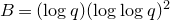 $B=(\log q)(\log\log q)^2$
.
$B=(\log q)(\log\log q)^2$
.
We can now deduce the following two lemmas, which show that
 $f^\triangleright$
and
$f^\triangleright$
and
 $f^\triangleleft$
can be well approximated by their values at suitable close-by rationals. Here again, we will obtain this as a consequence of the property
$f^\triangleleft$
can be well approximated by their values at suitable close-by rationals. Here again, we will obtain this as a consequence of the property
 $\mathscr{S}(\lambda)$
for some
$\mathscr{S}(\lambda)$
for some
 $\lambda>1$
.
$\lambda>1$
.
Lemma 3.3. Suppose that there exists
 $\lambda>1$
such that
$\lambda>1$
such that
 $f:\mathbb{Q}\to\mathbb{C}$
has the property
$f:\mathbb{Q}\to\mathbb{C}$
has the property
 $\mathscr{S}(\lambda)$
. Then the map
$\mathscr{S}(\lambda)$
. Then the map
 $f^*$
defined in Proposition 2.5 satisfies
$f^*$
defined in Proposition 2.5 satisfies
 \begin{equation} f^*(a/q) = f^*(x) + o(1) \quad \forall a\in \mathfrak{A}_q, \quad \forall x\in \bigg(\frac {a-q^{1/4}}q, \frac {a+q^{1/4}}q\bigg) \cap \bigg(\mathfrak{T}_q \cup \frac1q \mathfrak{A}_q\bigg) \end{equation}
as
 $q\to\infty$
, uniformly for a and x within the stated sets.
$q\to\infty$
, uniformly for a and x within the stated sets.
Proof. Let
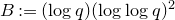 $B := (\log q)(\log\log q)^2$
. We assume first
$B := (\log q)(\log\log q)^2$
. We assume first
 $x\in(a/q, (a+q^{1/4})/q)$
, and we let
$x\in(a/q, (a+q^{1/4})/q)$
, and we let
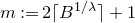 $m:=2\lceil B^{1/\lambda}\rceil+1$
, so that, in particular,
$m:=2\lceil B^{1/\lambda}\rceil+1$
, so that, in particular,
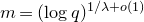 $m=(\log q)^{1/\lambda+o(1)}$
as
$m=(\log q)^{1/\lambda+o(1)}$
as
 $q\to\infty$
. Let
$q\to\infty$
. Let
 $a\in \mathfrak{A}_q$
, denote
$a\in \mathfrak{A}_q$
, denote
 $x' := a/q$
and let
$x' := a/q$
and let
 $x\in(a/q, (a+q^{1/4})/q)$
with either
$x\in(a/q, (a+q^{1/4})/q)$
with either
 $x \cap \mathfrak{T}_q$
or
$x \cap \mathfrak{T}_q$
or
 $x=b/q$
, where
$x=b/q$
, where
 $b\in \mathfrak{A}_q$
. We wish to prove that
$b\in \mathfrak{A}_q$
. We wish to prove that
 $$ f^*(x) - f^*(x') = o(1) $$
as
 $q\to\infty$
, with a rate of decay depending at most on h. This follows from Proposition 2.5 if we can prove that
$q\to\infty$
, with a rate of decay depending at most on h. This follows from Proposition 2.5 if we can prove that
 $x, x'\in \mathfrak{T}(B)$
,
$x, x'\in \mathfrak{T}(B)$
,
 $r(x) \geqslant m$
and
$r(x) \geqslant m$
and
 $b_j(x) = b_j(x')$
for
$b_j(x) = b_j(x')$
for
 $j\leqslant m$
. The fact that
$j\leqslant m$
. The fact that
 $x, x' \in \mathfrak{T}(B)$
follows by definition. Write
$x, x' \in \mathfrak{T}(B)$
follows by definition. Write
 $x' = a/q = [0; b_1, \dotsc, b_r]$
. Note that
$x' = a/q = [0; b_1, \dotsc, b_r]$
. Note that
 $r\ll \log q$
by Euclid’s algorithm, so that by definition of
$r\ll \log q$
by Euclid’s algorithm, so that by definition of
 $\mathfrak{T}(B)$
and our choice of B, we have
$\mathfrak{T}(B)$
and our choice of B, we have
 $b_j \ll (\log q)(\log\log q)^2$
. By induction (see the proof of Theorem 31 in [Reference KhintchineKhi63]), we have
$b_j \ll (\log q)(\log\log q)^2$
. By induction (see the proof of Theorem 31 in [Reference KhintchineKhi63]), we have
 $q^{1/r} \leqslant 2 (b_1 \dotsc b_r)^{1/r} \ll (\log q)(\log \log q)^2$
, and therefore
$q^{1/r} \leqslant 2 (b_1 \dotsc b_r)^{1/r} \ll (\log q)(\log \log q)^2$
, and therefore
 $r \gg (\log q)/\log\log q$
. We deduce that
$r \gg (\log q)/\log\log q$
. We deduce that
 $r(x') \geqslant m$
for q large enough. Finally, let
$r(x') \geqslant m$
for q large enough. Finally, let
 $a^* / q^* := [0, b_1, \dotsc, b_m]$
be the mth convergent of
$a^* / q^* := [0, b_1, \dotsc, b_m]$
be the mth convergent of
 $a/q$
. Then we have
$a/q$
. Then we have
 $(q^*)^{1/m} \ll (\log q)(\log\log q)^2$
as above, and therefore
$(q^*)^{1/m} \ll (\log q)(\log\log q)^2$
as above, and therefore
 $\log(q^*) \ll m \log\log q = o(\log q)$
as
$\log(q^*) \ll m \log\log q = o(\log q)$
as
 $q\to\infty$
. In particular,
$q\to\infty$
. In particular,
 $q^*<q^{1/3}$
for q large enough. Since m is odd, we deduce
$q^*<q^{1/3}$
for q large enough. Since m is odd, we deduce
 $$ \frac{a^*}{q^*} - \frac{a}{q} > \frac1{(q^*)^2(b_{m+1}+2)} \gg \frac1{q^{2/3}(\log q)^2} \geqslant \frac{q^{1/4}}q $$
for q large enough. In particular, any
 $x\in (a/q, ({a+q^{1/4}})/q)$
satisfies
$x\in (a/q, ({a+q^{1/4}})/q)$
satisfies
 $a/q<x<a^*/q^*$
, and it follows that
$a/q<x<a^*/q^*$
, and it follows that
 $b_j(x) = b_j(a/q)$
for
$b_j(x) = b_j(a/q)$
for
 $j\leqslant m$
. This concludes the proof.
$j\leqslant m$
. This concludes the proof.
The remaining case
 $x\in((a-q^{1/4})/q, a/q)$
follows by an identical argument taking m even instead of odd.
$x\in((a-q^{1/4})/q, a/q)$
follows by an identical argument taking m even instead of odd.
3.1.2 Proof of Theorems 1.3 and 1.7: The convergence in distribution.
Let
 $\delta>0$
. We now assume that either
$\delta>0$
. We now assume that either
 $\operatorname{Re}(k)<0$
and h satisfies (1.5), or
$\operatorname{Re}(k)<0$
and h satisfies (1.5), or
 $\operatorname{Re}(k)>0$
and h satisfies
$\operatorname{Re}(k)>0$
and h satisfies
 $h(x) = O({e}^{{| {x} |}^{-1+\delta}})$
. Let
$h(x) = O({e}^{{| {x} |}^{-1+\delta}})$
. Let
 $f^*$
be either
$f^*$
be either
 $f^\triangleleft$
or
$f^\triangleleft$
or
 $f^\triangleright$
, depending on the sign of
$f^\triangleright$
, depending on the sign of
 $\operatorname{Re}(k)$
. By Lemmas 2.9 and 2.10, the map
$\operatorname{Re}(k)$
. By Lemmas 2.9 and 2.10, the map
 $f^*$
satisfies the conclusion of Lemma 3.3.
$f^*$
satisfies the conclusion of Lemma 3.3.
We will show that for any function
 $G\in\mathcal C_c^\infty(\mathbb{C})$
, we have
$G\in\mathcal C_c^\infty(\mathbb{C})$
, we have
 \begin{equation*} \mathcal{R} := \frac1{\varphi(q)} \sum_{\substack{a=0 \\ (a, q)=1}}^{q-1} G(f^*(a/q))=\int_0^1 G(f^*(x))\,\mathop{}\!{d} \nu+o(1)\end{equation*}
as
 $q\to\infty$
.
$q\to\infty$
.
For
 $0\leqslant j < q^{3/4}$
, let
$0\leqslant j < q^{3/4}$
, let
 $I_j:=[j q^{1/4},(j+1)q^{1/4}]\cap [0,q].$
If
$I_j:=[j q^{1/4},(j+1)q^{1/4}]\cap [0,q].$
If
 $j<q^{3/4}-1$
, by a standard estimate [Reference Fouvry and TenenbaumFT91, Equations (1.13), (4.11)], we have
$j<q^{3/4}-1$
, by a standard estimate [Reference Fouvry and TenenbaumFT91, Equations (1.13), (4.11)], we have
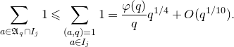 \begin{equation} \sum_{a\in \mathfrak{A}_q\cap I_j}1\leqslant \sum_{\substack{(a, q)=1 \\ a\in I_j}} 1 = \frac{\varphi(q)}{q}q^{1/4}+ O(q^{1/10 }).\end{equation}
Given
 $\varepsilon\in(0, 1)$
, we let
$\varepsilon\in(0, 1)$
, we let
 $E_{\pm}=\{j \mid \pm ( \# I_{j}\cap \mathfrak{A}_q-\varphi(q)q^{-3/4}) > \varepsilon \varphi(q)q^{-3/4}\}$
and
$E_{\pm}=\{j \mid \pm ( \# I_{j}\cap \mathfrak{A}_q-\varphi(q)q^{-3/4}) > \varepsilon \varphi(q)q^{-3/4}\}$
and
 $E=E_{+}\cup E_-$
. By (3.2) it is clear that
$E=E_{+}\cup E_-$
. By (3.2) it is clear that
 $E_+$
is empty if we assume q is large enough. Also, summing (3.2) over
$E_+$
is empty if we assume q is large enough. Also, summing (3.2) over
 $j\notin E_{-}$
, we deduce from Lemma 3.1 that
$j\notin E_{-}$
, we deduce from Lemma 3.1 that
 $\# E=\# E_{-}=O(\varepsilon q^{3/4})$
. Now, for each
$\# E=\# E_{-}=O(\varepsilon q^{3/4})$
. Now, for each
 $j\notin E$
we fix any
$j\notin E$
we fix any
 $y_j\in I_{j}\cap \mathfrak{A}_q$
. Since
$y_j\in I_{j}\cap \mathfrak{A}_q$
. Since
 $\|G\|_\infty, \|G'\|_\infty<\infty$
, by Lemma 3.1 and Equations (3.2) and (3.1), we have
$\|G\|_\infty, \|G'\|_\infty<\infty$
, by Lemma 3.1 and Equations (3.2) and (3.1), we have
 \begin{equation*} \begin{split} \mathcal{R} {}& = \frac1{\varphi(q)} \sum_{a\in \mathfrak{A}_q} G(f^*(a/q)) + o(1) \\ &{}= \frac1{\varphi(q)} \sum_{\substack{0\leqslant j \leqslant q^{3/4}\\ j\notin E}} \sum_{a\in I_j\cap \mathfrak{A}_q} G(f^*(a/q)) + o(1)+O(\varepsilon)\\ &{}= \frac1{\varphi(q)} \sum_{\substack{0\leqslant j \leqslant q^{3/4}\\ j\notin E}} G(f^*(y_j)) \sum_{a\in I_j\cap \mathfrak{A}_q} 1+ o(1)+O(\varepsilon). \end{split}\end{equation*}
For
 $j\notin E$
the inner sum is
$j\notin E$
the inner sum is
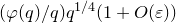 $({\varphi(q)}/{q})q^{1/4}(1+O(\varepsilon))$
and thus by (3.1) and Lemma 3.2 we deduce
$({\varphi(q)}/{q})q^{1/4}(1+O(\varepsilon))$
and thus by (3.1) and Lemma 3.2 we deduce
 \begin{align*} \mathcal{R} {} &{}= \frac1{q^{3/4}} \sum_{\substack{0\leqslant j \leqslant q^{3/4}\\ j\notin E}} G(f^*(y_j)) + o(1)+O(\varepsilon)\\ &{}= \sum_{\substack{0\leqslant j \leqslant q^{3/4}\\ j\notin E}} \int_{(\frac1qI_j)\cap \mathfrak{T}_q}G(f^*(x)) \mathop{}\!{d} x + o(1)+O(\varepsilon)\\ &{}= \int_{ \mathfrak{T}_q}G(f^*(x)) \mathop{}\!{d} x + o(1)+O(\varepsilon)\\ &{}= \int_{ [0,1]}G(f^*(x)) \mathop{}\!{d} x + o(1)+O(\varepsilon),\end{align*}
since
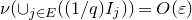 $\nu(\cup_{j\in E}((1/q)I_j))=O(\varepsilon)$
. Letting
$\nu(\cup_{j\in E}((1/q)I_j))=O(\varepsilon)$
. Letting
 $\varepsilon\to0$
sufficiently slowly, we obtain the claimed result.
$\varepsilon\to0$
sufficiently slowly, we obtain the claimed result.
3.2 Proof of Theorem 1.3: Diffuseness when
$\operatorname{Re}(k)<0$

We now focus on the case
 $\operatorname{Re}(k)<0$
and aim to show the second part of Theorem 1.3.
$\operatorname{Re}(k)<0$
and aim to show the second part of Theorem 1.3.
Proposition 3.4. Let k, f,
 $f^\triangleleft$
and h as in Theorem 1.2 and let
$f^\triangleleft$
and h as in Theorem 1.2 and let
 $\phi:\mathbb{C}\to\mathbb{R}$
be a linear form. Assume further that h is real-analytic on
$\phi:\mathbb{C}\to\mathbb{R}$
be a linear form. Assume further that h is real-analytic on
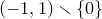 $(-1,1)\smallsetminus\{0\}$
. Assume that for some choice of sign
$(-1,1)\smallsetminus\{0\}$
. Assume that for some choice of sign
 $\pm$
, there exists a set of positive measure
$\pm$
, there exists a set of positive measure
 $C \subseteq {\pm \mathbb{R}_{>0}}$
and a constant
$C \subseteq {\pm \mathbb{R}_{>0}}$
and a constant
 $\alpha \in\mathbb{R}$
such that
$\alpha \in\mathbb{R}$
such that
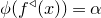 $\phi(f^\triangleleft(x))=\alpha$
for
$\phi(f^\triangleleft(x))=\alpha$
for
 $x\in C$
. Then
$x\in C$
. Then
 $\phi(f^\triangleleft(x))=\alpha$
for almost all
$\phi(f^\triangleleft(x))=\alpha$
for almost all
 $x\in \pm \mathbb{R}_{>0}$
.
$x\in \pm \mathbb{R}_{>0}$
.
This clearly implies the second part of Theorem 1.3 and concludes its proof.
Proof of Proposition 3.4. We start with the case
 $k\in\mathbb{R}$
. Since the real part of a real-analytic function is real-analytic, we have that
$k\in\mathbb{R}$
. Since the real part of a real-analytic function is real-analytic, we have that
 $\phi\circ f$
is a quantum modular form of weight k and real-analytic period function
$\phi\circ f$
is a quantum modular form of weight k and real-analytic period function
 $\phi\circ h$
. In particular, we can assume that f is real valued and that
$\phi\circ h$
. In particular, we can assume that f is real valued and that
 $\phi$
restricted to
$\phi$
restricted to
 $\mathbb{R}$
is the identity function.
$\mathbb{R}$
is the identity function.
By Theorems 1.1 and 1.2, there exists a full measure set X with
 $f^\triangleleft$
well defined on X. Note that Equation (1.2) holds on
$f^\triangleleft$
well defined on X. Note that Equation (1.2) holds on
 $X\smallsetminus\{0\}$
with f replaced by
$X\smallsetminus\{0\}$
with f replaced by
 $f^\triangleleft$
, by taking the limit along convergents and using the definition (1.6). We also recall that in our proof of Theorem 1.2, the set X was taken to be
$f^\triangleleft$
, by taking the limit along convergents and using the definition (1.6). We also recall that in our proof of Theorem 1.2, the set X was taken to be
 $X=\mathfrak{S}$
from Lemma 2.2. It is clear that
$X=\mathfrak{S}$
from Lemma 2.2. It is clear that
 $\mathfrak{S}$
is closed under any fixed inverse branch of the Gauss map. We may thus assume that X has this property.
$\mathfrak{S}$
is closed under any fixed inverse branch of the Gauss map. We may thus assume that X has this property.
We assume
 $C\subseteq \mathbb{R}_{>0}$
, the other case being analogous. Also, by periodicity we can assume
$C\subseteq \mathbb{R}_{>0}$
, the other case being analogous. Also, by periodicity we can assume
 $ C\subseteq [0,1]\cap X$
. For any
$ C\subseteq [0,1]\cap X$
. For any
 $\varepsilon>0$
, by Lebesgue’s density theorem we can find an interval
$\varepsilon>0$
, by Lebesgue’s density theorem we can find an interval
 $I\subseteq (0,1)$
such that
$I\subseteq (0,1)$
such that
 $\nu(C\cap I)\geqslant (1-\varepsilon) \nu(I)$
. It follows that there exists an even
$\nu(C\cap I)\geqslant (1-\varepsilon) \nu(I)$
. It follows that there exists an even
 $g\in\mathbb{N}$
and an inverse branch
$g\in\mathbb{N}$
and an inverse branch
 $U_{\boldsymbol b}$
of
$U_{\boldsymbol b}$
of
 $T^g$
given by
$T^g$
given by
 $U_{\boldsymbol b}(y) = [0; b_1, \dotsc, b_g+ y]$
for some coefficients
$U_{\boldsymbol b}(y) = [0; b_1, \dotsc, b_g+ y]$
for some coefficients
 ${\boldsymbol b} = (b_1, \dotsc, b_g)\in\mathbb{N}^g$
, such that
${\boldsymbol b} = (b_1, \dotsc, b_g)\in\mathbb{N}^g$
, such that
 $D := \{x\in [0,1]\cap X\mid U_{\boldsymbol b}(x)\in C\}$
has measure
$D := \{x\in [0,1]\cap X\mid U_{\boldsymbol b}(x)\in C\}$
has measure
 $1-O(\varepsilon)$
. Repeatedly applying the reciprocity formula to
$1-O(\varepsilon)$
. Repeatedly applying the reciprocity formula to
 $U_{{\boldsymbol b}}(x)$
for any
$U_{{\boldsymbol b}}(x)$
for any
 $x\in D$
, we have
$x\in D$
, we have
 \begin{equation} \alpha= f^\triangleleft( U_{{\boldsymbol b}}(x)) = \sum_{j= 0}^{g-1} \bigg(\prod_{i=0}^{j-1} T^i(U_{{\boldsymbol b}}(x))\bigg)^{\!{-}k} h((-1)^j T^j(U_{{\boldsymbol b}}(x)))+\bigg(\prod_{i=0}^{g-1} T^i(U_{{\boldsymbol b}}(x))\bigg)^{\!{-}k}f^\triangleleft (x). \end{equation}
Note that
 $T^i\circ U_{\boldsymbol b}$
is a smooth map, and in fact a homography, for any
$T^i\circ U_{\boldsymbol b}$
is a smooth map, and in fact a homography, for any
 $i\leqslant g$
. In particular, solving for
$i\leqslant g$
. In particular, solving for
 $f^\triangleleft(x)$
, we obtain that
$f^\triangleleft(x)$
, we obtain that
 $f^\triangleleft$
is given on D by a function which is real-analytic on (0,1). For
$f^\triangleleft$
is given on D by a function which is real-analytic on (0,1). For
 $\varepsilon$
sufficiently small we must have
$\varepsilon$
sufficiently small we must have
 $\nu(C\cap D)\geqslant \nu(C)-\nu([0,1]\smallsetminus D)>0$
, and thus by analytic continuation this implies that
$\nu(C\cap D)\geqslant \nu(C)-\nu([0,1]\smallsetminus D)>0$
, and thus by analytic continuation this implies that
 $f^\triangleleft(x)=\alpha$
for all
$f^\triangleleft(x)=\alpha$
for all
 $x\in D$
. Since
$x\in D$
. Since
 $\varepsilon>0$
is arbitrary, we conclude that
$\varepsilon>0$
is arbitrary, we conclude that
 $f^\triangleleft(x)=\alpha$
for a subset of (0,1) of measure 1.
$f^\triangleleft(x)=\alpha$
for a subset of (0,1) of measure 1.
Now, let us assume
 $k\not\in\mathbb{R}$
and write
$k\not\in\mathbb{R}$
and write
 $k=k_1+ik_2$
with
$k=k_1+ik_2$
with
 $k_i\in\mathbb{R}$
,
$k_i\in\mathbb{R}$
,
 $k_2\neq0$
. We assume
$k_2\neq0$
. We assume
 $\phi(z)=\operatorname{Re}(z)$
, the general case being analogous. We let
$\phi(z)=\operatorname{Re}(z)$
, the general case being analogous. We let
 $\alpha\in\mathbb{R}$
such that
$\alpha\in\mathbb{R}$
such that
 $\operatorname{Re}(f^\triangleleft(x))=\alpha$
for a set
$\operatorname{Re}(f^\triangleleft(x))=\alpha$
for a set
 $C\subseteq[0,1]$
of positive measure. As in the case
$C\subseteq[0,1]$
of positive measure. As in the case
 $k\in\mathbb{R}$
, given
$k\in\mathbb{R}$
, given
 $\varepsilon>0$
we can find
$\varepsilon>0$
we can find
 ${\boldsymbol b}\in\mathbb{N}^g$
such that
${\boldsymbol b}\in\mathbb{N}^g$
such that
 $D:=\{x\in [0,1]\cap X\mid U_{\boldsymbol b}(x)\in C\}$
has measure
$D:=\{x\in [0,1]\cap X\mid U_{\boldsymbol b}(x)\in C\}$
has measure
 $1-O(\varepsilon)$
. Since (0,1] can be written as the disjoint union
$1-O(\varepsilon)$
. Since (0,1] can be written as the disjoint union
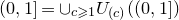 $(0,1]=\cup_{c\geqslant 1}U_{(c)}((0,1])$
, we have
$(0,1]=\cup_{c\geqslant 1}U_{(c)}((0,1])$
, we have
 \begin{align*} \sum_{c\ge1}\nu(\{x\in U_c((0,1])\mid U_{\boldsymbol b}(x)\notin C\})=1-\nu( D)=O(\varepsilon). \end{align*}
In particular,
 $\nu(\{x\in U_c((0,1])\mid U_{\boldsymbol b}(x)\notin C\})=O(\varepsilon)$
for all
$\nu(\{x\in U_c((0,1])\mid U_{\boldsymbol b}(x)\notin C\})=O(\varepsilon)$
for all
 $c\in\mathbb{N}$
and thus also
$c\in\mathbb{N}$
and thus also
 $\nu(\{x\in (0,1]\mid U_{({\boldsymbol b},c)}(x)\notin C\})=O(K^2\varepsilon)$
for all
$\nu(\{x\in (0,1]\mid U_{({\boldsymbol b},c)}(x)\notin C\})=O(K^2\varepsilon)$
for all
 $c\leqslant K$
. Letting
$c\leqslant K$
. Letting
 $D_c := \{x\in [0,1]\cap X\mid U_{({\boldsymbol b},c)}(x)\in C\}$
, we then have
$D_c := \{x\in [0,1]\cap X\mid U_{({\boldsymbol b},c)}(x)\in C\}$
, we then have
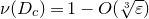 $\nu(D_c)=1-O(\sqrt[3]{\varepsilon})$
for all
$\nu(D_c)=1-O(\sqrt[3]{\varepsilon})$
for all
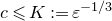 $c\leqslant K:=\varepsilon^{-1/3}$
.
$c\leqslant K:=\varepsilon^{-1/3}$
.
Next, we write the formula (3.3) with
 ${\boldsymbol b}_1=({\boldsymbol b},c_1)$
and
${\boldsymbol b}_1=({\boldsymbol b},c_1)$
and
 ${\boldsymbol b}_2=({\boldsymbol b},c_2)$
in place of
${\boldsymbol b}_2=({\boldsymbol b},c_2)$
in place of
 ${\boldsymbol b}$
for some
${\boldsymbol b}$
for some
 $c_1,c_2\leqslant K$
. Taking the real part of the resulting equations, for
$c_1,c_2\leqslant K$
. Taking the real part of the resulting equations, for
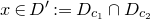 $x \in D':=D_{c_1}\cap D_{c_2}$
we find
$x \in D':=D_{c_1}\cap D_{c_2}$
we find
 \begin{align} \alpha &= A_j(x)+\operatorname{Re} (B_j(x)^{k}f^\triangleleft (x)) ,\quad j=1,2, \end{align}
where for
 $j=1,2$
we have that
$j=1,2$
we have that
 $B_j(x)=(\prod_{i=0}^{g} T^i(U_{({\boldsymbol b},c_j)}(x)))^{-1}$
and
$B_j(x)=(\prod_{i=0}^{g} T^i(U_{({\boldsymbol b},c_j)}(x)))^{-1}$
and
 $A_j$
is real-analytic on (0,1). Notice that
$A_j$
is real-analytic on (0,1). Notice that
 $B_j(x)=v_{g-1}+(c_j+x)v_{g}$
, where
$B_j(x)=v_{g-1}+(c_j+x)v_{g}$
, where
 $v_{g-1}$
and
$v_{g-1}$
and
 $v_g$
are the partial denominators of
$v_g$
are the partial denominators of
 $[0;b_1,\ldots,b_{g-1}]$
and
$[0;b_1,\ldots,b_{g-1}]$
and
 $[0;b_1,\ldots,b_{g}]$
, respectively. In particular, if
$[0;b_1,\ldots,b_{g}]$
, respectively. In particular, if
 $c_1,c_2\in[\sqrt K, K]$
then
$c_1,c_2\in[\sqrt K, K]$
then
 $B_2(x)/B_1(x)={c_2}/{c_1}+O(\sqrt[6]\varepsilon)$
uniformly in
$B_2(x)/B_1(x)={c_2}/{c_1}+O(\sqrt[6]\varepsilon)$
uniformly in
 $x\in[0,1]$
.
$x\in[0,1]$
.
Writing
 $L_j(x):=k_2\log(B_j(x))$
, Equation (3.4) becomes
$L_j(x):=k_2\log(B_j(x))$
, Equation (3.4) becomes
 \begin{align*} \alpha &= A_1(x)+B_j(x)^{k_1}\operatorname{Re}(f^\triangleleft (x))\cos(L_j(x))-B_j(x)^{k_1}\operatorname{Im}(f^\triangleleft (x))\sin(L_j(x))\quad (j\in\{1,2\},\ x\in D'). \end{align*}
This is a system in
 $\operatorname{Re}(f^\triangleleft (x)),\operatorname{Im}(f^\triangleleft (x))$
of determinant
$\operatorname{Re}(f^\triangleleft (x)),\operatorname{Im}(f^\triangleleft (x))$
of determinant
 $B_1(x)^{k_1}B_2(x)^{k_1}\sin(L_1(x)-L_2(x))$
and solving for
$B_1(x)^{k_1}B_2(x)^{k_1}\sin(L_1(x)-L_2(x))$
and solving for
 $\operatorname{Re}(f(x))$
we find
$\operatorname{Re}(f(x))$
we find
 \begin{align} \operatorname{Re}(f^\triangleleft(x))=\frac{(\alpha-A_2(x)) B_1(x)^{k_1} \sin(L_1(x))-(\alpha-A_1(x)) B_2(x)^{k_1} \sin(L_2(x))}{B_1(x)^{k_1}B_2(x)^{k_1}\sin(L_1(x)-L_2(x))} \end{align}
on
 $x\in D'$
. Now, for
$x\in D'$
. Now, for
 $\varepsilon$
sufficiently small, we have
$\varepsilon$
sufficiently small, we have
 \begin{align*} \sin(L_1(x)-L_2(x))=\sin(k_2\log(c_2/c_1)+O(\sqrt[6]\varepsilon)) \end{align*}
uniformly for
 $x\in[0,1]$
. Thus, for
$x\in[0,1]$
. Thus, for
 $\varepsilon$
sufficiently small we can find
$\varepsilon$
sufficiently small we can find
 $c_1,c_2\in \mathbb{N}\cap [\sqrt K,K]$
such that
$c_1,c_2\in \mathbb{N}\cap [\sqrt K,K]$
such that
 $\sin(L_1(x)-L_2(x))$
does not vanish on
$\sin(L_1(x)-L_2(x))$
does not vanish on
 $(0,1).$
For this choice one has that the right-hand side of (3.5) is analytic on (0,1). Since
$(0,1).$
For this choice one has that the right-hand side of (3.5) is analytic on (0,1). Since
 $\nu(D')=1-O(\sqrt[3]\varepsilon)$
, we then reach the conclusion as in the case
$\nu(D')=1-O(\sqrt[3]\varepsilon)$
, we then reach the conclusion as in the case
 $k\in\mathbb{R}$
.
$k\in\mathbb{R}$
.
3.3 The continuity of the cumulative distribution function when
$\operatorname{Re}(k)>0$

We prove the following generalization of Theorem 1.7. Also, as in § 2.4.1, we allow for a twist by a root of unity
 $\vartheta$
and assume f satisfies (2.26).
$\vartheta$
and assume f satisfies (2.26).
Theorem 3.5. Let
 $\phi:\mathbb{C}\to\mathbb{R}$
be a linear form,
$\phi:\mathbb{C}\to\mathbb{R}$
be a linear form,
 $\operatorname{Re}(k)>0$
, and let
$\operatorname{Re}(k)>0$
, and let
 $h:\mathbb{R}\smallsetminus\{0\}\to\mathbb{R}$
be a function satisfying either of the following two conditions.
$h:\mathbb{R}\smallsetminus\{0\}\to\mathbb{R}$
be a function satisfying either of the following two conditions.
-
(1*) The function h extends to a continuous function on
$[-1,1]$
, and either
$\operatorname{Im} k = 0$
and there exists
$p\in\mathbb{Z}$
,
$\alpha\in(-1, 1)$
such that
$\phi(\vartheta^p h(\alpha)) \neq 0$
; or
$\operatorname{Im} k \neq 0$
and there exists
$\alpha\in(-1, 1)$
such that
$h(\alpha)\neq 0$
. -
(2*) One has
$\lim_{x\to 0^\pm}|h(x)|=\infty$
for a choice of
$\pm$
, there exists
$\delta\in(0,1)$
such that
$h(x)\ll {e}^{|x|^{-1+\delta}}$
for
$|x|\leqslant1$
and-
– either
$\operatorname{Im}(k)=0$
and there exists
$p\in\mathbb{Z}$
such that for all small
$\varepsilon>0$
, (3.6)
\begin{equation} \liminf_{x\to 0^\pm} \inf\bigg\{\bigg|\phi\bigg(\vartheta^p \frac{h(x)-{u} ^k h({u} x)}{|h(x)|} \bigg)\bigg|: {| {\log {u}} |} \in (\varepsilon, \varepsilon^{2/3})\bigg\} > 0; \end{equation}
-
– or
$\operatorname{Im}(k)\neq0$
and there exists
${\beta}\in\mathbb{R}$
such that for all small
$\varepsilon>0$
, (3.7)
\begin{equation} \liminf_{x\to 0^\pm} \inf\bigg\{\bigg|\phi\bigg({e}(\alpha) \frac{ h(x)- {u}^{k} h({u} x)}{|h(x)|} \bigg)\bigg|: |\log {u}| \in (\varepsilon, \varepsilon^{2/3}), |\alpha-{\beta}| < \varepsilon^{2/3} \bigg\} > 0. \end{equation}
-


Then the CDF of
 $(\phi\circ f^\triangleright)_\ast( \nu)$
is continuous.
$(\phi\circ f^\triangleright)_\ast( \nu)$
is continuous.
Remark 3.6.
-
– The hypotheses could be relaxed somehow. For instance, instead of (1*), it suffices to ask that h has finite left and right limits at certain rationals along with a non-vanishing condition. This will be clear from our arguments. One could also deal with some cases when the limits (3.6) and (3.7) are zero, as long as one can control the asymptotic of these quantities as
$x\to 0$
. We refer to Remark 3.15 below, as well as to the proof of Corollary 1.14 when
$a=0$
for an example where this consideration is relevant. -
– When h is continuous on
$[-1, 1]$
, the condition (1*) is clearly necessary, since otherwise
$\phi \circ f^\triangleright$
vanishes identically on [0, 1]. -
– Some condition of the type (2*) is necessary in order to prevent examples such as
$h(x) = 1 - {| {x} |}^{-k}$
, for which the function f is constant.


Proof of the second part of Theorem 1.7. Assume first that h is continuous on
 $[-1, 1]$
and non-zero. Then the hypothesis (1*) is clearly satisfied with either
$[-1, 1]$
and non-zero. Then the hypothesis (1*) is clearly satisfied with either
 $\phi=\operatorname{Re}$
or
$\phi=\operatorname{Re}$
or
 $\phi=\operatorname{Im}$
. We deduce that
$\phi=\operatorname{Im}$
. We deduce that
 $(\phi \circ f^\triangleright)_\ast(\nu)$
is diffuse, and therefore so is
$(\phi \circ f^\triangleright)_\ast(\nu)$
is diffuse, and therefore so is
 $f^\triangleright_\ast(\nu)$
.
$f^\triangleright_\ast(\nu)$
.
Assume next that
 $h(x)\ll{e}^{{| {x} |}^{-1+\delta}}$
on
$h(x)\ll{e}^{{| {x} |}^{-1+\delta}}$
on
 $[-1, 1]\smallsetminus\{0\}$
and
$[-1, 1]\smallsetminus\{0\}$
and
 $h(x) \sim c x^{-\lambda}$
as
$h(x) \sim c x^{-\lambda}$
as
 $x\to 0^+$
. Then for
$x\to 0^+$
. Then for
 ${| {\log {u}} |} \leqslant 1$
, we deduce that as
${| {\log {u}} |} \leqslant 1$
, we deduce that as
 $x\to0^+$
,
$x\to0^+$
,
 $$ \frac{h(x) - {u}^k h({u} x)}{{| {h(x)} |}} = \frac{c}{{| {c} |}} (1+o(1)) (1 - {u}^{k-\lambda}) \gg_{\varepsilon,k,\lambda} 1 $$
if additionally
 ${| {\log {u}} |} \geqslant \varepsilon$
. Similarly as above, we deduce that hypothesis (2*) holds for
${| {\log {u}} |} \geqslant \varepsilon$
. Similarly as above, we deduce that hypothesis (2*) holds for
 $\phi=\operatorname{Re}$
or
$\phi=\operatorname{Re}$
or
 $\phi=\operatorname{Im}$
and we deduce that
$\phi=\operatorname{Im}$
and we deduce that
 $f^\triangleright_\ast(\nu)$
is diffuse.
$f^\triangleright_\ast(\nu)$
is diffuse.
This shows that the second part of Theorem 1.7 holds, and concludes its proof.
Remark 3.7. When
 $h(x) = c x^{-\lambda}$
with
$h(x) = c x^{-\lambda}$
with
 $\lambda$
satisfying
$\lambda$
satisfying
 $\operatorname{Re}(k)>0$
but
$\operatorname{Re}(k)>0$
but
 $\lambda\not\in\mathbb{R}$
, hypothesis (2*) no longer holds, but it is plausible that our arguments could be adapted by further localizing the values of x involved in (3.6) and (3.7). We do not pursue this here.
$\lambda\not\in\mathbb{R}$
, hypothesis (2*) no longer holds, but it is plausible that our arguments could be adapted by further localizing the values of x involved in (3.6) and (3.7). We do not pursue this here.
We first give the following lemma.
Lemma 3.8. Let
 $F:[0, 1]\to \mathbb{R}$
be measurable. Assume that for each
$F:[0, 1]\to \mathbb{R}$
be measurable. Assume that for each
 $\varepsilon>0$
, we can find a countable collection
$\varepsilon>0$
, we can find a countable collection
 $(S_j)_j$
of disjoint measurable subsets of [0, 1], such that
$(S_j)_j$
of disjoint measurable subsets of [0, 1], such that
 $$ \sum_j \nu(S_j) \geqslant 1 - \varepsilon, $$
and for each j and
 $y\in S_j$
,
$y\in S_j$
,
 \begin{equation} \nu(\{x \in S_j, F(x)=F(y)\}) \leqslant \varepsilon \nu(S_j). \end{equation}
Then
 $F_*(\nu)$
is continuous.
$F_*(\nu)$
is continuous.
Proof. Let
 $a\in\mathbb{R}$
, and
$a\in\mathbb{R}$
, and
 $X=F^{-1}(\{a\})$
. Let
$X=F^{-1}(\{a\})$
. Let
 $\varepsilon>0$
be arbitrary, and
$\varepsilon>0$
be arbitrary, and
 $(S_j)_j$
given by the hypothesis. For each j, either
$(S_j)_j$
given by the hypothesis. For each j, either
 $S_j\cap X$
is empty, or there exists
$S_j\cap X$
is empty, or there exists
 $y\in S_j$
such that
$y\in S_j$
such that
 $F(y)=a$
and then
$F(y)=a$
and then
 $$ \nu(X\cap S_j) = \nu(\{x \in S_j, F(x) = F(y)\}) \leqslant \varepsilon \nu(S_j) $$
by hypothesis. In both cases we have
 $\nu(X \cap S_j) \leqslant \varepsilon \nu(S_j)$
. Summing over j, we find
$\nu(X \cap S_j) \leqslant \varepsilon \nu(S_j)$
. Summing over j, we find
 $$ \nu(X) \leqslant \nu([0, 1]\smallsetminus \cup_j S_j) + \sum_j \nu(X \cap S_j) \leqslant 2\varepsilon, $$
and letting
 $\varepsilon\to0$
gives the conclusion.
$\varepsilon\to0$
gives the conclusion.
We divide the proof depending on whether (1*) or (2*) holds.
3.3.1 The case of bounded h.
Let
 $N\in\mathbb{Z}_{>0}$
be the order of
$N\in\mathbb{Z}_{>0}$
be the order of
 $\vartheta$
as a root of unity, so that
$\vartheta$
as a root of unity, so that
 $$ \vartheta^N = 1, $$
where
 $\vartheta$
is the automorphy factor in the generalized period relation (2.26). We recall that
$\vartheta$
is the automorphy factor in the generalized period relation (2.26). We recall that
 $\vartheta_j$
was defined in (2.27). Recall also from (2.31) that the notation
$\vartheta_j$
was defined in (2.27). Recall also from (2.31) that the notation
 $\vartheta_j(x)$
for a number
$\vartheta_j(x)$
for a number
 $x\in\mathbb{Q}$
depends on how we expand x in CF when x is rational. In what follows, we will work with the expansion of odd length. For each
$x\in\mathbb{Q}$
depends on how we expand x in CF when x is rational. In what follows, we will work with the expansion of odd length. For each
 $g\geqslant 1$
, we define
$g\geqslant 1$
, we define
 $e_g(x) \in \mathbb{Z}/N\mathbb{Z}$
through
$e_g(x) \in \mathbb{Z}/N\mathbb{Z}$
through
 $ \vartheta_g(x) = \vartheta^{e_g(x)}$
and notice that by definition we have
$ \vartheta_g(x) = \vartheta^{e_g(x)}$
and notice that by definition we have
 \begin{equation} e_g(x)\equiv e_{g-1}(x)+(-1)^g b_g+3(-1)^{g+1}\pmod{N}.\end{equation}
Given
 $c_1, \dotsc, c_\ell\geqslant 1$
, we denote
$c_1, \dotsc, c_\ell\geqslant 1$
, we denote
 \begin{equation} \begin{split} J(c_1, \dotsc, c_\ell) := {}& \{x\in[0, 1], b_i(x) = c_i \text{ for } 1\leqslant i \leqslant \ell \}, \\ \mu(c_1, \dotsc, c_\ell) := {}& \nu(J(c_1, \dotsc, c_\ell)). \end{split}\end{equation}
By [Reference KhintchineKhi63, p. 57], we have
 \begin{equation} \mu(c_1, \dotsc, c_\ell) = \frac1{v_\ell(x)(v_\ell(x) + v_{\ell-1}(x))} \asymp \frac1{v_\ell(x)^2} \quad (x = [0; c_1, \dotsc, c_\ell]).\end{equation}
Lemma 3.9. Let
 $m\in \mathbb{N}$
,
$m\in \mathbb{N}$
,
 $K>1$
and
$K>1$
and
 $(L_1,\ldots,L_m)\in\mathbb{N}^m$
be fixed. Let
$(L_1,\ldots,L_m)\in\mathbb{N}^m$
be fixed. Let
 $V\geqslant1$
, and for each
$V\geqslant1$
, and for each
 $e\in\mathbb{Z}/N\mathbb{Z}$
and
$e\in\mathbb{Z}/N\mathbb{Z}$
and
 $\omega>0$
, let
$\omega>0$
, let
 $\mathscr{B}(e, \omega) \subset \mathbb{Z}\cap[\sqrt{V}, K\sqrt{V}]$
be given, and
$\mathscr{B}(e, \omega) \subset \mathbb{Z}\cap[\sqrt{V}, K\sqrt{V}]$
be given, and
 $$ T := \inf_{e\in\mathbb{Z}/N\mathbb{Z},\, \omega>0} \# \mathscr{B}(e, \omega). $$
Also, for
 $x\in(0, 1)\smallsetminus\mathbb{Q}$
, let
$x\in(0, 1)\smallsetminus\mathbb{Q}$
, let
 $$ G_V(x):=\{g\in [V,2 V] \mid b_g(x) \in \mathscr{B}(e_{g-1}(x), v_{g-1}(x)),\, b_{g+i}(x) =L_i\ \forall i=1,\ldots,m\} $$
and let
 $X_{V, \mathscr{B}} = X_{V,\mathscr{B}}(K, L_1, \dotsc, L_m)$
be the subset of
$X_{V, \mathscr{B}} = X_{V,\mathscr{B}}(K, L_1, \dotsc, L_m)$
be the subset of
 $[0,1]\smallsetminus\mathbb{Q}$
such that
$[0,1]\smallsetminus\mathbb{Q}$
such that
 $G_V(x)$
contains at least an even and an odd integer. Then
$G_V(x)$
contains at least an even and an odd integer. Then
 $\nu(X_{V,\mathscr{B}})=1+o(1)$
as
$\nu(X_{V,\mathscr{B}})=1+o(1)$
as
 $V, T \to \infty$
, where the rate of decay of o(1) depends at most on
$V, T \to \infty$
, where the rate of decay of o(1) depends at most on
 $K, L_1, \dotsc, L_m$
.
$K, L_1, \dotsc, L_m$
.
Proof. We show that
 $G_V(x)$
contains an even integer for x in a set of measure
$G_V(x)$
contains an even integer for x in a set of measure
 $1+o(1)$
, the odd integer case being analogous.
$1+o(1)$
, the odd integer case being analogous.
By [Reference KhintchineKhi63, Equation (57)] we have uniformly for
 $\ell\geqslant 1$
and
$\ell\geqslant 1$
and
 $c_1, \dotsc, c_{\ell+1}\geqslant 1$
,
$c_1, \dotsc, c_{\ell+1}\geqslant 1$
,
 \begin{align} \tfrac13 c_{\ell+1}^{-2}\mu(c_1,\ldots,c_{\ell})\leqslant \mu(c_1,\ldots,c_{\ell+1})\leqslant 2 c_{\ell+1}^{-2}\mu(c_1,\ldots,c_{\ell}). \end{align}
In particular, writing
 $L:=\max(L_1,\ldots, L_m)$
, we have for any
$L:=\max(L_1,\ldots, L_m)$
, we have for any
 $c\in\mathbb{Z}_{>0}$
,
$c\in\mathbb{Z}_{>0}$
,
 $$ \mu(c_1,\ldots,c_\ell,c,L_1,\ldots,L_m)\geqslant 3^{-m-1} c^{-2}L^{-2m}\mu(c_1,\ldots,c_{\ell}).$$
Since
 $\sum_{c\in\mathscr{B}(e_\ell, v_\ell)}c^{-2}\geqslant (1/{K^2V})\#{\mathscr{B}(e_\ell, v_\ell)}$
, where
$\sum_{c\in\mathscr{B}(e_\ell, v_\ell)}c^{-2}\geqslant (1/{K^2V})\#{\mathscr{B}(e_\ell, v_\ell)}$
, where
 $e_\ell = e_\ell([0;c_1, \dotsc, c_\ell])$
, it then follows that the measure of
$e_\ell = e_\ell([0;c_1, \dotsc, c_\ell])$
, it then follows that the measure of
 $x\in [0,1]\smallsetminus\mathbb{Q}$
such that none of the integers
$x\in [0,1]\smallsetminus\mathbb{Q}$
such that none of the integers
 $g\in\{2{\lfloor {V/2} \rfloor} + \ell (2m+2) \mid 1\leqslant \ell \leqslant V /(2m+2)\}$
satisfy
$g\in\{2{\lfloor {V/2} \rfloor} + \ell (2m+2) \mid 1\leqslant \ell \leqslant V /(2m+2)\}$
satisfy
 $b_g(x) \in \mathscr{B}$
is
$b_g(x) \in \mathscr{B}$
is
 $$ \ll (1- K^{-2}(3L)^{-3m}TV^{-1})^{{\lfloor {V/(2m+2)} \rfloor}} = o(1) $$
as
 $V, T\to\infty$
with m, L fixed. The lemma then follows.
$V, T\to\infty$
with m, L fixed. The lemma then follows.
We now prove Theorem 3.5. To illustrate Remark 3.6, we assume only that h is bounded on
 $[-1, 1]$
, not necessarily continuous, and that it has finite left or right limit at 0. We assume it is the former, the latter case being analogous, as we will comment after the proof. If
$[-1, 1]$
, not necessarily continuous, and that it has finite left or right limit at 0. We assume it is the former, the latter case being analogous, as we will comment after the proof. If
 $\operatorname{Im}(k)=0$
, we suppose that
$\operatorname{Im}(k)=0$
, we suppose that
 $\phi(\vartheta^p h(0^-))\neq0$
for some
$\phi(\vartheta^p h(0^-))\neq0$
for some
 $p\in\mathbb{Z}$
, whereas if
$p\in\mathbb{Z}$
, whereas if
 $\operatorname{Im}(k)\neq0$
, we assume that
$\operatorname{Im}(k)\neq0$
, we assume that
 $h(0^-)\neq0$
and set
$h(0^-)\neq0$
and set
 $p:=0$
. Moreover, we let
$p:=0$
. Moreover, we let
 \begin{equation} \kappa\in\mathbb{R}, \quad \phi({e}(-\kappa) \vartheta^p h(0^-)) \text{ is maximal.}\end{equation}
This means, in other terms, that for any
 $z\in\mathbb{C}$
,
$z\in\mathbb{C}$
,
 \begin{equation} \phi(\vartheta^p h(0^-) z) = {| {h(0^-)} |} \operatorname{Re}(e(\kappa) z).\end{equation}
If
 $\operatorname{Im}(k)=0$
, then setting
$\operatorname{Im}(k)=0$
, then setting
 $z=1$
we see that
$z=1$
we see that
 $\kappa\not\equiv\pm\frac12\ (\textrm{mod}\,1)$
by hypothesis.
$\kappa\not\equiv\pm\frac12\ (\textrm{mod}\,1)$
by hypothesis.
We define our choice of sets
 $\mathscr{B} = \mathscr{B}(e, \omega)$
. We let
$\mathscr{B} = \mathscr{B}(e, \omega)$
. We let
 $\xi\in(0,1)$
be a parameter, on which these sets will depend. For
$\xi\in(0,1)$
be a parameter, on which these sets will depend. For
 $e\in\mathbb{Z}/N\mathbb{Z}$
,
$e\in\mathbb{Z}/N\mathbb{Z}$
,
 $\omega>0$
, let
$\omega>0$
, let
 $K=2$
if
$K=2$
if
 $\operatorname{Im}(k)=0$
and
$\operatorname{Im}(k)=0$
and
 $K=\max(2,e^{3\pi/{| {\operatorname{Im}(k)} |}})$
otherwise. Also, let
$K=\max(2,e^{3\pi/{| {\operatorname{Im}(k)} |}})$
otherwise. Also, let
 $ \mathscr{B}(e, \omega) = \mathscr{B}_{V, \xi, N, k}(e, \omega)$
be defined by
$ \mathscr{B}(e, \omega) = \mathscr{B}_{V, \xi, N, k}(e, \omega)$
be defined by
 \begin{equation} \begin{aligned} \mathscr{B}(e, \omega) := {}& \Bigg\{b\in\mathbb{Z}\cap [\sqrt V, K\sqrt V] \colon b\equiv 3 - (p+e)\pmod{N} \\ & \quad \text{and }\left. \begin{cases} -\xi \leqslant \bigg\{\dfrac{\operatorname{Im} (k)}{2\pi}\log (\omega\sqrt V)-\kappa\bigg\} + \dfrac{\operatorname{Im} (k)}{2\pi}\log (b/\sqrt V) \leqslant \xi & \text{if } k\notin\mathbb{R} \\[2pt] 0 \leqslant \log (b/\sqrt V) \leqslant \xi & \text{if } k\in\mathbb{R} \end{cases}\right\}, \end{aligned}\end{equation}
where
 $\{\cdot\}$
denotes the fractional part, and
$\{\cdot\}$
denotes the fractional part, and
 $\kappa$
was defined at (3.13). Here our choice of K ensures that the set
$\kappa$
was defined at (3.13). Here our choice of K ensures that the set
 $\mathscr{B}$
is not void for V large enough, and in fact
$\mathscr{B}$
is not void for V large enough, and in fact
 \begin{equation} \#\mathscr{B} \gg_{k, N} \xi \sqrt{V}\end{equation}
for V large enough in terms of k, N and
 $\xi$
. Moreover, on the one hand, by (3.9) the congruence condition ensures that whenever a number
$\xi$
. Moreover, on the one hand, by (3.9) the congruence condition ensures that whenever a number
 $x\in[0,1]\smallsetminus\mathbb{Q}$
satisfies
$x\in[0,1]\smallsetminus\mathbb{Q}$
satisfies
 $b_g(x) \in \mathscr{B}(e_{g-1}(x), v_{g-1}(x))$
with g even, we have
$b_g(x) \in \mathscr{B}(e_{g-1}(x), v_{g-1}(x))$
with g even, we have
 $e_g(x) \equiv -p\ (\textrm{mod}\,N)$
, and therefore we deduce
$e_g(x) \equiv -p\ (\textrm{mod}\,N)$
, and therefore we deduce
 \begin{equation} \vartheta_g(x) = \vartheta^{-p} \quad (g\in G_V(x)\cap 2\mathbb{Z}).\end{equation}
On the other hand, the condition involving
 $\|\cdot\|_{\mathbb{R}/\mathbb{Z}}$
ensures that
$\|\cdot\|_{\mathbb{R}/\mathbb{Z}}$
ensures that
 \begin{equation} \operatorname{Re}({e}(\kappa) (v_{g-1}(x) b_g(x))^{-i\operatorname{Im} k}) = 1 + O(\xi^2) \quad (\operatorname{Im} k \neq 0, g\in G_V(x)) \end{equation}
by the Taylor expansion of the cosine, with an absolute implicit constant.
We let
 $L_1,\ldots,L_m\in\mathbb{N}$
be chosen later and take
$L_1,\ldots,L_m\in\mathbb{N}$
be chosen later and take
 $X_{V,\mathscr{B}}$
,
$X_{V,\mathscr{B}}$
,
 $G_V(x)$
as in Lemma 3.9. For all even g and all
$G_V(x)$
as in Lemma 3.9. For all even g and all
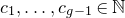 $c_1, \dotsc, c_{g-1}\in \mathbb{N}$
, we let
$c_1, \dotsc, c_{g-1}\in \mathbb{N}$
, we let
 \begin{equation} S_{g, (c_i), \mathscr{B}} := \{x \in (0,1)\smallsetminus\mathbb{Q}: \forall i<g, b_i(x) = c_i; g\in G_V(x)\cap2\mathbb{Z}; \forall j\geqslant 1, g-2j \not\in G_V(x)\},\end{equation}
that is,
 $S_{g, (c_i), \mathscr{B}}$
is the subset of
$S_{g, (c_i), \mathscr{B}}$
is the subset of
 $ J(c_1,\ldots,c_{g-1})$
such that g is the smallest even element of
$ J(c_1,\ldots,c_{g-1})$
such that g is the smallest even element of
 $G_V(x)$
. We will drop the subscript
$G_V(x)$
. We will drop the subscript
 $\mathscr{B}$
from the notation.
$\mathscr{B}$
from the notation.
Lemma 3.10. Assume that
 $L_i < \sqrt{V}$
for all
$L_i < \sqrt{V}$
for all
 $1\leqslant i \leqslant m$
and that
$1\leqslant i \leqslant m$
and that
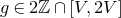 $g\in2\mathbb{Z}\cap[V,2V]$
. For all
$g\in2\mathbb{Z}\cap[V,2V]$
. For all
 $c_1, \dotsc, c_{g-1},c \geqslant 1$
and
$c_1, \dotsc, c_{g-1},c \geqslant 1$
and
 $\varepsilon>0$
, we have
$\varepsilon>0$
, we have
 $$ \nu(\{ x\in S_{g, (c_i)} \colon {| {b_g(x) - c} |} \leqslant \varepsilon \sqrt{V} \}) \ll \varepsilon \xi^{-1} \nu(S_{g, (c_i)}) $$
where the constant depends on m, k and N at most.
Proof. We start by observing that the condition
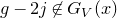 $g-2j \not\in G_V(x)$
in the definition of
$g-2j \not\in G_V(x)$
in the definition of
 $S_{g, (c_i), \mathscr{B}}$
reduces to a condition on the first
$S_{g, (c_i), \mathscr{B}}$
reduces to a condition on the first
 $g-1$
partial quotients of x,
$g-1$
partial quotients of x,
 $c_1,\ldots, c_{g-1}$
, if
$c_1,\ldots, c_{g-1}$
, if
 $j>m/2$
. In particular, we can assume this condition is satisfied, since otherwise
$j>m/2$
. In particular, we can assume this condition is satisfied, since otherwise
 $S_{g, (c_i)} = \emptyset$
and the result is trivial. Similarly, we can assume
$S_{g, (c_i)} = \emptyset$
and the result is trivial. Similarly, we can assume
 $c\in [(1-\varepsilon)\sqrt V,(K+\varepsilon)\sqrt V]$
.
$c\in [(1-\varepsilon)\sqrt V,(K+\varepsilon)\sqrt V]$
.
Next, we observe that if
 $1\leqslant j<m/2$
, then the condition
$1\leqslant j<m/2$
, then the condition
 $g-2j \not\in G_V(x)$
follows from the truth of the other conditions in the definition of
$g-2j \not\in G_V(x)$
follows from the truth of the other conditions in the definition of
 $S_{g, (c_i)}$
. Indeed, for
$S_{g, (c_i)}$
. Indeed, for
 $g\in G_V(x)$
we have
$g\in G_V(x)$
we have
 $b_g(x)\in\mathscr{B}$
and
$b_g(x)\in\mathscr{B}$
and
 $b_{g+i}(x) = L_i$
for
$b_{g+i}(x) = L_i$
for
 $1\leqslant i \leqslant m$
, so that
$1\leqslant i \leqslant m$
, so that
 $b_{g-2j+2j}(x)=b_g(x) \geqslant \sqrt{V} > L_{2j}$
and thus
$b_{g-2j+2j}(x)=b_g(x) \geqslant \sqrt{V} > L_{2j}$
and thus
 $g-2j\notin G_V(x)$
. Recalling the notation (3.10), we thus have
$g-2j\notin G_V(x)$
. Recalling the notation (3.10), we thus have
 $$ \{x\in S_{g, (c_i)} \colon b_g(x)=c'\}= J(c_1,\ldots,c_{g-1},c',L_1,\ldots,L_m) $$
for all
 $c' \in \mathscr{B}(e_{g-1}(x'), v_{g-1}(x'))$
with
$c' \in \mathscr{B}(e_{g-1}(x'), v_{g-1}(x'))$
with
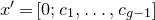 $x'=[0;c_1,\ldots, c_{g-1}]$
. By (3.11), for all
$x'=[0;c_1,\ldots, c_{g-1}]$
. By (3.11), for all
 $c' \in[(1-\varepsilon)\sqrt V, (K+\varepsilon)\sqrt V]$
, we have
$c' \in[(1-\varepsilon)\sqrt V, (K+\varepsilon)\sqrt V]$
, we have
 $$ \mu(0; c_1, \dotsc, c_{g-1}, c', L_1, \dotsc, L_m) \asymp \mu(0; c_1, \dotsc, c_{g-1}, c, L_1, \dotsc, L_m) $$
with a constant depending at most on m and K. Then, using (3.16) we deduce on the one hand
 $$ \nu(S_{g, (c_i)}) \gg \xi \sqrt{V} \mu([0; c_1, \dotsc, c_{g-1}, c, L_1, \dotsc, L_m]) $$
and on the other hand
 $$ \nu(\{ x\in S_{g, (c_i)}, {| {b_g(x) - c} |} \leqslant \varepsilon \sqrt{V}\}) \ll \varepsilon \sqrt{V} \mu([0; c_1, \dotsc, c_{g-1}, c, L_1, \dotsc, L_m]). $$
Grouping these two bounds yields our claim.
Let
 $\varepsilon\in(0,1)$
be fixed. We set
$\varepsilon\in(0,1)$
be fixed. We set
 $m=1$
and
$m=1$
and
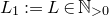 $L_1:=L\in\mathbb{N}_{>0}$
be a parameter. We let
$L_1:=L\in\mathbb{N}_{>0}$
be a parameter. We let
 $X_{V,\mathscr{B}}$
as in Lemma 3.9 and assume that
$X_{V,\mathscr{B}}$
as in Lemma 3.9 and assume that
 $L \to \infty$
as
$L \to \infty$
as
 $V\to\infty$
sufficiently slowly with respect to V, so that we still have
$V\to\infty$
sufficiently slowly with respect to V, so that we still have
 $\nu(X_{V,\mathscr{B}})\to1$
as well as
$\nu(X_{V,\mathscr{B}})\to1$
as well as
 $L<\sqrt V$
. In particular, assuming
$L<\sqrt V$
. In particular, assuming
 $V\geqslant 1$
is large enough, we have
$V\geqslant 1$
is large enough, we have
 \begin{equation*} \nu(X_{V,\mathscr{B}}) \geqslant 1-\varepsilon.\end{equation*}
For
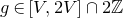 $g\in [V, 2V]\cap 2\mathbb{Z}$
and
$g\in [V, 2V]\cap 2\mathbb{Z}$
and
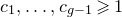 $c_1, \dotsc, c_{g-1}\geqslant 1$
, the sets
$c_1, \dotsc, c_{g-1}\geqslant 1$
, the sets
 $(S_{g, (c_i)})$
are disjoint and, by construction, their union over all g and
$(S_{g, (c_i)})$
are disjoint and, by construction, their union over all g and
 $(c_i)$
contains
$(c_i)$
contains
 $X_{V,\mathscr{B}}$
and thus has measure
$X_{V,\mathscr{B}}$
and thus has measure
 $\geqslant1-\varepsilon$
. The collection of sets
$\geqslant1-\varepsilon$
. The collection of sets
 $(S_{g, (c_i)})$
will play the rôle of
$(S_{g, (c_i)})$
will play the rôle of
 $(S_j)$
in Lemma 3.8.
$(S_j)$
in Lemma 3.8.
Recall that, since h is assumed to be bounded, we have the expression (2.33). Consider one of the sets
 $S_{g, (c_j)}$
, and
$S_{g, (c_j)}$
, and
 $x, y\in S_{g, (c_j)}$
satisfying
$x, y\in S_{g, (c_j)}$
satisfying
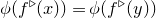 $\phi(f^\triangleright(x))= \phi(f^\triangleright(y))$
. Since the terms
$\phi(f^\triangleright(x))= \phi(f^\triangleright(y))$
. Since the terms
 $j<g$
in (2.33) depend only on
$j<g$
in (2.33) depend only on
 $c_1, \dotsc, c_{g-1}$
, we have
$c_1, \dotsc, c_{g-1}$
, we have
 $f^\triangleright(x) - f^\triangleright(y) = F_g(x) - F_g(y)$
, where
$f^\triangleright(x) - f^\triangleright(y) = F_g(x) - F_g(y)$
, where
 \begin{equation} F_g(x) = \sum_{j=g}^\infty \vartheta_j^{-1}(x) v_j(x)^{-k} h\bigg((-1)^{j-1}\frac{v_{j-1}(x)}{v_j(x)}\bigg) \end{equation}
and similarly for y. If
 $x \in S_{g, (c_j)}$
we have
$x \in S_{g, (c_j)}$
we have
 $v_{g+j}(x)\gg v_{g}(x) L\, \varpi^j$
for
$v_{g+j}(x)\gg v_{g}(x) L\, \varpi^j$
for
 $j\geqslant1$
, whence since g is even and h is bounded, we have
$j\geqslant1$
, whence since g is even and h is bounded, we have
 \begin{align*} F_g(x) & {}=\frac{\vartheta_g(x)^{-1}+o(1)}{v_g(x)^{k}}h(0^-) +O\bigg(\frac{L^{-\operatorname{Re}(k)}}{ v_g(x)^{\operatorname{Re}(k)}}\sum_{j\geqslant1}\frac {\|h\|_\infty}{\varpi^{\operatorname{Re}(k)j}}\bigg)\\ &{} =\frac{\vartheta_g(x)^{-1}+o(1)}{v_g(x)^{k}}h(0^-),\end{align*}
as
 $V \to \infty$
.
$V \to \infty$
.
Consider first the case
 $\operatorname{Im} k = 0$
. By (3.17), we have
$\operatorname{Im} k = 0$
. By (3.17), we have
 \begin{equation} \vartheta_g(x) = \vartheta_g(y) = \vartheta^{-p}.\end{equation}
Also, since
 $b_j(x)=b_j(y)$
for
$b_j(x)=b_j(y)$
for
 $j<g$
and
$j<g$
and
 $b_g(x)\asymp b_g(y)\asymp\sqrt V$
, we have
$b_g(x)\asymp b_g(y)\asymp\sqrt V$
, we have
 $v_{g-1}(x)\asymp v_{g-1}(y)$
and
$v_{g-1}(x)\asymp v_{g-1}(y)$
and
 $v_{g}(x)\asymp v_{g}(y)$
with constants depending only on k. Thus, by (3.14) and the mean value theorem, we deduce that for
$v_{g}(x)\asymp v_{g}(y)$
with constants depending only on k. Thus, by (3.14) and the mean value theorem, we deduce that for
 $\operatorname{Im} k = 0$
we have
$\operatorname{Im} k = 0$
we have
 \begin{align*} 0 = {| {\phi(F_g(x) - F_g(y))} |} {}&= |h(0^-)\cos(2\pi \kappa)||v_g(x)^{-k} - v_g(y)^{-k}| + o(v_g(x)^{-\operatorname{Re} k}) \\{}& \gg |h(0^-)\cos(2\pi \kappa)|\frac{|v_g(x) - v_g(y)|}{v_g(x)^{k+1}}+ o(v_g(x)^{-\operatorname{Re} k}) \\{}& \gg |h(0^-)\cos(2\pi \kappa)|\frac{{| {b_g(x) - b_g(y)} |} V^{-1/2} + o(1)}{v_g(x)^{ k}}.\end{align*}
We deduce that
 ${| {b_g(x) - b_g(y)} |} = o(\sqrt{V})$
as
${| {b_g(x) - b_g(y)} |} = o(\sqrt{V})$
as
 $V\to \infty$
.
$V\to \infty$
.
We reach a similar conclusion when
 $\operatorname{Im} k \neq 0$
. Indeed, in this case we still have (3.22), with
$\operatorname{Im} k \neq 0$
. Indeed, in this case we still have (3.22), with
 $p=0$
. Furthermore, since
$p=0$
. Furthermore, since
 $v_g(x) = v_{g-1} b_g(x) + v_{g-2}(x)$
, we have
$v_g(x) = v_{g-1} b_g(x) + v_{g-2}(x)$
, we have
 $$ \phi(h(0^-) v_g(x)^{-i \operatorname{Im} k}) = {| {h(0^-)} |} \operatorname{Re}({e}(\kappa) (v_{g-1}b_g(x))^{-i\operatorname{Im} k} )(1 + O(V^{-1/2})) = 1 + O(\xi^2 + V^{-1/2}), $$
where in the last equality we used (3.18). Similarly to the above, as
 $V \to \infty$
, we have
$V \to \infty$
, we have
 \begin{align*} 0 {}&= {| {\phi(F_g(x) - F_g(y))} |}\\ {}&= {| {\phi(\vartheta_g(x)^{-1} h(0^-) v_g(x)^{-i \operatorname{Im} k}) v_g(x)^{-\operatorname{Re} k} - \phi(\vartheta_g(y)^{-1} h(0^-) v_g(y)^{-i \operatorname{Im} k}) v_g(y)^{-\operatorname{Re} k}} |} + o(v_g(x)^{-\operatorname{Re} k}) \\{}& = {| {h(0^-)} |} {| {v_g(x)^{-\operatorname{Re} k} - v_g(y)^{-\operatorname{Re} k}} |} + (o(1) + O(\xi^2)) v_g(x)^{-\operatorname{Re} k} \\{}& \gg {| {h(0^-)} |} \frac{{| {b_g(x) - b_g(y)} |} V^{-1/2} + o(1) + O(\xi^2)}{v_g(x)^{\operatorname{Re} k}}.\end{align*}
As above, we deduce
 $$ {| {b_g(x) - b_g(y)} |} = (o(1) + O(\xi^2)) \sqrt{V}. $$
We now pick
 $\xi = c \sqrt{\varepsilon}$
with a sufficiently small constant
$\xi = c \sqrt{\varepsilon}$
with a sufficiently small constant
 $c>0$
and assume V is large enough so that the right-hand side above is at most
$c>0$
and assume V is large enough so that the right-hand side above is at most
 $\varepsilon\sqrt{V}$
in modulus. We get
$\varepsilon\sqrt{V}$
in modulus. We get
 $$ \nu(\{x \in S_{g, (b_i)}, F_g(x) = F_g(y) \}) \leqslant \nu(\{x\in S_{g, (b_i)}, {| {b_g(x) - b_g(y)} |} \leqslant \varepsilon \sqrt{V}\}) \ll \sqrt{\varepsilon} \nu(S_{g, (b_i)}) $$
by Lemma 3.10. Since
 $\varepsilon>0$
was arbitrary, this verifies the hypothesis (3.8), thus Lemma 3.8 applies and yields the desired conclusion.
$\varepsilon>0$
was arbitrary, this verifies the hypothesis (3.8), thus Lemma 3.8 applies and yields the desired conclusion.
The case when the non-vanishing hypothesis involves
 $h(0^+)$
is similar, taking g to be odd instead of even, and picking
$h(0^+)$
is similar, taking g to be odd instead of even, and picking
 $b\equiv 3 + p + e \pmod{N}$
in (3.15).
$b\equiv 3 + p + e \pmod{N}$
in (3.15).
Now, assume that
 $\alpha\in(-1, 1)$
satisfies condition (1*) of the theorem. We may assume that
$\alpha\in(-1, 1)$
satisfies condition (1*) of the theorem. We may assume that
 $\alpha\in\mathbb{Q}$
by continuity. We pick
$\alpha\in\mathbb{Q}$
by continuity. We pick
 $\alpha$
such that the length
$\alpha$
such that the length
 $r(|\alpha|)$
of the continued fraction expansion of
$r(|\alpha|)$
of the continued fraction expansion of
 $|\alpha|$
is minimal. We may assume that
$|\alpha|$
is minimal. We may assume that
 $\alpha\neq 0$
, or in other words
$\alpha\neq 0$
, or in other words
 $r(|\alpha|)\geqslant 1$
, since the complementary case was treated above. We write
$r(|\alpha|)\geqslant 1$
, since the complementary case was treated above. We write
 ${| {\alpha} |} = [0; c_1, \dotsc, c_r]$
. By minimality of r, we have
${| {\alpha} |} = [0; c_1, \dotsc, c_r]$
. By minimality of r, we have
 $h(\pm[0; c_s, \dotsc, c_r]) = 0$
for
$h(\pm[0; c_s, \dotsc, c_r]) = 0$
for
 $1<s\leqslant r$
if
$1<s\leqslant r$
if
 $\operatorname{Im} k \neq 0$
; and likewise
$\operatorname{Im} k \neq 0$
; and likewise
 $\phi(\pm \vartheta^p h([0; c_s, \dotsc, c_r])) = 0$
if
$\phi(\pm \vartheta^p h([0; c_s, \dotsc, c_r])) = 0$
if
 $\operatorname{Im} k =0$
. We repeat the arguments above with
$\operatorname{Im} k =0$
. We repeat the arguments above with
 $m=r+1$
,
$m=r+1$
,
 $$ L_i=c_{r+1-i} \text{ for } 1\leqslant i\leqslant r, \quad L_{r+1}= L, $$
with
 $L\to\infty$
as
$L\to\infty$
as
 $V\to\infty$
. Note that if
$V\to\infty$
. Note that if
 $b_g \asymp \sqrt{V}$
and
$b_g \asymp \sqrt{V}$
and
 $b_{g+j}=L_j=c_{r+1-j}$
for
$b_{g+j}=L_j=c_{r+1-j}$
for
 $1\leqslant j \leqslant r$
, then
$1\leqslant j \leqslant r$
, then
 $$ \frac{v_{g+j-1}}{v_{g+j}} = [0; b_{g+j}, b_{g+j-1}, \dotsc, b_g + O(1)] \to [0;c_{r+1-j},\ldots,c_r] $$
as
 $V\to\infty$
. Thus, if the parity of g was chosen such that
$V\to\infty$
. Thus, if the parity of g was chosen such that
 $(-1)^{g+r-1}=\textrm{sgn}(\alpha)$
, then by hypothesis we have
$(-1)^{g+r-1}=\textrm{sgn}(\alpha)$
, then by hypothesis we have
 $$ \begin{cases} h((-1)^{g+j-1}v_{g+j-1}/v_{g+j})=o(1) & (j=1,\ldots, r-1), \\ h((-1)^{g+r-1}v_{g+r-1}/v_{g+r})=h(\alpha)+o(1).\end{cases} $$
The rest of the argument follows mutatis mutandis, with the estimate (3.21) being replaced by
 $$ F_{g, N}(x) = \frac{\vartheta_{g+r}(x)^{-1}+o(1)}{v_{g+r}(x)^{k}}h(\alpha). $$
Remark 3.11. By choosing the parity of g appropriately, it is clear that the arguments above hold under milder hypotheses, namely one-sided continuity of h at
 $\alpha$
along with the vanishing of the values
$\alpha$
along with the vanishing of the values
 $h(T^j(\alpha)^\pm)$
for
$h(T^j(\alpha)^\pm)$
for
 $1<j\leqslant r$
.
$1<j\leqslant r$
.
3.3.2 The case of unbounded h.
The following lemma provides a substitute for Lemma 3.9 in the case when h is unbounded.
Lemma 3.12. Let
 $K>1$
,
$K>1$
,
 $\delta\in(0,1)$
, and
$\delta\in(0,1)$
, and
 $\rho>(2+2\delta)^{-1}$
be fixed,
$\rho>(2+2\delta)^{-1}$
be fixed,
 $V\geqslant1$
, and
$V\geqslant1$
, and
 $\psi:\mathbb{R}_{\geqslant1}\to\mathbb{R}_{\geqslant1}$
be such that
$\psi:\mathbb{R}_{\geqslant1}\to\mathbb{R}_{\geqslant1}$
be such that
 $\lim_{x\to\infty}\psi(x)=+\infty$
. Also, for each
$\lim_{x\to\infty}\psi(x)=+\infty$
. Also, for each
 $e\in\mathbb{Z}/N\mathbb{Z}$
and
$e\in\mathbb{Z}/N\mathbb{Z}$
and
 $\omega>0$
, let
$\omega>0$
, let
 $\mathscr{B}(e, \omega) \subset \mathbb{Z}\cap[\sqrt{V}, K\sqrt{V}]$
be given, and assume
$\mathscr{B}(e, \omega) \subset \mathbb{Z}\cap[\sqrt{V}, K\sqrt{V}]$
be given, and assume
 $$ T := \inf_{e\in\mathbb{Z}/N\mathbb{Z},\, \omega>0} \#\mathscr{B}(e, \omega)\gg V^{\rho}. $$
Finally, for
 $x\in[0, 1]\smallsetminus\mathbb{Q}$
, let
$x\in[0, 1]\smallsetminus\mathbb{Q}$
, let
 $$ G_V(x):=\{g\in [ V,2 V] \mid b_g(x)\in \mathscr{B}(e_{g-1}(x), v_{g-1}(x)),\, b_{g+j}(x)<j^{1+\delta}\psi(V)\ \forall j\geqslant1\} $$
and
 $X_{V, \mathscr{B}}$
be the subset of
$X_{V, \mathscr{B}}$
be the subset of
 $[0,1]\smallsetminus\mathbb{Q}$
such that
$[0,1]\smallsetminus\mathbb{Q}$
such that
 $G_V(x)$
contains at least an even and an odd integer. Then
$G_V(x)$
contains at least an even and an odd integer. Then
 $\nu(X_{V,\mathscr{B}})=1+o(1)$
as
$\nu(X_{V,\mathscr{B}})=1+o(1)$
as
 $V \to \infty$
, where the rate of decay of o(1) depends at most on
$V \to \infty$
, where the rate of decay of o(1) depends at most on
 $K,\psi,\delta$
and
$K,\psi,\delta$
and
 $\rho$
.
$\rho$
.
Proof. We prove that
 $G_V(x)$
contains an even integer asymptotically almost surely, the odd case being identical. We fix
$G_V(x)$
contains an even integer asymptotically almost surely, the odd case being identical. We fix
 $\varepsilon>0$
and observe we can assume
$\varepsilon>0$
and observe we can assume
 $1\leqslant\psi(V)< V^\varepsilon$
. We then observe that by Lemma 2.2 one has that
$1\leqslant\psi(V)< V^\varepsilon$
. We then observe that by Lemma 2.2 one has that
 $b_{g+j}(x)<j^{1+\delta}\psi(V)$
for all
$b_{g+j}(x)<j^{1+\delta}\psi(V)$
for all
 $j> D:=V^{1/({1+\delta})+\varepsilon}$
, all
$j> D:=V^{1/({1+\delta})+\varepsilon}$
, all
 $g\in[V,2V]$
and all x in a subset of [0,1) of measure
$g\in[V,2V]$
and all x in a subset of [0,1) of measure
 $1+o(1)$
as
$1+o(1)$
as
 $V\to\infty$
. In particular, it suffices to show that the larger set
$V\to\infty$
. In particular, it suffices to show that the larger set
 $$ G_V'(x):=\{g\in [ V,2 V] \mid b_g(x)\in \mathscr{B}(e_{g-1}(x), v_{g-1}(x)),\, b_{g+j}(x)<j^{1+\delta}\psi(V)\ \forall 1\leqslant j \leqslant D\} $$
contains an even integer asymptotically almost surely.
Now, for
 $m\geqslant0$
and
$m\geqslant0$
and
 $c_1,\ldots,c_m\in\mathbb{N}$
,
$c_1,\ldots,c_m\in\mathbb{N}$
,
 $I\subseteq \mathbb{N}$
, let
$I\subseteq \mathbb{N}$
, let
 $$ M_{I} := \{x\in [0, 1]\smallsetminus\mathbb{Q} \colon 2\mathbb{Z}\cap I \cap G_V'(x)\neq \emptyset\}, \quad M_{I}(c_1, \dotsc, c_m) := M_I \cap J(c_1,\ldots,c_m), $$
so that we need to prove that
 $\nu(M_{[V,2V]})\to1$
as
$\nu(M_{[V,2V]})\to1$
as
 $V\to\infty$
. For
$V\to\infty$
. For
 $m=\ell-1$
and any
$m=\ell-1$
and any
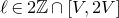 $\ell\in 2\mathbb{Z}\cap[V,2V]$
, by (3.12) we have
$\ell\in 2\mathbb{Z}\cap[V,2V]$
, by (3.12) we have
 \begin{align*} \nu(M_{\{\ell\}}(c_1,\ldots,c_m))\geqslant\mu(c_1,\ldots,c_m)\frac{T}{3K^2 V}\prod_{j=1}^\infty \bigg(1-\frac1{3j^{1+\delta}\psi(V)}\bigg)\geqslant\mu(c_1,\ldots,c_m)\frac{T}{4K^2 V} \end{align*}
for V large enough. Splitting into subintervals we then have that the same bound holds for any
 $m\leqslant \ell-1$
.
$m\leqslant \ell-1$
.
Next, we let
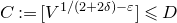 $C:= [V^{1/(2+2\delta)-\varepsilon}]\leqslant D$
and notice that if
$C:= [V^{1/(2+2\delta)-\varepsilon}]\leqslant D$
and notice that if
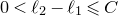 $0<\ell_2-\ell_1\leqslant C$
, then
$0<\ell_2-\ell_1\leqslant C$
, then
 $M_{\{\ell_1\}}(c_1,\ldots,c_m) \cap M_{\{\ell_2\}}(c_1,\ldots,c_m) = \emptyset$
. Indeed, if
$M_{\{\ell_1\}}(c_1,\ldots,c_m) \cap M_{\{\ell_2\}}(c_1,\ldots,c_m) = \emptyset$
. Indeed, if
 $x\in M_{\{\ell_1\}}(c_1,\ldots,c_m)$
, then
$x\in M_{\{\ell_1\}}(c_1,\ldots,c_m)$
, then
 $$b_{\ell_2}(x)\leqslant (\ell_2-\ell_1)^{1+\delta}\psi(V)\leqslant C^{1+\delta}V^\varepsilon<\sqrt{ V}$$
and thus
 $x\notin M_{\{\ell_2\}}(c_1,\ldots,c_m)$
. It follows that for any
$x\notin M_{\{\ell_2\}}(c_1,\ldots,c_m)$
. It follows that for any
 $W\in\mathbb{N}$
with
$W\in\mathbb{N}$
with
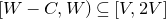 $[W-C,W)\subseteq [V,2V]$
, we have
$[W-C,W)\subseteq [V,2V]$
, we have
 \begin{align} \nu(M_{[W-C,W)}(c_1,\ldots,c_m))=\sum_{\ell\in I\cap 2\mathbb{Z}} \nu(M_{\{\ell\}}(c_1,\ldots,c_m))\geqslant \mu(c_1,\ldots,c_m)\frac{T {\lfloor {C/2} \rfloor}}{4K^2 V} \end{align}
for any
 $m<W-C$
.
$m<W-C$
.
Let
 $W\in\mathbb{N}$
with
$W\in\mathbb{N}$
with
 $V < W - 2D$
and
$V < W - 2D$
and
 $W\leqslant 2V$
, and let
$W\leqslant 2V$
, and let
 $m=W-C-1\geqslant W-D$
. We observe that the condition
$m=W-C-1\geqslant W-D$
. We observe that the condition
 $\ell\in G_V'(x)$
depends only on the first
$\ell\in G_V'(x)$
depends only on the first
 $\ell+D$
partial quotients of x. Thus, since
$\ell+D$
partial quotients of x. Thus, since
 $m\geqslant W-D$
, we have that
$m\geqslant W-D$
, we have that
 $M_{[V,W-2D)}(c_1,\ldots,c_m)$
is either empty or is equal to
$M_{[V,W-2D)}(c_1,\ldots,c_m)$
is either empty or is equal to
 $J(c_1,\ldots, c_m)$
. By (3.23), we deduce
$J(c_1,\ldots, c_m)$
. By (3.23), we deduce
 \begin{align*} \nu(M_{[V,W)})-\nu(M_{[V,W-2D)}) &{} = \nu(M_{[W-2D,W)}\smallsetminus M_{[V,W)}) \\ &{} \geqslant \nu(M_{[W-C,W)}\smallsetminus M_{[V,W-2D)})\\ &{} =\sum_{c_1,\ldots,c_m\geqslant 1\atop M_{[V,W-2D)}(c_1, \dotsc, c_m) = \emptyset}\nu(M_{[W-C,W)}(c_1,\ldots,c_m))\\ &{} \geqslant \frac{TC}{12K^2V}\sum_{c_1,\ldots,c_m\geqslant 1\atop M_{[V,W-2D)}(c_1, \dotsc, c_m) =\emptyset}\mu(c_1,\ldots,c_m) \\ &{} = \frac{TC}{12K^2 V}(1-\nu(M_{[V,W-2D)})). \end{align*}
We have used
 ${\lfloor {C/2} \rfloor}\geqslant C/3$
in the fourth line. We thus obtain
${\lfloor {C/2} \rfloor}\geqslant C/3$
in the fourth line. We thus obtain
 \begin{align*} 1-\nu(M_{[V,W)})\leqslant (1-\nu(M_{[V,W-2D)}))(1- {TC}/12V). \end{align*}
Iterating, we then obtain
 \begin{align*} 1-\nu(M_{[V,2V)})\leqslant (1- {TC}/12K^2V)^{[V/2D]}=o(1) \end{align*}
since
 $TC/K^2 D \asymp T V^{-1/(2+2\delta)-2\varepsilon}\to\infty$
if
$TC/K^2 D \asymp T V^{-1/(2+2\delta)-2\varepsilon}\to\infty$
if
 $\varepsilon$
is small enough.
$\varepsilon$
is small enough.
For
 $j\in\mathbb{N}$
and
$j\in\mathbb{N}$
and
 $K,\psi$
as in the lemma, we let
$K,\psi$
as in the lemma, we let
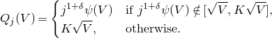 \begin{align*} Q_j(V)=\begin{cases} j^{1+\delta}\psi(V) & \text{if $j^{1+\delta}\psi(V)\notin[\sqrt V,K\sqrt V]$,}\\ K\sqrt V, &\text{otherwise.} \end{cases}\end{align*}
We then define
 $$G_V^*(x):=\{g\in [ V,2 V] \mid b_g(x)\in \mathscr{B}(e_{g-1}(x), v_{g-1}(x)),\, b_{g+j}(x)<Q_j(V)\ \forall j\geqslant1\}$$
and the corresponding set
 $X_{V,\mathscr{B}}$
. Clearly,
$X_{V,\mathscr{B}}$
. Clearly,
 $G_V^*(x)\supseteq G_V(x)$
and thus, under the hypothesis of Lemma 3.12,
$G_V^*(x)\supseteq G_V(x)$
and thus, under the hypothesis of Lemma 3.12,
 $\nu(X^*_{V,\mathscr{B}})=1+o(1)$
as
$\nu(X^*_{V,\mathscr{B}})=1+o(1)$
as
 $V\to\infty$
.
$V\to\infty$
.
We let
 $$ \kappa := \begin{cases} -{\beta} & \text{if } \operatorname{Im} k \neq 0, \\ 0 &\text{if }\operatorname{Im} k = 0, \end{cases} $$
and define the sets
 $\mathscr{B}$
as in (3.15). Also, we define
$\mathscr{B}$
as in (3.15). Also, we define
 $S^*_{g, (c_i)}=S^*_{g, (c_i), \mathscr{B}}$
as in (3.19), but with
$S^*_{g, (c_i)}=S^*_{g, (c_i), \mathscr{B}}$
as in (3.19), but with
 $G^*_V(x)$
in place of
$G^*_V(x)$
in place of
 $G_V(x)$
. The following lemma is an analogue of Lemma 3.10.
$G_V(x)$
. The following lemma is an analogue of Lemma 3.10.
Lemma 3.13. Assume that
 $g\in2\mathbb{Z}\cap[V,2V]$
with
$g\in2\mathbb{Z}\cap[V,2V]$
with
 $V\geqslant1$
sufficiently large. For all
$V\geqslant1$
sufficiently large. For all
 $c_1, \dotsc, c_{g-1},c \geqslant 1$
and
$c_1, \dotsc, c_{g-1},c \geqslant 1$
and
 $\varepsilon>0$
, we have
$\varepsilon>0$
, we have
 $$ \nu(\{ x\in S^*_{g, (c_i)} \colon {| {b_g(x) - c} |} \leqslant \varepsilon \sqrt{V} \}) \ll \varepsilon \xi^{-1} \nu(S^*_{g, (c_i)}), $$
where the constant depends on k,
 $\delta$
and N at most.
$\delta$
and N at most.
Proof. We may assume
 $S^*_{g, (c_i)} \neq \emptyset$
. Let
$S^*_{g, (c_i)} \neq \emptyset$
. Let
 $x'\in S^*_{g, (c_i)}$
. First we prove that for all
$x'\in S^*_{g, (c_i)}$
. First we prove that for all
 $c'\in\mathscr{B}(e_{g-1}(x'), v_{g-1}(x'))$
, we have
$c'\in\mathscr{B}(e_{g-1}(x'), v_{g-1}(x'))$
, we have
 \begin{equation} \{x\in S^*_{g, (c_i)} \colon b_g(x)=c'\} = \{x\in J(c_1,\ldots,c_{g-1},c') \mid b_{g+j}(x) < Q_j(V),\ j\geqslant1\}. \end{equation}
Any x in the left-hand side satisfies
 $g\in G_V^*(x)$
, and therefore
$g\in G_V^*(x)$
, and therefore
 $b_{g+j}(x) < Q_j(V)$
. The inclusion
$b_{g+j}(x) < Q_j(V)$
. The inclusion
 $\subseteq$
follows trivially. Consider then a number x in the right-hand side. The condition
$\subseteq$
follows trivially. Consider then a number x in the right-hand side. The condition
 $b_g(x)=c'$
is evident, and in order to prove the inclusion
$b_g(x)=c'$
is evident, and in order to prove the inclusion
 $\supseteq$
, there remains to show
$\supseteq$
, there remains to show
 $x\in S_{g, (c_i)}^*$
. Since
$x\in S_{g, (c_i)}^*$
. Since
 $x\in J(c_1, \dotsc, c_{g-1}, c')$
, it suffices to prove that
$x\in J(c_1, \dotsc, c_{g-1}, c')$
, it suffices to prove that
 $g\in G_V^*(x)$
and
$g\in G_V^*(x)$
and
 $\forall j\geqslant 1, g-2j \not\in G_V^*(x)$
. The condition
$\forall j\geqslant 1, g-2j \not\in G_V^*(x)$
. The condition
 $g\in G^*_V(x)$
holds since
$g\in G^*_V(x)$
holds since
 $c' \in \mathscr{B}(e_{g-1}(x'), v_{g-1}(x'))$
by hypothesis and
$c' \in \mathscr{B}(e_{g-1}(x'), v_{g-1}(x'))$
by hypothesis and
 $(e_{g-1}(x), v_{g-1}(x)) = (v_{g-1}(x'), e_{g-1}(x'))$
.
$(e_{g-1}(x), v_{g-1}(x)) = (v_{g-1}(x'), e_{g-1}(x'))$
.
Next, let
 $j\geqslant 1$
. We wish to show that
$j\geqslant 1$
. We wish to show that
 $g-2j\not\in G^*_V(x)$
. We assume that
$g-2j\not\in G^*_V(x)$
. We assume that
 $g-2j \in [V, 2V]$
; it suffices to prove that for such j, we have
$g-2j \in [V, 2V]$
; it suffices to prove that for such j, we have
 $b_{g-2j}(x)\not\in \mathscr{B}(e_{g-2j-1}(x), v_{g-2j-1}(x))$
or that
$b_{g-2j}(x)\not\in \mathscr{B}(e_{g-2j-1}(x), v_{g-2j-1}(x))$
or that
 $b_{g-2j+\ell}(x) \geqslant Q_\ell(V)$
for some
$b_{g-2j+\ell}(x) \geqslant Q_\ell(V)$
for some
 $\ell\geqslant1$
. We first prove that
$\ell\geqslant1$
. We first prove that
 \begin{equation} b_{g-2j}(x') \not\in \mathscr{B}(e_{g-2j-1}(x'), v_{g-2j-1}(x')) \quad \text{or} \quad \exists\ell\in\{1, \dotsc, 2j\}, b_{g-2j+\ell}(x') \geqslant Q_\ell(V). \end{equation}
Indeed, from the condition
 $g-2j\not\in G^*_V(x')$
, it suffices to prove that
$g-2j\not\in G^*_V(x')$
, it suffices to prove that
 $b_{g-2j+\ell}(x') < Q_\ell(V)$
, if
$b_{g-2j+\ell}(x') < Q_\ell(V)$
, if
 $\ell>2j$
, but this is immediate since the condition
$\ell>2j$
, but this is immediate since the condition
 $g\in G^*_V(x')$
implies
$g\in G^*_V(x')$
implies
 $b_{g-2j+\ell}(x') < Q_{\ell-2j}(V) \leqslant Q_\ell(V)$
. Now we argue that the conditions (3.25) hold with x’ replaced by x. Since x, x’ share the same first
$b_{g-2j+\ell}(x') < Q_{\ell-2j}(V) \leqslant Q_\ell(V)$
. Now we argue that the conditions (3.25) hold with x’ replaced by x. Since x, x’ share the same first
 $g-1$
CF coefficients, this is trivial except for the condition at
$g-1$
CF coefficients, this is trivial except for the condition at
 $\ell=2j$
, which involves
$\ell=2j$
, which involves
 $b_g$
. It suffices to check that
$b_g$
. It suffices to check that
 $b_g(x) \geqslant Q_{2j}(V) \iff b_g(x') \geqslant Q_{2j}(V)$
. By construction, we have
$b_g(x) \geqslant Q_{2j}(V) \iff b_g(x') \geqslant Q_{2j}(V)$
. By construction, we have
 $Q_{2j}(V) \not\in[\sqrt{V}, K\sqrt{V}]$
, so both conditions are in fact equivalent to
$Q_{2j}(V) \not\in[\sqrt{V}, K\sqrt{V}]$
, so both conditions are in fact equivalent to
 $Q_{2j}(V) \leqslant \sqrt{V}$
. This shows that the conditions (3.25) hold with x’ replaced by x, and therefore
$Q_{2j}(V) \leqslant \sqrt{V}$
. This shows that the conditions (3.25) hold with x’ replaced by x, and therefore
 $g-2j\not\in G^*_V(x)$
. This concludes the proof of the inclusion
$g-2j\not\in G^*_V(x)$
. This concludes the proof of the inclusion
 $\supseteq$
in (3.24).
$\supseteq$
in (3.24).
From there, the rest of the proof follows closely that of Lemma 3.10. By (3.12) and since
 $Q_j(V) \geqslant j^{1+\delta} \psi(V)$
, we deduce that
$Q_j(V) \geqslant j^{1+\delta} \psi(V)$
, we deduce that
 \begin{align*} \nu(\{x\in S^*_{g, (c_i)} \colon b_g(x)=c'\})&= \mu(c_1,\ldots,c_{g-1},c')\prod_{j\geqslant1}\bigg(1+O\bigg(\frac1 {j^{1+\delta}\psi(V)}\bigg)\bigg)\\ &= \mu(c_1,\ldots,c_{g-1},c')(1+o(1)) \end{align*}
as
 $V\to\infty$
. We conclude as for Lemma 3.10.
$V\to\infty$
. We conclude as for Lemma 3.10.
The following technical lemma allows us to extract values of h which will give a dominant contribution to
 $f^\triangleright$
.
$f^\triangleright$
.
Lemma 3.14. Let
 ${R}>1,C\geqslant1$
and
${R}>1,C\geqslant1$
and
 $\delta\in(0,1)$
. Let
$\delta\in(0,1)$
. Let
 $h:[-1,1]\smallsetminus\{0\}\to\mathbb{R}$
be such that
$h:[-1,1]\smallsetminus\{0\}\to\mathbb{R}$
be such that
 $h(x)\ll {e}^{|x|^{-1+\delta}}$
for
$h(x)\ll {e}^{|x|^{-1+\delta}}$
for
 $x\neq 0$
, and assume
$x\neq 0$
, and assume
 $|h(x)|\to\infty$
as
$|h(x)|\to\infty$
as
 $x\to 0^{\pm}$
for a choice of
$x\to 0^{\pm}$
for a choice of
 $\pm$
. Finally, let
$\pm$
. Finally, let
 $\xi:(0,1]\to (0,1]$
with
$\xi:(0,1]\to (0,1]$
with
 $\lim_{x\to0^+}\xi(x)=0$
. Then there exist
$\lim_{x\to0^+}\xi(x)=0$
. Then there exist
 $\nu>0$
and
$\nu>0$
and
 $\psi:[1,\infty)\to\mathbb{R}_{>0}$
with
$\psi:[1,\infty)\to\mathbb{R}_{>0}$
with
 $\lim_{+\infty}\psi = +\infty$
such that
$\lim_{+\infty}\psi = +\infty$
such that
 \begin{align} \sup_{(Cj^{-1-\delta} \psi(1/z))^{-1}<|x|<1}\frac{|h(x)|}{{R}^{j}}<\inf_{0<\pm y\leqslant \xi(z)}\frac{|h(y)|}{\psi (1/z)} \end{align}
for all
 $j\geqslant1$
and all
$j\geqslant1$
and all
 $z\in(0,\nu]$
.
$z\in(0,\nu]$
.
Proof. Assume
 $|h(x)|\to\infty$
as
$|h(x)|\to\infty$
as
 $x\to 0^+$
; the complementary case follows by changing h(x) to
$x\to 0^+$
; the complementary case follows by changing h(x) to
 $h(-x)$
. We fix a function
$h(-x)$
. We fix a function
 $\psi_1:(0,1]\to\mathbb{R}_{>0}$
going to
$\psi_1:(0,1]\to\mathbb{R}_{>0}$
going to
 $\infty$
at
$\infty$
at
 $0^+$
. By hypothesis, we have
$0^+$
. By hypothesis, we have
 $|h(x)|<\exp( C^{1-\delta} j^{1-\delta^2}\psi_1(z)^{1-\delta})$
for
$|h(x)|<\exp( C^{1-\delta} j^{1-\delta^2}\psi_1(z)^{1-\delta})$
for
 $z\in(0,\nu]$
,
$z\in(0,\nu]$
,
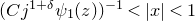 $(C{j^{1+\delta}\psi_1(z)})^{-1}<|x|<1$
and
$(C{j^{1+\delta}\psi_1(z)})^{-1}<|x|<1$
and
 $\nu>0$
sufficiently small. Now, for any
$\nu>0$
sufficiently small. Now, for any
 $z\in(0,1]$
the maximum
$z\in(0,1]$
the maximum
 $\psi_2(z):=\max_{j\in\mathbb{N}}({R}^{-j}\exp( C^{1-\delta} j^{1-\delta^2}\psi_1(z)^{1-\delta}))$
exists. Moreover, since
$\psi_2(z):=\max_{j\in\mathbb{N}}({R}^{-j}\exp( C^{1-\delta} j^{1-\delta^2}\psi_1(z)^{1-\delta}))$
exists. Moreover, since
 $\psi_1(z)$
goes to infinity as
$\psi_1(z)$
goes to infinity as
 $z\to 0^+$
, then clearly so does
$z\to 0^+$
, then clearly so does
 $\psi_2(z)$
. Also, by hypothesis we have
$\psi_2(z)$
. Also, by hypothesis we have
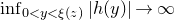 $\inf_{0<y<\xi(z)}|h(y)|\to\infty$
as
$\inf_{0<y<\xi(z)}|h(y)|\to\infty$
as
 $z\to0^+$
. It follows that we can ensure that
$z\to0^+$
. It follows that we can ensure that
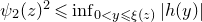 $\psi_2(z)^2\leqslant \inf_{0<y\leqslant \xi(z)}|h(y)|$
for
$\psi_2(z)^2\leqslant \inf_{0<y\leqslant \xi(z)}|h(y)|$
for
 $z\in (0, \nu]$
by taking
$z\in (0, \nu]$
by taking
 $\psi_1$
that goes to infinity sufficiently slowly and
$\psi_1$
that goes to infinity sufficiently slowly and
 $\nu$
small enough. By construction, for
$\nu$
small enough. By construction, for
 $z\in(0,\nu)$
and all
$z\in(0,\nu)$
and all
 $j\geqslant 1$
, we then have
$j\geqslant 1$
, we then have
 $$ \sup_{(C{j^{1+\delta}\psi_1(z)})^{-1}<|x|<1}\frac{|h(x)|}{{R}^j}<{R}^{-j}\exp( j^{1-\delta^2}\psi_1(z)^{1-\delta})\leqslant\psi_2(z)\leqslant \frac{\inf_{0<y\leqslant \xi(z)}{|h(y)|}}{\psi_2(z)}. $$
It is then sufficient to take
 $\psi(1/z):=\min(\psi_1(z),\psi_2(z)).$
We shall now show that if (2*) is satisfied then the CDF of
 $(\phi\circ f^\triangleright)_\ast( \nu)$
is continuous. We assume
$(\phi\circ f^\triangleright)_\ast( \nu)$
is continuous. We assume
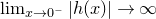 $\lim_{x\to 0^-}|h(x)|\to\infty$
, the other case being analogous.
$\lim_{x\to 0^-}|h(x)|\to\infty$
, the other case being analogous.
We take
 $R=\varpi^{\operatorname{Re}(k)/2}$
,
$R=\varpi^{\operatorname{Re}(k)/2}$
,
 $C=2K$
, where K was defined at (3.15), and
$C=2K$
, where K was defined at (3.15), and
 $\xi(w):=w^{-1/2}$
, and we apply Lemma 3.14, thus finding a constant
$\xi(w):=w^{-1/2}$
, and we apply Lemma 3.14, thus finding a constant
 $\nu>0$
and a function
$\nu>0$
and a function
 $\psi(x)$
with the properties claimed in this lemma. We then apply Lemma 3.12 with the same function
$\psi(x)$
with the properties claimed in this lemma. We then apply Lemma 3.12 with the same function
 $\psi$
. As in the bounded case, for any
$\psi$
. As in the bounded case, for any
 $g\in [V, 2V]\cap 2\mathbb{Z}$
and
$g\in [V, 2V]\cap 2\mathbb{Z}$
and
 $c_1, \dotsc, c_{g-1}\geqslant 1$
, the sets
$c_1, \dotsc, c_{g-1}\geqslant 1$
, the sets
 $(S^*_{g, (c_i)})$
are disjoint and, given any fixed
$(S^*_{g, (c_i)})$
are disjoint and, given any fixed
 $\varepsilon>0$
, their union has measure
$\varepsilon>0$
, their union has measure
 $\geqslant1-\varepsilon$
, if V is large enough in terms of
$\geqslant1-\varepsilon$
, if V is large enough in terms of
 $\varepsilon$
.
$\varepsilon$
.
For any
 $x\in S^*_{g, (c_i)}$
and any
$x\in S^*_{g, (c_i)}$
and any
 $j\geqslant1$
, we have
$j\geqslant1$
, we have
 $$\frac{v_{g+j-1}}{v_{g+j}}\geqslant \frac 1{2b_{g+j}}\geqslant \frac{1}{2Q_j(V)}\geqslant \frac{1}{2K\psi(V) j^{1+\delta}},$$
where we dropped the dependency on x in the inequalities for ease of notation. Thus, assuming
 $V>1/\nu$
, by (3.26) (with
$V>1/\nu$
, by (3.26) (with
 $z=1/V$
) we have
$z=1/V$
) we have
 $$\frac{|h((-1)^{j-1}{v_{g+j-1}}/{v_{g+j}})|}{\varpi^{\operatorname{Re}(k)j}}< \inf_{0< z\leqslant 1/\sqrt V}\frac{|h(-z)|}{\varpi^{\operatorname{Re}(k)j/2}\psi(V)}\leqslant \frac{|h(-{v_{g-1}}/{v_g})|}{\varpi^{\operatorname{Re}(k)j/2}\psi(V)},$$
since
 $v_{g-1}/v_g\leqslant 1/b_g\leqslant 1/\sqrt V$
. With
$v_{g-1}/v_g\leqslant 1/b_g\leqslant 1/\sqrt V$
. With
 $F_g(x)$
as in (3.20) we then deduce the following analogue of (3.21),
$F_g(x)$
as in (3.20) we then deduce the following analogue of (3.21),
 \begin{align*} F_g(x) &= \frac{\vartheta^p h(-{v_{g-1}(x)}/{v_g(x)})}{v_g(x)^{k}}+O\bigg(\sum_{j\geqslant1}^\infty \frac{|h((-1)^{j-1}{v_{g+j-1}(x)}/{v_{g+j}(x)})}{ v_g(x)^{\operatorname{Re}(k)}\varpi^{\operatorname{Re}(k)j}}\bigg)\\ &=\frac{\vartheta^p+o(1)}{v_g(x)^{k}}h(-{v_{g-1}(x)}/{v_g(x)}).\end{align*}
We let
 $x,y\in S^*_{g, (c_i)}$
and write
$x,y\in S^*_{g, (c_i)}$
and write
 $${u}_g=\frac{v_{g}(x)}{v_{g}(y)}=\frac{b_{g}(x)v_{g-1}+v_{g-2}}{b_{g}(y)v_{g-1}+v_{g-2}}$$
and
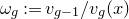 $\omega_g:=v_{g-1}/v_{g}(x)$
, so that we have
$\omega_g:=v_{g-1}/v_{g}(x)$
, so that we have
 \begin{align*} F_g(x)-F_g(y) &=\vartheta^p\frac{ |h(-\omega_g)|}{v_g(x)^k}\bigg( \frac{h(-\omega_g)-{u}_g^kh(-{u}_g \omega_g)}{ |h(-\omega_g)|}+o(1)\bigg).\end{align*}
By the definition of
 $\mathscr{B}$
we have
$\mathscr{B}$
we have
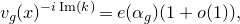 $$v_g(x)^{-i\operatorname{Im}(k)}={e}(\alpha_g)(1+o(1)),$$
with
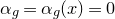 $\alpha_g=\alpha_g(x)=0$
if
$\alpha_g=\alpha_g(x)=0$
if
 $\operatorname{Im}(k)=0$
and otherwise
$\operatorname{Im}(k)=0$
and otherwise
 $\alpha_g(x)$
satisfying
$\alpha_g(x)$
satisfying
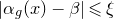 $|\alpha_g(x) - {\beta}| \leqslant \xi$
. Moreover,
$|\alpha_g(x) - {\beta}| \leqslant \xi$
. Moreover,
 $\log {u}_g = \log (b_g(x)/b_g(y)) + o(1) \ll_k \xi$
and, if
$\log {u}_g = \log (b_g(x)/b_g(y)) + o(1) \ll_k \xi$
and, if
 $|b_g(x)-b_{g}(y)|> \varepsilon \sqrt V$
, then also
$|b_g(x)-b_{g}(y)|> \varepsilon \sqrt V$
, then also
 $|\log {u}_g|\geqslant \log(1+\varepsilon/K) + o(1) \gg_k \varepsilon$
for V large enough. Taking
$|\log {u}_g|\geqslant \log(1+\varepsilon/K) + o(1) \gg_k \varepsilon$
for V large enough. Taking
 $\xi=\varepsilon^{2/3}$
we then have
$\xi=\varepsilon^{2/3}$
we then have
 \begin{align} \phi( F_g(x)-F_g(y)) &=\frac{ |h(-\omega_g)|}{|v_g(x)|^k} \phi\bigg(\vartheta^p{e}(\alpha_g)\bigg( \frac{h(-\omega_g)-{u}_g^kh(-{u}_g \omega_g)}{ |h(-\omega_g)|}\bigg)+o(1)\bigg)\\ &\neq0\notag\end{align}
by hypothesis (2*), provided that
 $|b_g(x)-b_{g}(y)|> \varepsilon \sqrt V$
. We then conclude in the same way as we did in § 3.3.1.
$|b_g(x)-b_{g}(y)|> \varepsilon \sqrt V$
. We then conclude in the same way as we did in § 3.3.1.
Remark 3.15. From the above proof, it is clear that the term o(1) in (3.27) can be replaced by
 $O(1/\sqrt{V} + 1/\psi(V))$
. This will be used in one special case of our applications to the cotangent sums.
$O(1/\sqrt{V} + 1/\psi(V))$
. This will be used in one special case of our applications to the cotangent sums.
Remark 3.16. From the above proof, it is also immediate to see that we can modify the condition
 $(2^*)$
,
$(2^*)$
,
 $k\not \in\mathbb{R}$
, of Theorem 3.5 as follows. Given
$k\not \in\mathbb{R}$
, of Theorem 3.5 as follows. Given
 $\beta\in\mathbb{R}$
and any small
$\beta\in\mathbb{R}$
and any small
 $\varepsilon>0$
, we denote by
$\varepsilon>0$
, we denote by
 $\mathcal R=\mathcal R_{k,\varepsilon,\beta}$
the set or reduced rationals
$\mathcal R=\mathcal R_{k,\varepsilon,\beta}$
the set or reduced rationals
 $x=p/q$
with
$x=p/q$
with
 $|q^{-i\operatorname{Im}(k)}{e}(-\beta)-1|\leqslant 10\varepsilon^{2/3}.$
Then, we can weaken the condition
$|q^{-i\operatorname{Im}(k)}{e}(-\beta)-1|\leqslant 10\varepsilon^{2/3}.$
Then, we can weaken the condition
 $\lim_{x\to0^\pm}|h(x)|=\infty$
in
$\lim_{x\to0^\pm}|h(x)|=\infty$
in
 $(2^*)$
by introducing the restriction
$(2^*)$
by introducing the restriction
 $x\in \mathcal R$
in the limit and replace (3.7) by
$x\in \mathcal R$
in the limit and replace (3.7) by
 \begin{equation*} \liminf_{x\to 0^\pm\atop x\in \mathcal R} \inf\bigg\{\bigg|\phi\bigg({e}(\alpha) \frac{ h(x)- {u}^{k} h({u} x)}{|h(x)|} \bigg)\bigg|: {\begin{aligned} & |\log u| \in (\varepsilon, \varepsilon^{2/3}), |\alpha-{\beta}| \lt \varepsilon^{2/3}\\ & {u} x \in \mathcal{R}, \textrm{Num}({u} x)=\textrm{Num}(x)\\ \end{aligned}}\bigg\} > 0. \end{equation*}
4. Arithmetic applicationsFootnote 6
4.1 Eichler integrals of holomorphic cusp forms
Proof of Corollary 1.10. The map
 $f(x) = \widetilde g(x)$
satisfies the relation (1.2) with weight
$f(x) = \widetilde g(x)$
satisfies the relation (1.2) with weight
 $2-k$
and with h being a non-zero polynomial of degree at most
$2-k$
and with h being a non-zero polynomial of degree at most
 $k-2$
, see [Reference EichlerEic57, p. 273]. Since h is Lipschitz and bounded on
$k-2$
, see [Reference EichlerEic57, p. 273]. Since h is Lipschitz and bounded on
 $[-1, 1]$
, the estimates (1.5) hold trivially. We may therefore apply Theorem 1.3, which gives the claimed convergence in distribution. Notice that in this case
$[-1, 1]$
, the estimates (1.5) hold trivially. We may therefore apply Theorem 1.3, which gives the claimed convergence in distribution. Notice that in this case
 $\widetilde g^\triangleleft$
coincides on the whole real line with
$\widetilde g^\triangleleft$
coincides on the whole real line with
 $\widetilde g$
as defined in (1.10).
$\widetilde g$
as defined in (1.10).
Finally, assume
 $(\phi\circ \widetilde g^\triangleleft)_\ast( \nu)$
has an atom for some non-zero linear form
$(\phi\circ \widetilde g^\triangleleft)_\ast( \nu)$
has an atom for some non-zero linear form
 $\phi$
and write
$\phi$
and write
 $\phi(z)=\operatorname{Re}({e}^{i\theta}z)$
for some
$\phi(z)=\operatorname{Re}({e}^{i\theta}z)$
for some
 $\theta\in\mathbb{R}$
and all
$\theta\in\mathbb{R}$
and all
 $z\in\mathbb{C}$
. Then, by Proposition 3.4, we obtain that
$z\in\mathbb{C}$
. Then, by Proposition 3.4, we obtain that
 $\phi\circ \widetilde g^\triangleleft$
is constant on [0,1]. By (1.10),
$\phi\circ \widetilde g^\triangleleft$
is constant on [0,1]. By (1.10),
 $\phi\circ \widetilde g^\triangleleft$
is given by the Fourier series
$\phi\circ \widetilde g^\triangleleft$
is given by the Fourier series
 \begin{align*} x\mapsto \sum_{n\geqslant1}\frac{\operatorname{Re}(e^{i\theta} a_n)}{n^{k-1}}\cos(nx)-\sum_{n\geqslant1}\frac{\operatorname{Im}(e^{i\theta} a_n)}{n^{k-1}}\sin(nx), \end{align*}
which is constant on [0,1] only if
 $\operatorname{Re}(e^{i\theta} a_n)=\operatorname{Im}(e^{i\theta} a_n)=0$
, i.e.
$\operatorname{Re}(e^{i\theta} a_n)=\operatorname{Im}(e^{i\theta} a_n)=0$
, i.e.
 $a_n=0$
, for all
$a_n=0$
, for all
 $n\in\mathbb{N}_{>0}$
. Thus
$n\in\mathbb{N}_{>0}$
. Thus
 $g=0$
which was excluded by hypothesis.
$g=0$
which was excluded by hypothesis.
Proof of Corollary 1.9. The map
 $A_{k,D}$
defined in (1.9) coincides with
$A_{k,D}$
defined in (1.9) coincides with
 $F_{k+1, D}$
defined in [Reference ZagierZag99, Equation (15)]. Consider the even cusp form
$F_{k+1, D}$
defined in [Reference ZagierZag99, Equation (15)]. Consider the even cusp form
 $g = f_{k+1, D} \in S_{2k+2}(1)$
defined in [Reference ZagierZag99, Equation (53)]. By [Reference ZagierZag99, Equation (55)], we have
$g = f_{k+1, D} \in S_{2k+2}(1)$
defined in [Reference ZagierZag99, Equation (53)]. By [Reference ZagierZag99, Equation (55)], we have
 $A_{k,D}(x) = c_{k,D} + \frac12 \widetilde g(x)$
for all
$A_{k,D}(x) = c_{k,D} + \frac12 \widetilde g(x)$
for all
 $x\in\mathbb{Q}$
and some
$x\in\mathbb{Q}$
and some
 $c_{k, D} \in \mathbb{R}$
. Therefore, Corollary 1.9 follows from the just proved Corollary 1.10.
$c_{k, D} \in \mathbb{R}$
. Therefore, Corollary 1.9 follows from the just proved Corollary 1.10.
4.2 Kontsevich’s functionFootnote 7
Proof of Corollary 1.12. Define h by formula (1.13). In [Reference ZagierZag01, Theorem, p. 958], it is proved that
 $h\in C^\infty(\mathbb{R})$
and that h is real-analytic except at 0, and moreover
$h\in C^\infty(\mathbb{R})$
and that h is real-analytic except at 0, and moreover
 $h(0) = 1$
. Thus,
$h(0) = 1$
. Thus,
 $\varphi$
and h satisfy the hypotheses of the first part of Theorem 1.7, with the generalized hypotheses (2.26) (with
$\varphi$
and h satisfy the hypotheses of the first part of Theorem 1.7, with the generalized hypotheses (2.26) (with
 $\vartheta = {e}(1/24)$
) which were adopted in the proof. This proves the existence of the limiting distribution. The limit (1.14) arises from the relations (2.29) and (2.32).
$\vartheta = {e}(1/24)$
) which were adopted in the proof. This proves the existence of the limiting distribution. The limit (1.14) arises from the relations (2.29) and (2.32).
Let
 $\theta \in \mathbb{R}$
and
$\theta \in \mathbb{R}$
and
 $\phi: z \mapsto \operatorname{Re}({e}^{i\theta} z)$
. To see that
$\phi: z \mapsto \operatorname{Re}({e}^{i\theta} z)$
. To see that
 $(\phi \circ \varphi^\triangleright)_\ast(\nu)$
does not have atoms, we apply Theorem 3.5. The period function h is continuous on
$(\phi \circ \varphi^\triangleright)_\ast(\nu)$
does not have atoms, we apply Theorem 3.5. The period function h is continuous on
 $[-1, 1]$
, and
$[-1, 1]$
, and
 $h(0)=1$
. Since
$h(0)=1$
. Since
 $\vartheta\not\in\mathbb{R}$
, certainly one of
$\vartheta\not\in\mathbb{R}$
, certainly one of
 $\phi(1)$
or
$\phi(1)$
or
 $\phi(\vartheta)$
is non-zero, and therefore hypothesis (1*) is satisfied for some
$\phi(\vartheta)$
is non-zero, and therefore hypothesis (1*) is satisfied for some
 $p\in\{0, 1\}$
. Theorem 3.5 applies and yields the desired conclusion.
$p\in\{0, 1\}$
. Theorem 3.5 applies and yields the desired conclusion.
Finally, the continuity of
 $\varphi^\triangleright$
follows immediately from (the twisted version of) Theorem 1.4.
$\varphi^\triangleright$
follows immediately from (the twisted version of) Theorem 1.4.
4.3 Cotangent sums
For
 $b\in\mathbb{Z}$
,
$b\in\mathbb{Z}$
,
 $q\geqslant 1$
and
$q\geqslant 1$
and
 $(b, q) = 1$
, the cotangent sums we are interested in are defined by
$(b, q) = 1$
, the cotangent sums we are interested in are defined by
 $$ c_a\bigg(\frac bq\bigg) := q^a \sum_{m=1}^{q-1} \cot\bigg(\frac{\pi m b}{q}\bigg) \zeta\bigg(-a, \frac mq\bigg), $$
see [Reference Bettin and ConreyBC13a, p. 226]. The special case
 $a=-1$
corresponds to the classical Dedekind sums [Reference RiemannRie92, p. 466], while the case
$a=-1$
corresponds to the classical Dedekind sums [Reference RiemannRie92, p. 466], while the case
 $a=0$
corresponds to the cotangent sum from [Reference Bettin and ConreyBC13b]. These sums were described as ‘imperfect’ quantum modular forms, due to an irregular term arising in the period relation, namely the last term on the right-hand side of [Reference Bettin and ConreyBC13a, Equation (17)]; see the discussion in Example 0 in [Reference ZagierZag10]. The point of the upcoming definition is that we can relax this lack of regularity at the cost of weakening the periodicity hypothesis to (1.4). Let
$a=0$
corresponds to the cotangent sum from [Reference Bettin and ConreyBC13b]. These sums were described as ‘imperfect’ quantum modular forms, due to an irregular term arising in the period relation, namely the last term on the right-hand side of [Reference Bettin and ConreyBC13a, Equation (17)]; see the discussion in Example 0 in [Reference ZagierZag10]. The point of the upcoming definition is that we can relax this lack of regularity at the cost of weakening the periodicity hypothesis to (1.4). Let
 $$ \rho\bigg(\frac bq\bigg) = \begin{cases} \bigg\{\dfrac{\overline b}q\bigg\} & (q>1, (b, q)=1), \\ 1 & (q = 1, b>0), \\ 0 & (q=1, b<0). \end{cases} $$
By Bezout’s theorem, we have for
 $b\neq 0$
,
$b\neq 0$
,
 $q\geqslant 1$
,
$q\geqslant 1$
,
 $(b, q)=1$
,
$(b, q)=1$
,
 $$ \rho\bigg(\frac bq\bigg) - \rho\bigg(\frac{-q}{b}\bigg) = \frac1{bq}. $$
For
 $x\in\mathbb{Q}$
, let
$x\in\mathbb{Q}$
, let
 $$ {\widetilde c}_a(x) := c_a(x) + a\kappa_1(a) \operatorname{Den}(x)^{1+a} \rho(x) \quad (x\neq0),$$
extended arbitrarily at 0, and with
 $\kappa_1(a):=({\zeta(1-a)})/{\pi}$
. Note that
$\kappa_1(a):=({\zeta(1-a)})/{\pi}$
. Note that
 $c_a$
is 1-periodic, and that
$c_a$
is 1-periodic, and that
 $\rho$
satisfies the weak periodicity (1.4), from which we deduce that
$\rho$
satisfies the weak periodicity (1.4), from which we deduce that
 ${\widetilde c}_a$
also satisfies (1.4).
${\widetilde c}_a$
also satisfies (1.4).
From [Reference Bettin and ConreyBC13a, Theorem 4], we have
 \begin{equation} c_a(x) - {| {x} |}^{-1-a} c_a(-1/x) =h_a(x)-a\kappa_1(a)\frac{\operatorname{Den}(x)^a}{\textrm{Num}(x)} \quad (x \in \mathbb{Q}\smallsetminus\{0\}),\end{equation}
and thus
 \begin{equation} {\widetilde c}_a(x) - {| {x} |}^{-1-a} {\widetilde c}_a(-1/x) =h_a(x) \quad (x \in \mathbb{Q}\smallsetminus\{0\}),\end{equation}
for
 $h_a(x) := - \textrm{sgn}(x) i \zeta(-a) \psi_a({| {x} |})$
with
$h_a(x) := - \textrm{sgn}(x) i \zeta(-a) \psi_a({| {x} |})$
with
 $\psi_a(x)$
as in [Reference Bettin and ConreyBC13a, Theorem 4]. In particular,
$\psi_a(x)$
as in [Reference Bettin and ConreyBC13a, Theorem 4]. In particular,
 $h_a$
is real analytic on
$h_a$
is real analytic on
 $\mathbb{R}_{\neq0}$
. Also, by the same theorem, for
$\mathbb{R}_{\neq0}$
. Also, by the same theorem, for
 $a\neq0$
, we haveFootnote
8
$a\neq0$
, we haveFootnote
8
 \begin{equation} h_a(x) = \kappa_2(a)\textrm{sgn}(x) |x|^{-1-a} + \kappa_1(a) x^{-1}+O_a(|x|)\end{equation}
as
 $x\to 0$
, for
$x\to 0$
, for
 $\kappa_2(a)=-\zeta(-a)\cot({\pi a}/2)$
, and where the error has to be replaced by
$\kappa_2(a)=-\zeta(-a)\cot({\pi a}/2)$
, and where the error has to be replaced by
 $O({| {x} |}\log {| {1/x} |})$
if
$O({| {x} |}\log {| {1/x} |})$
if
 $a=-2$
. For
$a=-2$
. For
 $a=0$
, we instead have
$a=0$
, we instead have
 \begin{equation} h_0(x) = -\frac{\log(2\pi |x|)-\gamma}{\pi x}+ O(|x|).\end{equation}
We prove the distributional statements in Corollary 1.14, considering several cases depending on the value of a. The statement in Corollary 1.14 about the continuity of
 $c_a^\triangleright$
when
$c_a^\triangleright$
when
 $\operatorname{Re}(a)>0$
will follow immediately from Theorem 1.4 and the behavior around 0 of the period functions.
$\operatorname{Re}(a)>0$
will follow immediately from Theorem 1.4 and the behavior around 0 of the period functions.
4.3.1 The case
$\operatorname{Re}(a)<-1$
.

By [Reference Bettin and ConreyBC13a, Theorem 1], it follows that both
 $h_a$
and
$h_a$
and
 $h_a'$
are bounded by
$h_a'$
are bounded by
 ${| {x} |}^{O(1)}$
for all
${| {x} |}^{O(1)}$
for all
 $x\neq 0$
. Thus, the conditions (1.5) are satisfied, and by Theorem 1.2, the function
$x\neq 0$
. Thus, the conditions (1.5) are satisfied, and by Theorem 1.2, the function
 \begin{equation} {\widetilde c}_a^\triangleleft(x) = \lim_{j\to \infty} {\widetilde c}_a([b_0; b_1, \dotsc, b_j]) \quad (x=[b_0;b_1, b_2, \dotsc])\end{equation}
exists for x in a full measure set
 $X\subset \mathbb{R}$
. By Theorem 1.3, we deduce that the multisets
$X\subset \mathbb{R}$
. By Theorem 1.3, we deduce that the multisets
 $$ \{{\widetilde c}_a(b/q),\ 0<b<q, (b, q) = 1\} $$
become equidistributed, as
 $q\to\infty$
, according to
$q\to\infty$
, according to
 $({\widetilde c}_a^\triangleleft)_*( \nu)$
. Since
$({\widetilde c}_a^\triangleleft)_*( \nu)$
. Since
 \begin{equation} {\widetilde c}_a(x) - c_a(x) = O(\operatorname{Den}(x)^{1+\operatorname{Re}(a)}) = o_a(1)\end{equation}
as
 $\operatorname{Den}(x) \to \infty$
, uniformly in the numerator
$\operatorname{Den}(x) \to \infty$
, uniformly in the numerator
 $\textrm{Num}(x)$
, it follows that the same conclusion holds for the multisets
$\textrm{Num}(x)$
, it follows that the same conclusion holds for the multisets
 $$ \bigg\{c_a\bigg(\frac bq\bigg),\ 0<b<q, (b, q) = 1\bigg\}. $$
Next we prove that if
 $a\in\mathbb{R}_{<-1}$
, then
$a\in\mathbb{R}_{<-1}$
, then
 $({\widetilde c}_a^\triangleleft)_*(\nu)$
is diffuse on
$({\widetilde c}_a^\triangleleft)_*(\nu)$
is diffuse on
 $\mathbb{R}$
. Assume, for the sake of contradiction, the existence of
$\mathbb{R}$
. Assume, for the sake of contradiction, the existence of
 $\lambda\in\mathbb{R}$
and
$\lambda\in\mathbb{R}$
and
 $C\subset X\cap\mathbb{R}_{>0}$
of positive Lebesgue measure such that
$C\subset X\cap\mathbb{R}_{>0}$
of positive Lebesgue measure such that
 ${\widetilde c}_a^\triangleleft(x) = \lambda$
for all
${\widetilde c}_a^\triangleleft(x) = \lambda$
for all
 $x\in C$
. By Proposition 3.4, we deduce that
$x\in C$
. By Proposition 3.4, we deduce that
 ${\widetilde c}_a^\triangleleft(x) = \lambda$
for almost all
${\widetilde c}_a^\triangleleft(x) = \lambda$
for almost all
 $x>0$
. Using the fact that
$x>0$
. Using the fact that
 $c_a$
is odd, which transfers to
$c_a$
is odd, which transfers to
 ${\widetilde c}_a^\triangleleft$
almost everywhere by (4.6), we obtain by the period relation (4.2) that
${\widetilde c}_a^\triangleleft$
almost everywhere by (4.6), we obtain by the period relation (4.2) that
 $h_a(x)=\lambda (1+ {| {x} |}^{-1-a} )$
for almost all
$h_a(x)=\lambda (1+ {| {x} |}^{-1-a} )$
for almost all
 $x>0$
. However, this contradicts (4.3) as
$x>0$
. However, this contradicts (4.3) as
 $x\to 0^+$
, regardless of the value of a.
$x\to 0^+$
, regardless of the value of a.
Now, let
 $a\notin\mathbb{R}$
and let
$a\notin\mathbb{R}$
and let
 $\phi:\mathbb{C}\to\mathbb{R}$
a non-zero linear form. We assume by contradiction that
$\phi:\mathbb{C}\to\mathbb{R}$
a non-zero linear form. We assume by contradiction that
 $(\phi\circ{\widetilde c}_a^\triangleleft)_*(\nu)$
is not diffuse. As above, we deduce that there exists
$(\phi\circ{\widetilde c}_a^\triangleleft)_*(\nu)$
is not diffuse. As above, we deduce that there exists
 $\lambda\in\mathbb{R}$
such that
$\lambda\in\mathbb{R}$
such that
 $\phi({\widetilde c}_a^\triangleleft(x)) = \lambda$
for almost all
$\phi({\widetilde c}_a^\triangleleft(x)) = \lambda$
for almost all
 $x>0$
. Composing the period relation (4.2) with
$x>0$
. Composing the period relation (4.2) with
 $\phi$
, we obtain
$\phi$
, we obtain
 $\phi(h_a(x))= \lambda - \phi( {| {x} |}^{-1-a} {\widetilde c}_a^\triangleleft(-1/x))$
. We pick
$\phi(h_a(x))= \lambda - \phi( {| {x} |}^{-1-a} {\widetilde c}_a^\triangleleft(-1/x))$
. We pick
 $y\in(0, 1)$
so that
$y\in(0, 1)$
so that
 ${\widetilde c}_a^\triangleleft(-y)$
and
${\widetilde c}_a^\triangleleft(-y)$
and
 ${\widetilde c}_a^\triangleleft(1/(n+y))$
are defined in (4.5) for all
${\widetilde c}_a^\triangleleft(1/(n+y))$
are defined in (4.5) for all
 $n\in\mathbb{N}_{>0}$
, and
$n\in\mathbb{N}_{>0}$
, and
 $\phi({\widetilde c}_a^\triangleleft(1/(n+y))) = \lambda$
. Taking
$\phi({\widetilde c}_a^\triangleleft(1/(n+y))) = \lambda$
. Taking
 $x=1/(n+y)$
, by periodicity we then obtain
$x=1/(n+y)$
, by periodicity we then obtain
 \begin{align} \phi(h_a(x))=\lambda - \phi( {| {n+y} |}^{1+a} {\widetilde c}_a^\triangleleft(-y)).\end{align}
Now, by [Reference Bettin and ConreyBC13a, Theorem 1],Footnote 9 the asymptotic in (4.3) can be extended to
 \begin{equation} h_a(x) = \frac{\kappa_2(a)\textrm{sgn}(x)}{ |x|^{1+a}} + \frac{\kappa_1(a)}{ x}+\sum_{m=1}^M(-1)^m\frac{2B_{2m}}{(2m)!}\zeta(1-2m-a)(2\pi x)^{2m-1}+O_{a,M}(|x|^{2M+1}),\end{equation}
for any
 $M\in\mathbb{N}$
, where
$M\in\mathbb{N}$
, where
 $B_{2n}\in\mathbb{Q}_{\neq0}$
denotes the 2nth Bernoulli number. By the functional equation we have
$B_{2n}\in\mathbb{Q}_{\neq0}$
denotes the 2nth Bernoulli number. By the functional equation we have
 $$\frac{\zeta(1-2m-a)}{\zeta(1-2(m+1)-a)} =-\frac{2\pi}{(2m+a)(2m+a+1)}\frac{ \zeta(2m+a)}{ \zeta(2m+2+a)}=\frac{2\pi}{4m^2}\bigg(2-\frac{1+2a}{m}+O(m^{-2})\bigg)$$
as
 $m\to\infty$
. In particular,
$m\to\infty$
. In particular,
 $\zeta(1-2m-a)$
cannot be a real multiple of
$\zeta(1-2m-a)$
cannot be a real multiple of
 $\zeta(1-2(m+1)-a)$
for m large enough and thus at least one of these terms in the expansion (4.8) survives once composed with
$\zeta(1-2(m+1)-a)$
for m large enough and thus at least one of these terms in the expansion (4.8) survives once composed with
 $\phi$
. Letting
$\phi$
. Letting
 $n\to\infty$
, we see that this is not compatible with (4.7) and thus we reach a contradiction. This finishes the proof of Corollary 1.14 when
$n\to\infty$
, we see that this is not compatible with (4.7) and thus we reach a contradiction. This finishes the proof of Corollary 1.14 when
 $\operatorname{Re}(a)<-1$
.
$\operatorname{Re}(a)<-1$
.
4.3.2 The case
$\operatorname{Re}(a)>-1$
and
$a\zeta(a)\neq0$
.


It is remarked in [Reference Bettin and ConreyBC13a, p. 227] that
 $c_a(x) \equiv 0$
whenever a is a positive odd integer. In this case, Corollary 1.14 holds for trivial reasons and thus we assume that
$c_a(x) \equiv 0$
whenever a is a positive odd integer. In this case, Corollary 1.14 holds for trivial reasons and thus we assume that
 $a\not\in 2\mathbb{Z} + 1$
throughout the section. We also assume
$a\not\in 2\mathbb{Z} + 1$
throughout the section. We also assume
 $\operatorname{Re}(a)>-1$
and
$\operatorname{Re}(a)>-1$
and
 $a\zeta(a)\neq0$
and notice that by the functional equation we have
$a\zeta(a)\neq0$
and notice that by the functional equation we have
 $\kappa_1(a)\neq0$
.
$\kappa_1(a)\neq0$
.
Since
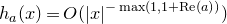 $ h_a(x) = O({| {x} |}^{-\max(1, 1+\operatorname{Re}(a))})$
for
$ h_a(x) = O({| {x} |}^{-\max(1, 1+\operatorname{Re}(a))})$
for
 ${| {x} |}<1$
, the hypotheses of Theorem 1.7 are satisfied and it follows that the limit
${| {x} |}<1$
, the hypotheses of Theorem 1.7 are satisfied and it follows that the limit
 \begin{align} {\widetilde c}_a^\triangleright(x) := \lim_{j\to\infty} \operatorname{Den}(x_{2j+1})^{-1-a} {\widetilde c}_a(\overline{x_{2j+1}}) \quad (x_{2j+1}=[b_0(x); b_1(x), \dotsc, b_{2j+1}(x)])\end{align}
exists for x in a full measure set
 $X\subset \mathbb{R}\smallsetminus\mathbb{Q}$
. By Theorem 1.7, we have that the multiset
$X\subset \mathbb{R}\smallsetminus\mathbb{Q}$
. By Theorem 1.7, we have that the multiset
 $$ \{q^{-1-a} {\widetilde c}_a( b/q) \colon 0<b<q, (b, q) = 1\}= \{q^{-1-a} {\widetilde c}_a( {\overline b}/q) \colon 0<b<q, (b, q) = 1\} $$
becomes distributed, as
 $q\to\infty$
, according to
$q\to\infty$
, according to
 $({\widetilde c}_a^\triangleright)_*( \nu)$
. But by definition of
$({\widetilde c}_a^\triangleright)_*( \nu)$
. But by definition of
 ${\widetilde c}_a$
, we have
${\widetilde c}_a$
, we have
 $q^{-1-a} {\widetilde c}_a({\overline b}/q)=q^{-1-a} c_a({\overline b}/q)+a\kappa_1(a)\{b/q\}$
for
$q^{-1-a} {\widetilde c}_a({\overline b}/q)=q^{-1-a} c_a({\overline b}/q)+a\kappa_1(a)\{b/q\}$
for
 $q>1$
. Letting
$q>1$
. Letting
 \begin{align} c_a^\triangleright(x) := {\widetilde c}_a^\triangleright(x) - a\kappa_1(a) \{x\},\end{align}
it follows that the multiset
 $$ \{q^{-1-a} c_a(b/q) \colon 0<b<q, (b, q) = 1\} $$
becomes distributed according to
 $(c_a^\triangleright)_*( \nu)$
, as claimed.
$(c_a^\triangleright)_*( \nu)$
, as claimed.
We now turn to showing that the relevant measures are diffuse.
It is convenient to make a further simple modification to
 $c_a$
and define
$c_a$
and define
 $ {\breve c}_a(x) := {\widetilde c}_a(x)-\kappa_2(a)\textrm{sgn}(x)$
. Clearly, one has that
$ {\breve c}_a(x) := {\widetilde c}_a(x)-\kappa_2(a)\textrm{sgn}(x)$
. Clearly, one has that
 ${\breve c}_a(x)$
still satisfies (1.4), whereas (4.2) holds with
${\breve c}_a(x)$
still satisfies (1.4), whereas (4.2) holds with
 $h_a(x)$
replaced by
$h_a(x)$
replaced by
 $\breve h_a(x)=h_a(x)-\kappa_1(a)(1+ {| {x} |}^{-1-a})$
. In particular, (4.3) becomes
$\breve h_a(x)=h_a(x)-\kappa_1(a)(1+ {| {x} |}^{-1-a})$
. In particular, (4.3) becomes
 \begin{equation} \breve h_a(x) =- \kappa_2(a)\textrm{sgn}(x) + \kappa_1(a) x^{-1}+O_a(x),\quad x\to0.\end{equation}
The hypothesis of Theorem 1.7 is thus still satisfied. Taking the limit as in (4.9), one deduces that
 ${\breve c}_a^\triangleright(x)={\widetilde c}_a^\triangleright(x)$
for
${\breve c}_a^\triangleright(x)={\widetilde c}_a^\triangleright(x)$
for
 $x\in X$
. Also, by (4.11) for
$x\in X$
. Also, by (4.11) for
 $\varepsilon<|\log u|<\varepsilon^{2/3}$
, we have
$\varepsilon<|\log u|<\varepsilon^{2/3}$
, we have
 \begin{align} \frac{\breve h_a(x)-u^{1+a} \breve h_a(ux)}{|\breve h_a(x)|} &= \frac{\kappa_2(a) (1-u^{1+a})+\kappa_1(a)(1- u^{a})x^{-1}+o(1)}{\kappa_2(a)+\kappa_1(a)x^{-1}+o(1)}=1-u^a+o(1)\end{align}
as
 $x\to0^+$
, uniformly in sufficiently small
$x\to0^+$
, uniformly in sufficiently small
 $\varepsilon>0$
. Notice that
$\varepsilon>0$
. Notice that
 $1-u^{a}=-a\log u+O_a(\varepsilon^{4/3})\gg\varepsilon$
. When
$1-u^{a}=-a\log u+O_a(\varepsilon^{4/3})\gg\varepsilon$
. When
 $a\in\mathbb{R}$
, then clearly
$a\in\mathbb{R}$
, then clearly
 $c_a(x) \in\mathbb{R}$
for all
$c_a(x) \in\mathbb{R}$
for all
 $x\in\mathbb{Q}$
, and therefore
$x\in\mathbb{Q}$
, and therefore
 $h_a(x) \in\mathbb{R}$
for
$h_a(x) \in\mathbb{R}$
for
 $x\neq 0$
as well. By (3.6) one can then deduce that
$x\neq 0$
as well. By (3.6) one can then deduce that
 $({\breve c}_a^\triangleright)_*( \nu)$
is diffuse, and thus so is
$({\breve c}_a^\triangleright)_*( \nu)$
is diffuse, and thus so is
 $({\widetilde c}_a^\triangleright)_*( \nu)$
. If
$({\widetilde c}_a^\triangleright)_*( \nu)$
. If
 $a\notin\mathbb{R}$
one can show in the same way that
$a\notin\mathbb{R}$
one can show in the same way that
 $(\phi({\widetilde c}_a^\triangleright))_*(\nu)$
is diffuse for any non-zero linear form
$(\phi({\widetilde c}_a^\triangleright))_*(\nu)$
is diffuse for any non-zero linear form
 $\phi:\mathbb{C}\to\mathbb{R}$
, upon choosing
$\phi:\mathbb{C}\to\mathbb{R}$
, upon choosing
 ${\beta}:=-\arg (-a)-\kappa$
in (3.7), where
${\beta}:=-\arg (-a)-\kappa$
in (3.7), where
 $\kappa$
is such that
$\kappa$
is such that
 $\phi(z)=\operatorname{Re}(e^{i\kappa} z)$
for all
$\phi(z)=\operatorname{Re}(e^{i\kappa} z)$
for all
 $z\in\mathbb{C}$
.
$z\in\mathbb{C}$
.
We now wish to prove that the measure
 $(\phi_a(c_a^\triangleright))_*(\nu)$
is also diffuse (with
$(\phi_a(c_a^\triangleright))_*(\nu)$
is also diffuse (with
 $\phi=\operatorname{Re}$
if
$\phi=\operatorname{Re}$
if
 $a\in\mathbb{R}$
). Notice that we can assume
$a\in\mathbb{R}$
). Notice that we can assume
 $\phi(a\kappa_1(a))\neq 0$
since otherwise
$\phi(a\kappa_1(a))\neq 0$
since otherwise
 $\phi\circ c_a^\triangleright = \phi\circ{\widetilde c}_a^\triangleright$
.
$\phi\circ c_a^\triangleright = \phi\circ{\widetilde c}_a^\triangleright$
.
We start with the case
 $\operatorname{Re}(a)>1$
. Suppose by contradiction that
$\operatorname{Re}(a)>1$
. Suppose by contradiction that
 $\phi\circ{\widetilde c}_a^\triangleright(x)=\lambda$
for all
$\phi\circ{\widetilde c}_a^\triangleright(x)=\lambda$
for all
 $x\in C\subseteq (0,1)$
for a set C of positive measure. Since
$x\in C\subseteq (0,1)$
for a set C of positive measure. Since
 $\operatorname{Re}(a)>1$
, by Theorem 1.4 we can assume that
$\operatorname{Re}(a)>1$
, by Theorem 1.4 we can assume that
 ${\widetilde c}_a$
is
${\widetilde c}_a$
is
 $\alpha$
-Hölder continuous at any point of C for any
$\alpha$
-Hölder continuous at any point of C for any
 $\alpha\in(1,\tfrac12(1+\operatorname{Re}(a)))$
. Also, since C is uncountable, it contains one of its accumulation points, i.e. there exists a sequence
$\alpha\in(1,\tfrac12(1+\operatorname{Re}(a)))$
. Also, since C is uncountable, it contains one of its accumulation points, i.e. there exists a sequence
 $(z_m)_m$
in C converging to
$(z_m)_m$
in C converging to
 $z\in C$
. Then, on the one hand we have
$z\in C$
. Then, on the one hand we have
 $$\phi({\widetilde c}_a(z))-\phi({\widetilde c}_a(z_m))=\phi({\widetilde c}_a(z)-{\widetilde c}_a(z_m))=O(|z-z_m|^{\alpha})=o(|z-z_m|)$$
as
 $m\to\infty$
, and on the other hand by (4.10) we have
$m\to\infty$
, and on the other hand by (4.10) we have
 $$\phi({\widetilde c}_a^\triangleright(z)) - \phi({\widetilde c}_a^\triangleright(z_m)) = \phi(c_a^\triangleright(z)) - \phi(c_a^\triangleright(z_m))-\phi(a\kappa_1(a))(z-z_m)=-\phi(a\kappa_1(a))(z-z_m).$$
Since these equations are not compatible we reach the desired contradiction.
Now, assume
 $\operatorname{Re}(a)\in(-1,1]$
. First we notice that in this case we can proceed directly with
$\operatorname{Re}(a)\in(-1,1]$
. First we notice that in this case we can proceed directly with
 $\widehat c_a(x)=c_a(x)-\kappa_2(a)\textrm{sgn}(x)$
. Indeed, if we let
$\widehat c_a(x)=c_a(x)-\kappa_2(a)\textrm{sgn}(x)$
. Indeed, if we let
 $\widehat h_a(x):=\breve h_a(x) -a\kappa_1(a)({\operatorname{Den}(x)^a}/{\textrm{Num}(x)})\mathbf{1}_\mathbb{Q}(x)$
, where
$\widehat h_a(x):=\breve h_a(x) -a\kappa_1(a)({\operatorname{Den}(x)^a}/{\textrm{Num}(x)})\mathbf{1}_\mathbb{Q}(x)$
, where
 $\mathbf{1}_\mathbb{Q}$
is the indicator function of the rationals, we have that
$\mathbf{1}_\mathbb{Q}$
is the indicator function of the rationals, we have that
 $\widehat h_a(x)$
still satisfies the hypothesis of Theorem 1.7. Clearly, the function
$\widehat h_a(x)$
still satisfies the hypothesis of Theorem 1.7. Clearly, the function
 $c_a^\triangleright(x)$
obtained this way coincides with the
$c_a^\triangleright(x)$
obtained this way coincides with the
 $c_a^\triangleright(x)$
defined above for almost all x. Also, if
$c_a^\triangleright(x)$
defined above for almost all x. Also, if
 $\operatorname{Re}(a)<1$
we have that
$\operatorname{Re}(a)<1$
we have that
 $\widehat h_a(x)\sim\breve h_a(x) $
as
$\widehat h_a(x)\sim\breve h_a(x) $
as
 $x\to0$
, and thus we can show as in (4.12) that
$x\to0$
, and thus we can show as in (4.12) that
 $({\widehat h(x)-u^{1+a} \widehat h(ux)})/{|\widehat h(x)|}=1-u^a+o(1)$
as
$({\widehat h(x)-u^{1+a} \widehat h(ux)})/{|\widehat h(x)|}=1-u^a+o(1)$
as
 $x\to0$
. The same argument then gives that
$x\to0$
. The same argument then gives that
 $(\phi_a(c_a^\triangleright))_*(\nu)$
is diffuse.
$(\phi_a(c_a^\triangleright))_*(\nu)$
is diffuse.
Finally, we assume
 $\operatorname{Re}(a)=1$
(we recall
$\operatorname{Re}(a)=1$
(we recall
 $a\neq1$
). We apply Lemma 3.14 in the form of Remark 3.16. Using the notation of the remark, we have
$a\neq1$
). We apply Lemma 3.14 in the form of Remark 3.16. Using the notation of the remark, we have
 $\widehat h_a(x)=a\kappa_1(a(({\operatorname{Den}(x)-\operatorname{Den}(x)^a})/{\textrm{Num}(x)})+O(1)\asymp 1/x \to \infty$
with
$\widehat h_a(x)=a\kappa_1(a(({\operatorname{Den}(x)-\operatorname{Den}(x)^a})/{\textrm{Num}(x)})+O(1)\asymp 1/x \to \infty$
with
 $x\in \mathcal R$
, for
$x\in \mathcal R$
, for
 $\beta\notin\mathbb{Z}$
and
$\beta\notin\mathbb{Z}$
and
 $\varepsilon$
sufficiently small. Then, for
$\varepsilon$
sufficiently small. Then, for
 $x,ux \in \mathcal R$
,
$x,ux \in \mathcal R$
,
 $x=p/q$
,
$x=p/q$
,
 $\textrm{Num}(u x)=p$
,
$\textrm{Num}(u x)=p$
,
 $\varepsilon<|\log u|<\varepsilon^{2/3}$
, as
$\varepsilon<|\log u|<\varepsilon^{2/3}$
, as
 $x\to 0^+$
we have
$x\to 0^+$
we have
 \begin{align*} \frac{\widehat h_a(x)-u^{1+a} \widehat h_a(ux)}{|\widehat h_a(x)|} &= a\kappa_1(a) \frac{(1- u^{a})q/p-(1-u)q^a/p}{|\breve h_a(x)|}+o(1)\\ &= a\kappa_1(a) \frac{(q^{a-1}-a)\log u+O(\varepsilon^{4/3})}{|\breve h_a(x)|x}+o(1)\\ &= a\kappa_1(a) \frac{({e}(\beta)-a)\log u+O(\varepsilon^{4/3})}{|\breve h_a(x)|x}+o(1),\end{align*}
from which we can once again conclude that
 $(\phi_a(c_a^\triangleright))_*(\nu)$
is diffuse by choosing
$(\phi_a(c_a^\triangleright))_*(\nu)$
is diffuse by choosing
 $\beta$
appropriately.
$\beta$
appropriately.
4.3.3 The case of
$\zeta(a)=0$
.

We assume
 $\zeta(a)=0$
, so that
$\zeta(a)=0$
, so that
 $\kappa_1(a)=0$
,
$\kappa_1(a)=0$
,
 $\operatorname{Re}(a)\in(0,1)$
and
$\operatorname{Re}(a)\in(0,1)$
and
 $\operatorname{Im}(a)\neq0$
. In particular, with the same notation as in the previous section, we have that
$\operatorname{Im}(a)\neq0$
. In particular, with the same notation as in the previous section, we have that
 $\widehat h_a(x)=-\kappa_2(a)\textrm{sgn}(x)+o(1)$
as
$\widehat h_a(x)=-\kappa_2(a)\textrm{sgn}(x)+o(1)$
as
 $x\to0$
. Thus,
$x\to0$
. Thus,
 $\widehat h_a(x)$
is continuous on
$\widehat h_a(x)$
is continuous on
 $[-1,1]\smallsetminus\{0\}$
with non-zero right and left limits
$[-1,1]\smallsetminus\{0\}$
with non-zero right and left limits
 $\widehat h_a(0^\pm)=\mp\kappa_2(a)$
at
$\widehat h_a(0^\pm)=\mp\kappa_2(a)$
at
 $x=0$
.Footnote
10
Since
$x=0$
.Footnote
10
Since
 $\kappa_2(a)\neq0$
and the weight
$\kappa_2(a)\neq0$
and the weight
 $1+a\notin\mathbb{R}$
, we immediately deduce from the condition (1*) in Theorem 3.5 that
$1+a\notin\mathbb{R}$
, we immediately deduce from the condition (1*) in Theorem 3.5 that
 $(\phi(c_a^\triangleright))_*(\nu)$
is diffuse for any non-zero linear form
$(\phi(c_a^\triangleright))_*(\nu)$
is diffuse for any non-zero linear form
 $\phi$
.
$\phi$
.
4.3.4 The case of
$a=0$
.

We let
 $\widehat h_0(x):= h_0(x) +1/({\pi \textrm{Num}(x)})\mathbf{1}_\mathbb{Q}(x)$
. Using (4.4) instead of (4.3), we obtain
$\widehat h_0(x):= h_0(x) +1/({\pi \textrm{Num}(x)})\mathbf{1}_\mathbb{Q}(x)$
. Using (4.4) instead of (4.3), we obtain
 $$\frac{\widehat h_0(x)-u \widehat h_0(ux)}{|\widehat h_0(x)|}=-\frac{u\log u+O(|x|)}{\log(2\pi |x|)+\gamma},$$
which is not quite sufficient for hypothesis (3.6) to hold. However, we observe that for
 $h=\widehat h_0$
(and
$h=\widehat h_0$
(and
 $\delta=1/2$
,
$\delta=1/2$
,
 $C=4$
,
$C=4$
,
 $R=\varpi^{1/2}$
, and
$R=\varpi^{1/2}$
, and
 $\xi(w):=w^{-1/2}$
), the conclusion of Lemma 3.14 holds with
$\xi(w):=w^{-1/2}$
), the conclusion of Lemma 3.14 holds with
 $\psi(x)=x^{-1/5}$
. In view of this, and following Remark 3.15, we obtain
$\psi(x)=x^{-1/5}$
. In view of this, and following Remark 3.15, we obtain
 $$\frac{\widehat h_0(x)-u \widehat h_0(ux)}{|\widehat h_0(x)|}+O(|x|^{-1/5})=-\frac{u\log u+O(|x|)}{\log(2\pi |x|)+\gamma}+O(|x|^{-1/5}),$$
which is clearly non-zero for
 $x>0$
small enough and
$x>0$
small enough and
 $\varepsilon<|\log u|<\varepsilon^{2/3}$
. Substituting this estimate inside (3.27) and completing the arguments in § 3.3.2, we conclude that
$\varepsilon<|\log u|<\varepsilon^{2/3}$
. Substituting this estimate inside (3.27) and completing the arguments in § 3.3.2, we conclude that
 $(c_0^\triangleright)_*( \nu)$
is diffuse.
$(c_0^\triangleright)_*( \nu)$
is diffuse.
Remark 4.1. We have
 $c_0^\triangleright(x) = 2\pi^{-2} D(x)$
, where
$c_0^\triangleright(x) = 2\pi^{-2} D(x)$
, where
 $D(x) = \sum_{n\geqslant 1} d(n) \sin(2\pi n x)/n$
whenever the series converges (see e.g. [Reference BettinBet15]). Using [Reference Balazard and MartinBM19, Equation (40)], we deduce that
$D(x) = \sum_{n\geqslant 1} d(n) \sin(2\pi n x)/n$
whenever the series converges (see e.g. [Reference BettinBet15]). Using [Reference Balazard and MartinBM19, Equation (40)], we deduce that
 $W(x) = \pi c_0^\triangleright(x) + 2G(x)$
, where W is the Wilton function defined in [Reference Lee, Marmi, Petrykiewicz and SchindlerLMPS24], and where G has the properties stated in [Reference Balazard and MartinBM19, Section 5.2]. In particular, G is bounded and continuous at irrationals. This explains the similarity between the graph of
$W(x) = \pi c_0^\triangleright(x) + 2G(x)$
, where W is the Wilton function defined in [Reference Lee, Marmi, Petrykiewicz and SchindlerLMPS24], and where G has the properties stated in [Reference Balazard and MartinBM19, Section 5.2]. In particular, G is bounded and continuous at irrationals. This explains the similarity between the graph of
 $c_0^\triangleright$
in Figure 4e and the graph of the Wilton function as depicted on [Reference Lee, Marmi, Petrykiewicz and SchindlerLMPS24, p. 19]. We thank the referee for remarking on this similarity.
$c_0^\triangleright$
in Figure 4e and the graph of the Wilton function as depicted on [Reference Lee, Marmi, Petrykiewicz and SchindlerLMPS24, p. 19]. We thank the referee for remarking on this similarity.
Remark 4.2.
-
(i) For
$a<-1$
, we note that the function
${\widetilde c}_a^\triangleleft$
is not in
$L^1([0, 1])$
, and therefore not in
$L^p$
for every
$p\geqslant 1$
. Indeed, otherwise, using (4.6), we would have whereas by (4.3) we have
$$ \int_{[0, 1]} {| {h_a} |} \ll 1 + \int_{[0, 1]} ({| {{\widetilde c}_a(x)} |} + {| {{\widetilde c}_a(T(x))} |}) \mathop{}\!{d} x < \infty, $$
$h_a(x) \sim \kappa_1(a)/x$
as
$x\to 0$
and thus
$\int_{[0, 1]}{| {h_a} |} = \infty$
.
-
(ii) For
$a\in (-1, 0)$
, we note that as
$q\to \infty$
, the random variable
$q^{-1-a}c_a(b/q)$
, where b is taken at random in
$\{1, \dotsc, q\}$
and coprime with q, does not have moments of order larger than
$1/{| {a} |}$
: indeed, from (4.1) and (4.3), the sole contribution of
$b=1$
is
$q^{-1-a}c_a(1/q) = \kappa_2(a) + \kappa_1(a) q^{-a} + O(1/q)$
, which diverges as
$q\to\infty$
. Similarly, when
$a\leqslant -1$
, the random variable
$c_a(b/q)$
does not have moments of order larger than 1, as then
$c_a(1/q) \sim \kappa_1(a) q$
.


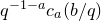


4.4 Eichler integrals of Maaß cusp forms
Proof of Corollary 1.11. For simplicity, we assume u is even or odd and let
 $j\in\{0,1\}$
be such that
$j\in\{0,1\}$
be such that
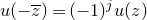 $u(-\overline z)=(-1)^ju(z)$
. The case where u is neither is believed not to be possible, but it could also be handled easily by splitting u into its even or odd components. In [Reference BruggemanBru07], it is shown that the map
$u(-\overline z)=(-1)^ju(z)$
. The case where u is neither is believed not to be possible, but it could also be handled easily by splitting u into its even or odd components. In [Reference BruggemanBru07], it is shown that the map
 $\widetilde u$
defined in (1.11) is a quantum modular form of weight 2s, whose associated period function h is defined byFootnote
11
$\widetilde u$
defined in (1.11) is a quantum modular form of weight 2s, whose associated period function h is defined byFootnote
11
 \begin{align*} h(x) = c(s)\textrm{sgn}(x)^{1-j}\psi(|x|) \quad (x\in\mathbb{R}_{\neq0}),\end{align*}
and by continuity at
 $x=0$
, where
$x=0$
, where
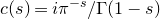 $c(s) = i \pi^{-s} / \Gamma(1-s)$
is a non-zero proportionality constant [Reference Lewis and ZagierLZ01, Equation (1.12)]. The map h is real-analytic separately on
$c(s) = i \pi^{-s} / \Gamma(1-s)$
is a non-zero proportionality constant [Reference Lewis and ZagierLZ01, Equation (1.12)]. The map h is real-analytic separately on
 $\mathbb{R}_{\leqslant 0}$
and
$\mathbb{R}_{\leqslant 0}$
and
 $\mathbb{R}_{\geqslant 0}$
and is
$\mathbb{R}_{\geqslant 0}$
and is
 $\mathcal C^{\infty}$
on
$\mathcal C^{\infty}$
on
 $\mathbb{R}$
. Thus, Theorem 1.4 applies and yields the first part of Corollary 1.11. The expansion of
$\mathbb{R}$
. Thus, Theorem 1.4 applies and yields the first part of Corollary 1.11. The expansion of
 $\psi$
at 0 is implicit in [Reference Lewis and ZagierLZ01] and can be immediately deduced by shifting the line of integration to the left in the first display of [Reference Lewis and ZagierLZ01, p. 205], from which one deduces that h(x) is not identically zero on
$\psi$
at 0 is implicit in [Reference Lewis and ZagierLZ01] and can be immediately deduced by shifting the line of integration to the left in the first display of [Reference Lewis and ZagierLZ01, p. 205], from which one deduces that h(x) is not identically zero on
 $[-1,1]$
. Thus, since the weight is
$[-1,1]$
. Thus, since the weight is
 $2s\notin\mathbb{R}$
, Theorem 3.5 applies in the case (1*), and we deduce that
$2s\notin\mathbb{R}$
, Theorem 3.5 applies in the case (1*), and we deduce that
 $(\phi\circ \widetilde u^\triangleright)_\ast(\nu)$
is diffuse. This concludes the proof of Corollary 1.11.
$(\phi\circ \widetilde u^\triangleright)_\ast(\nu)$
is diffuse. This concludes the proof of Corollary 1.11.
Remark 4.3. By the functional equation for twists of Maaß-form L-functions, [Reference Kowalski, Michel and VanderKamKMV02, (A.12) and (A.13)], we have
 $$ \widetilde u(\overline{a}/q) = q^{2s} \sum_{n\geqslant 1} \frac{a_n}{n^{1/2+s}}(c_1 \cos(2\pi n a/q) + c_2 \sin(2\pi n a/q)) \quad (a\overline a\equiv 1\pmod{q}), $$
where
 $c_1, c_2$
are numbers depending on u. With this formulation, the regularity of
$c_1, c_2$
are numbers depending on u. With this formulation, the regularity of
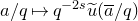 $a/q \mapsto q^{-2s} \widetilde u(\overline{a}/q)$
relates to the differentiability properties for
$a/q \mapsto q^{-2s} \widetilde u(\overline{a}/q)$
relates to the differentiability properties for
 $\widetilde g$
which we mentioned in § 1.3.1.
$\widetilde g$
which we mentioned in § 1.3.1.
An important classical problem is the analogous question when
 $a_n = d(n)$
is the divisor function, see [Reference RiemannRie68, Reference ChowlaCho31, Reference WintnerWin37]. This can be seen as the case when u is replaced by a certain weight- 0, real-analytic, non-cuspidal Eisenstein series [Reference IwaniecIwa02, p. 62]. Regularity in this case can be studied from the expression above as a Fourier series; recent general results can be found in [Reference Chamizo, Petrykiewicz and Ruiz-CabelloCPRC17].
$a_n = d(n)$
is the divisor function, see [Reference RiemannRie68, Reference ChowlaCho31, Reference WintnerWin37]. This can be seen as the case when u is replaced by a certain weight- 0, real-analytic, non-cuspidal Eisenstein series [Reference IwaniecIwa02, p. 62]. Regularity in this case can be studied from the expression above as a Fourier series; recent general results can be found in [Reference Chamizo, Petrykiewicz and Ruiz-CabelloCPRC17].
Acknowledgements
The authors are grateful to the anonymous referees and to DIMA (University of Genova) and I2M (University of Aix-Marseille), where this work was carried out, for their hospitality.
Conflicts of interest
None.
Financial support
This work has benefited from support from Aix-Marseille Université FIR Invités; from INdAM group GNAMPA; and from FWF-ANR project Arithrand: FWF: I 4945-N and ANR-20-CE91-0006. The work of the first author is partially supported by PRIN 2022 ‘The arithmetic of motives and L-functions’.
Journal information
Compositio Mathematica is owned by the Foundation Compositio Mathematica and published by the London Mathematical Society in partnership with Cambridge University Press. All surplus income from the publication of Compositio Mathematica is returned to mathematics and higher education through the charitable activities of the Foundation, the London Mathematical Society and Cambridge University Press.


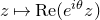


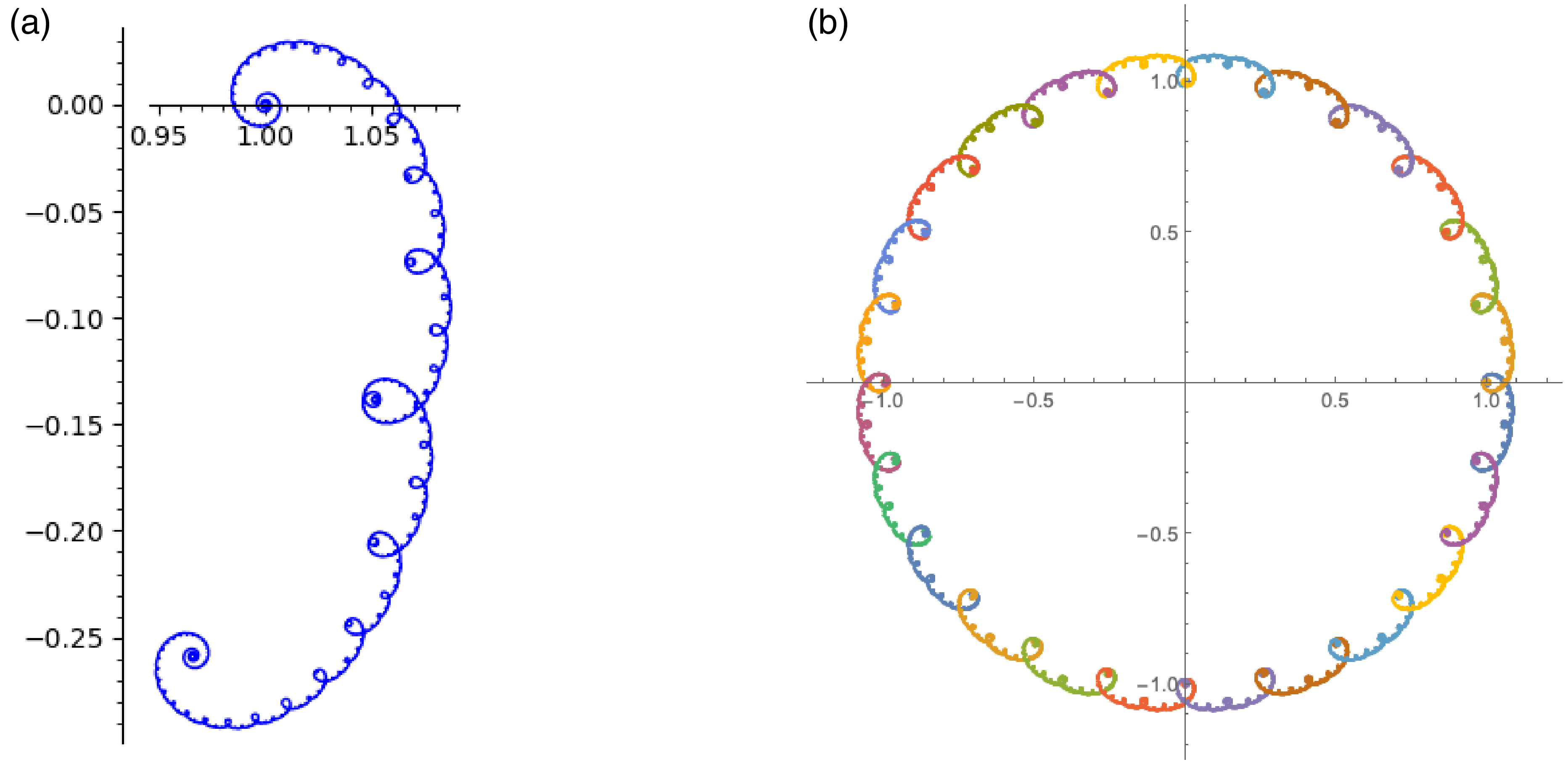


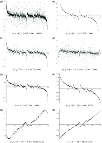


 Open access