


1. Introduction
Statistical distributions are instrumental in describing real-world phenomena across various disciplines. Despite the development of numerous distributions in actuarial and statistical literature, the complexity of real-world data – particularly in capturing rare, high-impact events, necessitates the development of flexible models to accurately model heavy-tail behavior in loss payment data. The Pareto distribution, widely regarded as a benchmark in this context, has been extensively applied (see, e.g., Johnson et al., Reference Johnson, Kotz and Balakrishnan1994; Arnold, Reference Arnold2015). However, its limitations in the upper tail area reduce its practical applicability for extreme losses. To address these shortcomings, various generalizations and extensions of the Pareto distribution have been proposed, such as the generalized Pareto distribution (GPD) introduced by Pickands (Reference Pickands1975) to improve the fitting of data. The GPD has proven effective for analyzing extreme events and modeling large insurance claims (see, e.g., Hosking and Wallis, Reference Hosking and Wallis1987; McNeil et al., Reference McNeil, Frey and Embrechts2015). Gupta et al. (Reference Gupta, Gupta and Gupta1998) introduced the exponentiated Pareto distribution and demonstrated its effectiveness in analyzing various lifetime datasets. Akinsete et al. (Reference Akinsete, Famoye and Lee2008) extended the Pareto distribution by adding two extra shape parameters based on the beta-G class of distributions introduced by Eugene et al. (Reference Eugene, Lee and Famoye2002). Based on the T-X family of distributions, Alzaatreh et al. (Reference Alzaatreh, Famoye and Lee2013) introduced and studied Weibull-Pareto distribution. Composite models have also been introduced as an alternative approach for modeling heavy-tailed data in the literature (Cooray and Ananda, Reference Cooray and Ananda2005; Nadarajah and Bakar, Reference Nadarajah and Bakar2014; Bakar et al., Reference Bakar, Hamzah, Maghsoudi and Nadarajah2015, and references therein).
The Norwegian fire insurance claims data serve as a well-known dataset where heavy-tailed models such as the GPD have been extensively analyzed. This dataset comprises fire insurance claims exceeding 500,000 Norwegian krones, recorded for the years 1972–1992 as described in Beirlant et al. (Reference Beirlant, Teugels and Vynckier1996). Initial studies by Brazauskas and Kleefeld (Reference Brazauskas and Kleefeld2011) fitted the log-folded-normal and log-folded-t distributions to the rescaled and log-transformed (thus, taking the logarithm of the data divided by 500) Norwegian claims data for the year 1988 and observed that log-folded-
 $t_7$
distribution provides a better fit than any of the competing models under consideration. Furthermore, Brazauskas and Kleefeld (Reference Brazauskas and Kleefeld2016) fitted truncated versions of the GPD and other alternative models to the Norwegian fire insurance claims data. Later, Mdziniso and Cooray (Reference Mdziniso and Cooray2018) introduced the odd Pareto distribution, derived from the odds of the Pareto and inverse Pareto distributions, and fitted it to analyze the Norwegian fire insurance claims datasets for 1988 and 1990, respectively. Most recently, Aljadani (Reference Aljadani2024) used Norwegian fire insurance claims data to demonstrate the effectiveness of the
$t_7$
distribution provides a better fit than any of the competing models under consideration. Furthermore, Brazauskas and Kleefeld (Reference Brazauskas and Kleefeld2016) fitted truncated versions of the GPD and other alternative models to the Norwegian fire insurance claims data. Later, Mdziniso and Cooray (Reference Mdziniso and Cooray2018) introduced the odd Pareto distribution, derived from the odds of the Pareto and inverse Pareto distributions, and fitted it to analyze the Norwegian fire insurance claims datasets for 1988 and 1990, respectively. Most recently, Aljadani (Reference Aljadani2024) used Norwegian fire insurance claims data to demonstrate the effectiveness of the
 $\text{PORT-VAR}_q$
method in risk analysis. Considering the recommendation of Scollnik (Reference Scollnik2014), we analyze the complete Norwegian fire insurance claims data from 1972 to 1992 without transforming or scaling the original values.
$\text{PORT-VAR}_q$
method in risk analysis. Considering the recommendation of Scollnik (Reference Scollnik2014), we analyze the complete Norwegian fire insurance claims data from 1972 to 1992 without transforming or scaling the original values.
The log-logistic (LL) distribution, also known as the Fisk distribution and commonly used to model income distributions, is sometimes referred to as Pareto Type III distribution. The LL distribution provides a valuable model due to its versatility in claim size modeling. In particular, researchers assume that smaller claims follow standard distributions such as log-normal, LL or Weibull, while larger claims are better modeled using a Pareto-type distribution (Brazauskas and Kleefeld, Reference Brazauskas and Kleefeld2016). Studies by Scollnik (Reference Scollnik2007) and Scollnik and Sun (Reference Scollnik and Sun2012) demonstrate that modeling large claims using a Pareto-type distribution yields promising results.
In practice, claim size data are often truncated, where observations are restricted to specific ranges due to policy limits, deductibles, or reporting thresholds. Recognizing the importance of generalized families of distributions and the practical relevance of truncation in modeling, we introduce a novel family of distributions developed under theoretical framework called Enriched Truncated Exponentiated Generalized family (ETE-G).
Let
 $g(x;\,\boldsymbol{\Omega})$
and
$g(x;\,\boldsymbol{\Omega})$
and
 $G(x;\,\boldsymbol{\Omega})$
denote the pdf and cdf of the baseline distribution with parameter vector
$G(x;\,\boldsymbol{\Omega})$
denote the pdf and cdf of the baseline distribution with parameter vector
 $\boldsymbol{\Omega}$
and support
$\boldsymbol{\Omega}$
and support
 $\mathcal{S_G}$
. For notational simplicity, we omit
$\mathcal{S_G}$
. For notational simplicity, we omit
 $\boldsymbol{\Omega}$
and write
$\boldsymbol{\Omega}$
and write
 $G(x)=G(x;\,\boldsymbol{\Omega})$
and
$G(x)=G(x;\,\boldsymbol{\Omega})$
and
 $g(x)=g(x;\,\boldsymbol{\Omega}).$
We define the Exponentiated-G family introduced by Gupta et al. (Reference Gupta, Gupta and Gupta1998) through a power transformation on a baseline cdf G(x) as follows:
$g(x)=g(x;\,\boldsymbol{\Omega}).$
We define the Exponentiated-G family introduced by Gupta et al. (Reference Gupta, Gupta and Gupta1998) through a power transformation on a baseline cdf G(x) as follows:
 \begin{align} F(x) = [G(x)]^a,\qquad \text{and} \qquad f(x) = ag(x)(G(x))^{a-1}, \quad a\gt0 , x \in \mathcal{S_G}.\end{align}
Suppose the baseline distribution is truncated at a threshold
 $W(\theta_0),$
where
$W(\theta_0),$
where
 $W(\theta_0)$
is a function of a scale parameter
$W(\theta_0)$
is a function of a scale parameter
 $\theta_0$
of G(x). The resulting truncated Exp–G distribution has cdf and pdf
$\theta_0$
of G(x). The resulting truncated Exp–G distribution has cdf and pdf
 \begin{align}F(x) = \dfrac{[G(x)]^a - [G(W(\theta_0))]^a}{1 - [G(W(\theta_0))]^a},\quad \text{and} \quad f(x)= \frac{a g(x)[G(x)]^{a-1}}{1 - [G(W(\theta_0))]^{a}},\quad a\gt0, x\gt\theta_0.\end{align}
For computational convenience in parameter estimation, we assume
 $W(\theta_0)$
corresponds to the median of G(x). For example, if the baseline distribution is Weibull,
$W(\theta_0)$
corresponds to the median of G(x). For example, if the baseline distribution is Weibull,
 $G(x) = 1-\exp[{-}(x/\theta)^\alpha]$
, the median is
$G(x) = 1-\exp[{-}(x/\theta)^\alpha]$
, the median is
 $\theta (\!\ln 2)^{1/\alpha}$
, with support
$\theta (\!\ln 2)^{1/\alpha}$
, with support
 $x\gt\theta_0(\!\ln 2)^{1/\alpha}$
. However, maximum likelihood estimation can become cumbersome because the first-order statistic for the truncated distribution from (1.2) may involve functional form other than
$x\gt\theta_0(\!\ln 2)^{1/\alpha}$
. However, maximum likelihood estimation can become cumbersome because the first-order statistic for the truncated distribution from (1.2) may involve functional form other than
 $\theta_0$
, complicating the likelihood. In contrast, for a LL distribution in log-location form,
$\theta_0$
, complicating the likelihood. In contrast, for a LL distribution in log-location form,
 $G(x) = [1 + e^{-(\!\log x - \theta)/\sigma}]^{-1}$
, the median is
$G(x) = [1 + e^{-(\!\log x - \theta)/\sigma}]^{-1}$
, the median is
 $e^{\theta}$
, yielding support
$e^{\theta}$
, yielding support
 $x\gt e^{\theta_0}$
. Therefore,
$x\gt e^{\theta_0}$
. Therefore,
 $W(\theta_0)$
must depend solely on the scale parameter of the baseline distribution. To enhance both interpretability and analytical tractability, we therefore center the truncation at the median of G(x), ensuring the transformation is anchored at a meaningful reference point.
$W(\theta_0)$
must depend solely on the scale parameter of the baseline distribution. To enhance both interpretability and analytical tractability, we therefore center the truncation at the median of G(x), ensuring the transformation is anchored at a meaningful reference point.
In a more general setting, one may consider truncation at an arbitrary reference point
 $\theta_0$
(with
$\theta_0$
(with
 $W(\theta_0)=\theta_0$
as in this paper), in which case Equation (1.2) reduces to
$W(\theta_0)=\theta_0$
as in this paper), in which case Equation (1.2) reduces to
 \begin{align*} F(x) = \dfrac{[G(x)]^a - \gamma^{-a}}{1 - \gamma^{-a}}, \end{align*}
where
 $G(x) \rightarrow \frac{1}{\gamma}$
as
$G(x) \rightarrow \frac{1}{\gamma}$
as
 $x \rightarrow W(\theta_0)$
for some
$x \rightarrow W(\theta_0)$
for some
 $\gamma\gt1$
. In practice, however, this generalization often leads to convergence and identifiability issues, so we restrict truncation at the median. As a result,
$\gamma\gt1$
. In practice, however, this generalization often leads to convergence and identifiability issues, so we restrict truncation at the median. As a result,
 $W(\theta_0)$
should satisfy
$W(\theta_0)$
should satisfy
 $G(x) \to \tfrac{1}{2}$
as
$G(x) \to \tfrac{1}{2}$
as
 $x \to W(\theta_0).$
It follows that the truncated Exp–G distribution simplifies to
$x \to W(\theta_0).$
It follows that the truncated Exp–G distribution simplifies to
 \begin{align}F(x) &= \dfrac{[G(x)]^a - 2^{-a}}{1 - 2^{-a}}, \qquad a\gt0, \; x\gt\theta,\end{align}
which may be enriched by reparameterizing a as
 $\beta=\pm a$
with
$\beta=\pm a$
with
 $a\gt0$
, yielding the proposed ETE-G cdf and pdf:
$a\gt0$
, yielding the proposed ETE-G cdf and pdf:
 \begin{align} F(x) = \dfrac{ 2^{\beta} - {(G(x))^{-\beta}} }{2^{\beta} -1};\,\quad x\gt\theta, \ -\infty \lt \beta \lt \infty, \ \beta \neq 0 , \\[-30pt] \nonumber \end{align}
 \begin{align} f(x) =\dfrac{\beta g(x){(G(x))^{-(\beta+1)}}}{2^{\beta} -1},\quad x\gt\theta, \ -\infty \lt \beta \lt \infty, \ \beta \neq 0. \\[5pt] \nonumber \end{align}
where
 $\beta$
is a parameter that reflects the enriched nature of the ETE-G family. It can take either positive or negative values, allowing the distribution to adapt to a wide density and hazard shapes. G(x) also serves as the cdf of the baseline distribution and must satisfy
$\beta$
is a parameter that reflects the enriched nature of the ETE-G family. It can take either positive or negative values, allowing the distribution to adapt to a wide density and hazard shapes. G(x) also serves as the cdf of the baseline distribution and must satisfy
-
(i)
 $G(x) \rightarrow \frac{1}{2}$
as
$x \rightarrow \theta$
, where
$\theta$
is the median of
$G(x).$
$G(x) \rightarrow \frac{1}{2}$
as
$x \rightarrow \theta$
, where
$\theta$
is the median of
$G(x).$


The parameter
 $\theta$
is assumed to be known and can be interpreted as the deductible or threshold of the ETE-G family, analogous to the threshold parameter in the Pareto distribution. Clearly, Equation (1.4) provides a tool for obtaining a parametric distribution from an existing one.
$\theta$
is assumed to be known and can be interpreted as the deductible or threshold of the ETE-G family, analogous to the threshold parameter in the Pareto distribution. Clearly, Equation (1.4) provides a tool for obtaining a parametric distribution from an existing one.
The corresponding hazard (or failure rate) function is given by
 \begin{equation} h(x) =\dfrac{\beta g(x){(G(x))^{-(\beta+1)}}}{{(G(x))^{-\beta}}-1},\quad x\gt\theta, \ -\infty \lt \beta \lt\infty, \ \beta \neq 0.\end{equation}
Furthermore, the quantile function of ETE-G family takes the following form:
 \begin{equation} Q(u) =G^{-1}\left[ 2^{\beta} - u(2^{\beta} - 1)\right]^{-1/\beta}, \quad 0 \le u \le 1,\end{equation}
where
 $G^{-1}(.)$
is the baseline quantile function.
$G^{-1}(.)$
is the baseline quantile function.
Among the sub-models within ETE-G family, we will introduce and develop a new three-parameter sub-model derived from the LL distribution having a flexible upper tail in modeling loss payment data. This distribution, detailed in Section 2 will be referred to as the Enriched Truncated Exponentiated Log-logistic (ETELL) distribution, as it is constructed by enriching a truncated exponentiated LL distribution. The main motivations of the ETE-G family are (i) to obtain a more flexible model with fewer parameters and achieve better goodness-of-fit on the real insurance data, (ii) to generate various types of distributional shapes, (iii) to build heavy-tailed distributions for modeling real data, and (iv) to provide consistently better fits than other generated models under the same baseline distribution.
The outline of this article is as follows. In Section 2, we define the ETELL distribution, present some special cases, and explore its distributional properties. Some of these properties are the quantiles, the mean, a discussion on the moments of the distribution, and Shannon entropy for ETELL distribution. The tail behavior and tail heaviness properties are discussed in Section 3. In Section 4.1, we provide maximum likelihood (ml) estimators of the parameters of the ETELL distribution and the uniqueness of the estimates. Section 4.2 includes elements of the Fisher information matrix for the ETELL distribution. Some other members of the ETE-G family of distributions are discussed in Section 5. The ETE-G family of distributions are fitted to the Norwegian fire insurance claim dataset, and the results are presented in Section 6. Section 6.1 discusses the application of these models to risk measures and describes an empirical backtesting procedure to validate these measures. Finally, in Section 7, we conclude with some remarks on the main results and their significance.
2. Enriched truncated exponentiated log-logistic distribution
Let X be a LL random variable, then the cumulative distribution function of X is defined as
 \begin{equation} G(x) =\dfrac{1}{\left[1+\left(\frac{\theta}{x}\right)^\alpha\right]}, \quad x\gt0, \alpha\gt0,\end{equation}
where
 $\theta\gt0$
is the scale parameter and also represent the median of the distribution,
$\theta\gt0$
is the scale parameter and also represent the median of the distribution,
 $\alpha\gt0$
is the shape parameter and the distribution is unimodal when
$\alpha\gt0$
is the shape parameter and the distribution is unimodal when
 $\alpha\gt1.$
Using (1.4), the cdf of ETELL distribution is expressed as
$\alpha\gt1.$
Using (1.4), the cdf of ETELL distribution is expressed as
 \begin{equation}F(x,\alpha,\beta,\theta)=\begin{cases}\dfrac{2^\beta-\left[1+\left(\frac{\theta}{x}\right)^\alpha\right]^\beta}{2^\beta-1}, & \beta \neq 0 , \ x \geq\theta, \alpha\gt0 \\&\\1-\dfrac{\ln \left[1+\left(\frac{\theta}{x}\right)^\alpha\right]}{\ln 2},& \beta = 0 , \ x \geq \theta, \alpha\gt0\end{cases}\end{equation}
The corresponding probability density function to (2.2) is given by
 \begin{equation}f(x;\,\alpha,\beta,\theta)=\begin{cases}\dfrac{{\alpha}{\beta}}{\left(2^{\beta}-1\right)x}\left(\dfrac{{\theta}}{x}\right)^{\alpha}\left[1+\left(\dfrac{\theta}{x}\right)^\alpha\right]^{\beta-1}, & \beta \neq 0, \ x \geq \theta, \alpha\gt0 \\&\\\dfrac{\alpha}{x\ln2 }\left(\dfrac{{\theta}}{x}\right)^{\alpha}\left[1+\left(\dfrac{\theta}{x}\right)^\alpha\right]^{-1},& \beta = 0 , \ x \geq \theta, \alpha\gt0\end{cases}\end{equation}
where
 $ -\infty \lt \beta \lt \infty $
and
$ -\infty \lt \beta \lt \infty $
and
 $ \alpha \gt 0 $
are shape parameters, and
$ \alpha \gt 0 $
are shape parameters, and
 $ \theta \gt 0 $
is the scale parameter. Subsequently, we denote a random variable X following the density in (2.3) by
$ \theta \gt 0 $
is the scale parameter. Subsequently, we denote a random variable X following the density in (2.3) by
 $ X \sim \text{ETELL}(\alpha, \beta, \theta) $
. We note that, although the ETELL distribution and the shifted log-logistic (SLL) distribution both have support
$ X \sim \text{ETELL}(\alpha, \beta, \theta) $
. We note that, although the ETELL distribution and the shifted log-logistic (SLL) distribution both have support
 $(\theta, \infty)$
, the ETELL is distinct and offers greater flexibility. In particular, the Pareto distribution is embedded as a special case of the ETELL when
$(\theta, \infty)$
, the ETELL is distinct and offers greater flexibility. In particular, the Pareto distribution is embedded as a special case of the ETELL when
 $\beta = 1$
, a structural property that distinguishes it from the SLL. Furthermore, the ETELL is heavy-tailed, as discussed in Section 3, whereas the SLL does not exhibit heavy-tailed behavior.
$\beta = 1$
, a structural property that distinguishes it from the SLL. Furthermore, the ETELL is heavy-tailed, as discussed in Section 3, whereas the SLL does not exhibit heavy-tailed behavior.
Considering a random variable X that follows the ETELL distribution, the survival function S(x) and the hazard rate function (or failure rate) are defined, respectively, as
 \begin{align*} S(x) =1 -F(x) = \dfrac{\left[ 1+\left(\frac{\theta}{x}\right)^\alpha\right]^\beta-1}{2^\beta-1} \end{align*}
 \begin{align*} h(x) =\dfrac{f(x)}{S(x)} = \dfrac{\alpha \beta }{x} \left(\dfrac{\theta}{x} \right)^\alpha\frac{\left[ 1+\left(\frac{\theta}{x} \right)^\alpha\right]^{\beta-1}}{\left[1+\left(\frac{\theta}{x}\right)^\alpha\right]^\beta-1} \end{align*}
where F(x) and f(x) are given by (2.2) and (2.3), respectively.
2.1. Special cases
We consider the following special cases of the ETELL distribution, which correspond to known distributions:
-
(a) When
$\beta=1$
, the ETELL distribution in (2.2) reduces to the Pareto distribution. -
(b) When
$\beta=-1$
, the ETELL distribution in (2.2) reduces to a new Pareto distribution by Bourguignon et al. (Reference Bourguignon, Saulo and Fernandez2016), with cdf
\begin{align*} F(x) = \dfrac{1-\left(\frac{\theta}{x}\right)^\alpha}{1+\left(\frac{\theta}{x}\right)^\alpha}=1-\dfrac{2\left( \frac{\theta}{x}\right)^\alpha}{1+\left(\frac{\theta}{x}\right)^\alpha} , \quad x\geq \theta, \alpha\gt0.\end{align*}


2.2. Distributional properties
The quantile function of the ETELL distribution, say
 $x=Q(u)$
, can easily be obtained as
$x=Q(u)$
, can easily be obtained as
 \begin{equation} x=Q(u)=F^{-1}(u)=\theta \left\{\left[2^\beta -(2^\beta -1)u\right]^{\frac{1}{\beta}}-1\right\}^{-\frac{1}{\alpha}}, \quad 0 \lt u\lt 1.\end{equation}
We compute the median of the ETELL distribution as follows, we set
 $F(x;\,\alpha,\beta,\theta)=0.5$
in (2.2) and solve for x,
$F(x;\,\alpha,\beta,\theta)=0.5$
in (2.2) and solve for x,
 \begin{align*} \therefore \ \text{Median}(X) =\theta\left[ \left(\dfrac{2^\beta+1}{2}\right)^ \frac{1}{\beta} - 1 \right]^{-\frac{1}{\alpha}}. \end{align*}
The first and third quartiles,
 $Q(1/4)$
and
$Q(1/4)$
and
 $Q(3/4),$
can be obtained by setting
$Q(3/4),$
can be obtained by setting
 $u=0.25$
and
$u=0.25$
and
 $u=0.75$
into (2.4), respectively.
$u=0.75$
into (2.4), respectively.
Theorem 2.1 (Unimodality).
The ETELL distribution is unimodal when
 $\beta\lt -\frac{1}{\alpha}$
, with mode at
$\beta\lt -\frac{1}{\alpha}$
, with mode at
 \begin{align*} x_0 = \theta \left[ -\dfrac{(1+\alpha\beta)}{(1+\alpha)}\right]^{\frac{1}{\alpha}}. \end{align*}
Proof. Taking the derivative of the pdf in (2.3), we obtain
 \begin{equation} f^\prime(x)=-\dfrac{\alpha\beta}{(2^\beta-1)x^2}\left( \dfrac{\theta}{x}\right)^\alpha\left[ 1+\left(\frac{\theta}{x}\right)^\alpha\right]^{\beta-2}\left\{1+\alpha+\left(1+\alpha\beta\right)\left( \frac{\theta}{x}\right)^\alpha \right\}. \end{equation}
Setting
 $ f^\prime(x) = 0 $
, the critical point occurs at
$ f^\prime(x) = 0 $
, the critical point occurs at
 \begin{equation}{} x_0 = \theta \left[{-} \dfrac{(1+\alpha\beta)}{(1+\alpha)}\right]^{\frac{1}{\alpha}}\end{equation}
Since
 $x\geq \theta$
and
$x\geq \theta$
and
 $\alpha\gt0$
, it is necessary that
$\alpha\gt0$
, it is necessary that
 $-(1+\alpha\beta) \geq 0$
implying that
$-(1+\alpha\beta) \geq 0$
implying that
 $\beta\lt -\frac{1}{\alpha}.$
For
$\beta\lt -\frac{1}{\alpha}.$
For
 $\beta \ge -\frac{1}{\alpha}$
, then ETELL distribution is a decreasing function of x and its maximum is at the point
$\beta \ge -\frac{1}{\alpha}$
, then ETELL distribution is a decreasing function of x and its maximum is at the point
 $x_0=\theta$
.
$x_0=\theta$
.
Lastly,
 \begin{align*}f^{\prime \prime}(x_0)=\dfrac{\alpha^2\beta(1+\alpha\beta)}{(2^\beta-1)x_0^3}\left( \dfrac{\theta}{x_0}\right)^{2\alpha} \left[ 1+\left( \dfrac{\theta}{x_0}\right)^{\alpha}\right]^{\beta-2}\lt 0, \ \quad \beta\lt-\frac{1}{\alpha}.\end{align*}
Thus
 $x_0$
in (2.6) is a global maximum. This concludes the proof.
$x_0$
in (2.6) is a global maximum. This concludes the proof.
The shape of the density described in Theorem (2.1) and the corresponding hazard rate functions of the ETELL distribution are illustrated in Figure 1. The density can exhibit various shapes, including symmetrical, right-skewed, or reverse-J shapes, while the hazard rate exhibits both decreasing and upside-down bathtub shapes.

Figure 1. ETE-G sub-models – densities (left panel) and hazard functions (right panel). From top to bottom: ETELL (top-left two plots), ETEPC (top-right two plots), ETELN (middle-left two plots), ETELC (middle-right two plots), EETEFC (bottom-left two plots), and ETEBS (bottom-right two plots). Each pair of plots illustrates the density and hazard behavior under different parameter settings.
2.3. Limit behavior
Lemma 1. The limit of ETELL density function and hazard function as
 $x \rightarrow \theta $
is given by
$x \rightarrow \theta $
is given by
 \begin{equation*} \lim_{x \rightarrow \theta } f(x;\,\alpha, \beta, \theta) = \lim_{x \rightarrow \theta } h(x;\,\alpha, \beta, \theta)=\begin{cases} \left(\dfrac{\alpha \beta}{\theta} \right)\left( \dfrac{2^{\beta-1}}{2^\beta-1}\right) , & \text{for} \ \beta \neq 0\\[12pt] \dfrac{\alpha}{2\theta \ln 2}, & \text{for} \ \beta=0 \end{cases}\end{equation*}
Lemma 2. The limit of the ETELL density function and hazard function as
 $x \rightarrow\infty$
is 0
$x \rightarrow\infty$
is 0
2.4. Moment function of ETELL
Let X denote a random variable that follows the ETELL distribution. Then, the moment generating function of
 $(X/\theta)^k$
is given by
$(X/\theta)^k$
is given by
 \begin{align}\mathbb{E} \left(\dfrac{X}{\theta} \right)^k & =\int_\theta^{\infty} \frac{a \beta}{\left(2^\beta-1\right) x}\left(\frac{x}{\theta}\right)^{k-\alpha}\left[1+\left(\frac{\theta}{x}\right)^\alpha\right]^{\beta-1} d x, \quad \text{Let} \left(\dfrac{\theta}{x}\right)^\alpha=t, \notag\\& =\int_0^1 \frac{\beta}{2^\beta-1} t^{-\frac{k}{\alpha}}(1+t)^{\beta-1} d t.\end{align}
Making an appropriate adjustment of (2.7), the kth moment of ETELL distribution can be expressed as
 \begin{align}\mathbb{E}(X^k)&=\left\{\begin{array}{l}\dfrac{\theta^k\beta}{2^\beta-1} \mathop{\sum}\limits_{r=0}^{{\beta-1}}\left(\begin{array}{c}\beta-1 \\ r\end{array}\right) \dfrac{1}{(1+r)-\frac{k}{\alpha}}, \text { if } \ \beta \in \mathbb{Z}^{+}\setminus\{1\}, \ 1+r \gt \frac{k}{\alpha}, \ k \lt \alpha \\[17pt] \dfrac{\theta^k \beta}{2^\beta-1} \mathop{\sum}\limits_{r=0}^{\infty}\left(\begin{array}{c}\beta-1 \\r\end{array}\right) \dfrac{1}{1+r-\frac{k}{\alpha}}, \text { if } \ \beta \notin \mathbb{Z}^{+}, \ 1+r \gt \frac{k}{\alpha} , \ k \lt \alpha\end{array}\right.\end{align}
where
 $\mathbb{Z}^+$
is a positive set. When
$\mathbb{Z}^+$
is a positive set. When
 $k=1$
in (2.8), we get the mean of the ETELL distribution.
$k=1$
in (2.8), we get the mean of the ETELL distribution.
In particular, for
 $\beta=k=1$
, (2.8) reduces to:
$\beta=k=1$
, (2.8) reduces to:
 \begin{align*}\mu=\mathbb{E}(X)= \dfrac{\alpha \theta}{\alpha -1 }, \quad \alpha\gt0\end{align*}
which is the mean of Pareto distribution.
2.5. Shannon entropy
The Shannon entropy of a random variable X is a measure of the variation or uncertainty in its distribution. For a continuous random variable X, the Shannon entropy, as defined by Shannon (Reference Shannon1948), is given by
 \begin{align*}H(X)=\mathbb{E}[{-}ln(f(x))] = -\int_\theta^\infty \ln f(x) f(x) dx.\end{align*}
By using ETELL density, we have
 \begin{align*} H(X)=-\ln\left[\frac{\alpha \beta}{\theta(2^\beta-1)}\right] -\dfrac{(\alpha+1)\beta I_{\mathcal{B}-1}}{\alpha(2^\beta-1)} -\dfrac{(\beta-1)(\beta \cdot 2^\beta\ln2-2^\beta+1)}{\beta(2^\beta-1)},\end{align*}
where
 $I_{\mathcal{B}-1}$
is defined in Equation (4.5). The detailed derivation is provided in Appendix A.
$I_{\mathcal{B}-1}$
is defined in Equation (4.5). The detailed derivation is provided in Appendix A.
3. Tail behavior
Heavy-tailed distributions play an important role in applications where extreme values significantly influence overall outcomes, such as fire and catastrophe insurance, genetics, and environmental extremes (Klugman et al., Reference Klugman, Panjer and Willmot2012). In this section, we outline several criteria used to assess the heaviness of a distribution’s tail.
A widely used criterion for assessing tail heaviness is based on regular variation. A distribution with cdf F is said to have a heavy tail whenever the survival function,
 $\overline{F}(x) =1-F(x)=P(X\gt x)$
, regularly varies at infinity with a negative index of regular variation,
$\overline{F}(x) =1-F(x)=P(X\gt x)$
, regularly varies at infinity with a negative index of regular variation,
 $-1/\xi$
, where
$-1/\xi$
, where
 $\xi\gt0$
(see, e.g., Gnedenko, Reference Gnedenko1943; Gnedenko and Kolmogorov, Reference Gnedenko and Kolmogorov1968). Thus, for every
$\xi\gt0$
(see, e.g., Gnedenko, Reference Gnedenko1943; Gnedenko and Kolmogorov, Reference Gnedenko and Kolmogorov1968). Thus, for every
 $x\gt0$
,
$x\gt0$
,
 \begin{equation} \lim\limits_{t \rightarrow \infty } \dfrac{ \overline{F}(tx)}{\overline{F} (t)} = x^{-1/\xi} \ \ \ \text{(Right tail)}\end{equation}
The parameter
 $\xi$
is known as the tail index, which governs the rate of decay in the tails. Whenever
$\xi$
is known as the tail index, which governs the rate of decay in the tails. Whenever
 $\xi \rightarrow 0$
, we say that the distribution F(x) has a light (non-heavy) right tail. And whenever
$\xi \rightarrow 0$
, we say that the distribution F(x) has a light (non-heavy) right tail. And whenever
 $\xi \rightarrow \infty$
, the distribution F(x) has a heavy right tail. Using the cdf of ETELL in (2.2), (3.1) may be expressed as
$\xi \rightarrow \infty$
, the distribution F(x) has a heavy right tail. Using the cdf of ETELL in (2.2), (3.1) may be expressed as
 \begin{equation*} \lim\limits_{t\to \infty} \dfrac{\overline{F}(tx)}{\overline{F} (t)} = \lim\limits_{t\to \infty} \dfrac{\left[1+\left( \frac{\theta}{tx}\right)^\alpha\right]^\beta-1}{\left[1+\left( \frac{\theta}{t}\right)^\alpha\right]^\beta-1} =x^{-1/(\frac{1}{\alpha})}.\end{equation*}
Thus, the ETELL distribution has a heavy right tail with a tail index
 $\xi=1/\alpha$
. As
$\xi=1/\alpha$
. As
 $\alpha \rightarrow 0,$
the distribution becomes increasingly heavy-tailed, and as
$\alpha \rightarrow 0,$
the distribution becomes increasingly heavy-tailed, and as
 $\alpha \rightarrow \infty,$
the tail becomes light. The derivation is provided in Appendix B.
$\alpha \rightarrow \infty,$
the tail becomes light. The derivation is provided in Appendix B.
An alternative criterion considers the existence of moments. A distribution is heavy-tailed if its kth raw moment exists only for certain values of k. As shown in (2.8), the ETELL distribution has finite moments only when
 $k\lt\alpha$
, providing further evidence of its heavy-tailed behavior.
$k\lt\alpha$
, providing further evidence of its heavy-tailed behavior.
Tail heaviness can be a relative concept (distribution A has a heavier right tail than distribution B). A common approach used that one distribution has a heavier tail than another distribution with the same mean is the limit of the ratio of the survival functions:
 \begin{align} \lim\limits_{x \rightarrow \infty} \dfrac{S_1(x)}{S_2(x)} = \lim\limits_{x \rightarrow \infty}\dfrac{S^\prime_1(x)}{S^\prime_1(x)}= \lim\limits_{x \rightarrow \infty} \dfrac{f_1(x)}{f_2(x)} =\begin{cases} \infty \quad f_1(x) \ \text{has a heavier tail than } f_2(x)\\[2pt] 0 \quad \quad f_1(x) \ \text{has a lighter tail than } f_2(x). \end{cases}\end{align}
Using this criterion in (3.2), one can show that the
 $ETELL(\alpha,\beta,\theta)$
distribution has a heavier tail than the odd Pareto distribution,
$ETELL(\alpha,\beta,\theta)$
distribution has a heavier tail than the odd Pareto distribution,
 $OP(\alpha_0,\beta_0,\theta_0),$
introduced by Mdziniso and Cooray (Reference Mdziniso and Cooray2018) when
$OP(\alpha_0,\beta_0,\theta_0),$
introduced by Mdziniso and Cooray (Reference Mdziniso and Cooray2018) when
 $\alpha_0\beta_0\gt\alpha.$
Conversely, if
$\alpha_0\beta_0\gt\alpha.$
Conversely, if
 $\alpha_0\beta_0\lt\alpha,$
 $f_{ETELL}$
has a light tail. If
$f_{ETELL}$
has a light tail. If
 $\alpha_0\beta_0 = \alpha,$
the tails are of comparable heaviness. See Appendix C for detailed comparison.
$\alpha_0\beta_0 = \alpha,$
the tails are of comparable heaviness. See Appendix C for detailed comparison.
4. Parameter estimation
In this section, we apply ml estimation to estimate the ETELL distribution model parameters and derive the Fisher information matrix. A simulation study is also conducted to assess the performance of the ml estimators of the ETELL parameters.
4.1. Maximum likelihood estimates of parameters
In modeling a given data, understanding the model’s parameter values is important. However, in practice, these parameters are typically unknown and must be estimated from the data. In this Section, we derive the parameter estimates for the ETELL distribution using the method of ml which can help us model the data in Section 6. Let
 $X_1, X_2,\ldots, X_n$
be a complete random sample of size n, drawn from the ETELL density given in Equation (2.3). The corresponding log-likelihood function can be expressed as:
$X_1, X_2,\ldots, X_n$
be a complete random sample of size n, drawn from the ETELL density given in Equation (2.3). The corresponding log-likelihood function can be expressed as:
 \begin{equation}l(\theta)=n \ln \alpha+ n\ln \left(\frac{\beta}{2^\beta-1}\right)+n \alpha \ln \theta-(1+\alpha) \sum_{i=1}^n \ln x_i+(\beta-1) \sum_{i=1}^n \ln \left[1+\left(\frac{\theta}{x_i}\right)^\alpha\right].\end{equation}
Taking the partial derivative of (4.1) w.r.t the parameter vector
 $[\alpha, \beta]^\prime$
, we obtain the following;
$[\alpha, \beta]^\prime$
, we obtain the following;
 \begin{equation} \frac{\partial l}{\partial \alpha}=\frac{n}{\alpha}+\sum_{i=1}^n\left[\frac{1+\beta\left(\frac{\theta}{x_i}\right)^\alpha}{1+\left(\frac{\theta}{x_i}\right)^a}\right] \ln \left(\frac{\theta}{x_i}\right) , \end{equation}
 \begin{align} \frac{\partial l}{\partial \beta}=\frac{n}{\beta}- n\ln 2 \cdot \left(\frac{2^\beta}{2^\beta-1}\right) +\sum_{i=1}^n \ln \left[1+\left(\frac{\theta}{x_i}\right)^\alpha\right]. \\ \nonumber \end{align}
The ml estimators of the parameters
 $\alpha$
and
$\alpha$
and
 $\beta$
can be obtained by setting the resulting expressions to zero and solving the system of nonlinear equations. To solve these equations, the initial estimate of the parameters was set at
$\beta$
can be obtained by setting the resulting expressions to zero and solving the system of nonlinear equations. To solve these equations, the initial estimate of the parameters was set at
 $\alpha = \beta = 1$
, which runs smoothly and quickly without convergence issues. Since
$\alpha = \beta = 1$
, which runs smoothly and quickly without convergence issues. Since
 $x\geq \theta$
, the ml estimator
$x\geq \theta$
, the ml estimator
 $\hat{\theta}$
is the first-order statistic
$\hat{\theta}$
is the first-order statistic
 $x_{(1)}$
. Directly solving this system is not possible. However, the following theorem provides the existence and uniqueness of ml estimators of the ETELL distribution.
$x_{(1)}$
. Directly solving this system is not possible. However, the following theorem provides the existence and uniqueness of ml estimators of the ETELL distribution.
Theorem 4.1 (Uniqueness of ml estimators).
The ml estimators of the parameters of the ETELL distribution exist. Furthermore, they can uniquely be determined when
 $\lvert \beta \rvert \lt1.$
Proof. Let
 $\frac{\partial l}{\partial \beta}=g(\beta)=0$
from (4.3) and check the end behavior of
$\frac{\partial l}{\partial \beta}=g(\beta)=0$
from (4.3) and check the end behavior of
 $ g(\beta)$
.
$ g(\beta)$
.
 \begin{align*} g(\beta)&= \frac{n}{\beta}- n\ln 2 \cdot \left(\frac{1}{1-2^{-\beta}}\right) +\sum_{i=1}^n \ln \left[1+\left(\frac{\theta}{x_i}\right)^\alpha\right].\end{align*}
It is straightforward to verify that
 $g(\beta)$
diverges to a positive constant as
$g(\beta)$
diverges to a positive constant as
 $\beta \to -\infty$
and to a negative constant as
$\beta \to -\infty$
and to a negative constant as
 $\beta \to \infty$
. Furthermore, we check the monotonicity of
$\beta \to \infty$
. Furthermore, we check the monotonicity of
 $g(\beta)$
, with a proof given in Appendix C.
$g(\beta)$
, with a proof given in Appendix C.
 \begin{align*}g^{\prime}(\beta)=-\frac{n}{\beta^2}+\frac{2^\beta \cdot n \ln ^22}{\left(2^\beta-1\right)^2} = -\frac{n}{\beta^2\left(2^\beta-1\right)^2} \underbrace{\left[\frac{\beta^4 \ln ^4 2}{8}+\mathcal{O}(n)\right]}_{\gt 0} \lt 0. \end{align*}
This proves the existence and uniqueness of the ml estimator for
 $\beta$
whenever
$\beta$
whenever
 $\lvert \beta \rvert \le 1.$
Similarly, we set
$\lvert \beta \rvert \le 1.$
Similarly, we set
 $\frac{\partial l}{\partial \alpha} = g(\alpha)=0$
from (4.2) and check the end behavior of
$\frac{\partial l}{\partial \alpha} = g(\alpha)=0$
from (4.2) and check the end behavior of
 $ g(\alpha).$
 \begin{align*} & g(\alpha)=n+\alpha \sum_{i=1}^n\left[\frac{1+\beta\left(\frac{\theta}{x_i}\right)^\alpha}{1+\left(\frac{\theta}{x_i}\right)^\alpha}\right] \ln \left(\frac{\theta}{x_i}\right)\end{align*}
It is straightforward to verify that
 $ g(\alpha) \to n $
as
$ g(\alpha) \to n $
as
 $ \alpha \to 0^+ $
and
$ \alpha \to 0^+ $
and
 $ g(\alpha) \to -\infty $
as
$ g(\alpha) \to -\infty $
as
 $ \alpha \to \infty $
. We assess the monotonic behavior of
$ \alpha \to \infty $
. We assess the monotonic behavior of
 $g(\alpha),$
where a detailed proof is provided in Appendix D.
$g(\alpha),$
where a detailed proof is provided in Appendix D.
 \begin{align*}g^{\prime}(\alpha) & =\sum_{i=1}^n\left[\frac{1+\beta\left(\frac{\theta}{x_i}\right)^\alpha}{1+\left(\frac{\theta}{x_i}\right)^\alpha}\right] \ln \left(\frac{\theta}{x_i}\right)+\alpha(\beta-1) \sum_{i=1}^n \left\{\frac{\left(\frac{\theta}{x_i}\right)^\alpha }{\left[1+\left(\frac{\theta}{x_i}\right)^\alpha\right]^2} \right\}\ln ^2\left(\frac{\theta}{x_i}\right)\lt0.\end{align*}
 $\therefore g^{\prime}(\alpha) \lt 0 $
whenever
$\therefore g^{\prime}(\alpha) \lt 0 $
whenever
 $\lvert \beta \rvert \le 1$
. Clearly, this proves the existence and uniqueness of the ml estimator for
$\lvert \beta \rvert \le 1$
. Clearly, this proves the existence and uniqueness of the ml estimator for
 $\alpha$
when
$\alpha$
when
 $\lvert \beta \rvert \le 1$
4.2. Fisher information matrix
Consider a random variable X with a corresponding density function
 $ f_{\mathbf{x};\,\theta}(\mathbf{x}) $
, defined on the support
$ f_{\mathbf{x};\,\theta}(\mathbf{x}) $
, defined on the support
 $ \mathcal{S} $
and parameterized by a vector
$ \mathcal{S} $
and parameterized by a vector
 $ \boldsymbol{\theta} \in \Omega $
. Let
$ \boldsymbol{\theta} \in \Omega $
. Let
 $ \theta_k $
denote the k -th component of
$ \theta_k $
denote the k -th component of
 $ \boldsymbol{\theta} $
. Then, the Fisher information associated with
$ \boldsymbol{\theta} $
. Then, the Fisher information associated with
 $ \theta_k $
, which characterizes the variance of the maximum likelihood estimator, given by Fisher (Reference Fisher1925), Zegers (Reference Zegers2015) is a
$ \theta_k $
, which characterizes the variance of the maximum likelihood estimator, given by Fisher (Reference Fisher1925), Zegers (Reference Zegers2015) is a
 $k \times k$
matrix
$k \times k$
matrix
 \begin{equation} \mathcal{I}_{ij}(\theta_k) = \mathbb{E}_{\theta_k} \left[ \left( \frac{\partial}{\partial \theta_k} \ln f_{\mathbf{x};\,\theta}(\mathbf{x}) \right)^2 \right] = \begin{pmatrix}\mathbb{E}\left[ \left( \dfrac{\partial l}{\partial \alpha} \right)^2 \right] &\mathbb{E}\left[ \dfrac{\partial l}{\partial \alpha} \cdot \dfrac{\partial l}{\partial \beta} \right] &\mathbb{E}\left[ \dfrac{\partial l}{\partial \alpha} \cdot \dfrac{\partial l}{\partial \theta} \right] \\[12pt]\mathbb{E}\left[ \dfrac{\partial l}{\partial \beta} \cdot \dfrac{\partial l}{\partial \alpha} \right] &\mathbb{E}\left[ \left( \dfrac{\partial l}{\partial \beta} \right)^2 \right] &\mathbb{E}\left[ \dfrac{\partial l}{\partial \beta} \cdot \dfrac{\partial l}{\partial \theta} \right] \\[12pt]\mathbb{E}\left[ \dfrac{\partial l}{\partial \theta} \cdot \dfrac{\partial l}{\partial \alpha} \right] &\mathbb{E}\left[ \dfrac{\partial l}{\partial \theta} \cdot \dfrac{\partial l}{\partial \beta} \right] &\mathbb{E}\left[ \left( \dfrac{\partial l}{\partial \theta} \right)^2 \right]\end{pmatrix}.\end{equation}
Applying (4.4) to the partial derivatives in Equations (4.2)–(4.3), we obtain the elements of the Fisher information matrix. Detailed derivations are provided in the supplementary material and are available upon request from the authors.
 \begin{align*}\mathbb{E}\left[ \left( \frac{\partial l}{\partial \beta}\right)^2\right] & =\frac{n}{\beta^2}\left[1-\frac{2^\beta \cdot \beta^2 \cdot\ln ^2 2 }{\left(2^{\beta}-1\right)^2}\right] \\[6pt] E\left[ \left( \frac{\partial l}{\partial \theta}\right)^2\right] &=n\left(\frac{\alpha}{\theta}\right)^2\frac{\beta\left[(\beta-1)^2\cdot2^{\beta-2}-1\right]}{(\beta-2)(2^\beta-1)}\\[6pt] \mathbb{E}\left[ \left( \frac{\partial l}{ \partial \alpha}\right) ^2\right] &= \frac{n}{\alpha^2} \cdot \frac{1}{(\beta-1)}\left\{ 1+\beta +\frac{\beta}{(2^\beta-1)}\Big[ 2\beta I_{\mathcal{B}-1} +(\beta-1)I^2_{\mathcal{B}-3}\Big] \right\}\\[6pt] \mathbb{E}\left[\frac{\partial l}{\partial \theta} \cdot \frac{\partial l}{\partial \beta} \right]&=\frac{n\alpha}{2\theta(\beta-1)(2^{\beta}-1)^2}\left[(2^\beta-1)(2^\beta-2)-\beta (\beta-1) \ln 2\cdot 2^\beta \right]\\[6pt] \mathbb{E}\left[\frac{\partial l}{\partial \beta} \cdot \frac{\partial l}{\partial \alpha}\right]&=\frac{n}{\alpha (\beta-1)}\left[1+\frac{\beta I_{\mathcal{B}-1}}{(2^\beta-1)} \right]\\[6pt] \mathbb{E}\left[ \frac{\partial l}{\partial \theta} \cdot \frac{\partial l}{\partial \alpha}\right] &= \frac{n}{\theta(2^\beta-1)(\beta-2)}\left[ \beta^2I_{\mathcal{B}-1} +(\beta+2)2^{\beta-1}-(1+\beta)\right]\end{align*}
The expected values of the second-order partial derivatives cannot all be expressed in a closed form. When closed-form expressions are not attainable, numerical methods can be used to calculate the expected values. The following notations are used in this context.
 \begin{align} I_{\mathcal{B}-1} &= \int_0^1\ln t \cdot (1+t)^{\beta-1} dt=-\frac{1}{\beta} \sum_{r=1}^\infty \binom{\beta}{r}\frac{1}{r} ,\end{align}
 \begin{align} I^2_{\mathcal{B}-3} = \int_0^1\ln^2 t \cdot (1+t)^{\beta-3} dt=2\sum_{r=0}^\infty \binom{\beta-3}{r} \frac{1}{(1+r)^3}=2\sum_{r_1=1}^\infty \binom{\beta-3}{r_1-1} \frac{1}{r_1^3}. \end{align}
4.3. Simulation study
We carry out a simulation study to assess the performance of the ml estimators of the ETELL distribution via Monte Carlo simulation based on 10,000 replications. Random samples of sizes
 $n \in \{25,50,100,200 \}$
are generated using the quantile function in (2.4) with
$n \in \{25,50,100,200 \}$
are generated using the quantile function in (2.4) with
 $u \sim \mathcal{U}(0,1)$
, and known parameter values chosen to represent different distributional shapes. The ml estimators are computed for each replication, and based on these, we evaluate the mean estimate, bias, and root mean square error (RMSE), as reported in Table 1, and the approximate coverage probabilities at nominal confidence levels of 90% and 95%, as shown in Table 2.
$u \sim \mathcal{U}(0,1)$
, and known parameter values chosen to represent different distributional shapes. The ml estimators are computed for each replication, and based on these, we evaluate the mean estimate, bias, and root mean square error (RMSE), as reported in Table 1, and the approximate coverage probabilities at nominal confidence levels of 90% and 95%, as shown in Table 2.
Table 1. Results for the Mean, Bias and RMSE of the parameters of the ETELL distribution.

Table 2. Approximate coverage probabilities under ml method based on 10,000 simulations.

From Table 1, we note that as the sample size increases, the ml estimates become more efficient, as expected. The mean estimates converge to the true parameter values and both the bias and root mean square error decrease with increasing sample size n. Overall, the results show desirable estimation properties of ml estimators, particularly when
 $\lvert \beta \rvert \le 1,$
which is a direct consequence of Theorem 4.1.
$\lvert \beta \rvert \le 1,$
which is a direct consequence of Theorem 4.1.
The coverage probability is computed based on approximate
 $100(1 - \alpha_0)\%$
confidence intervals, constructed as
$100(1 - \alpha_0)\%$
confidence intervals, constructed as
 $(\hat{\alpha} \pm Z_{\alpha_0/2}SE_{\hat{\alpha}})$
,
$(\hat{\alpha} \pm Z_{\alpha_0/2}SE_{\hat{\alpha}})$
,
 $(\hat{\beta} \pm Z_{\alpha_0/2}SE_{\hat{\beta}})$
, and
$(\hat{\beta} \pm Z_{\alpha_0/2}SE_{\hat{\beta}})$
, and
 $(\hat{\theta} \pm Z_{\alpha_0/2}SE_{\hat{\theta}})$
, where the standard errors are derived from the observed information matrix. Table 2 presents the coverage probabilities for each parameter across varying sample sizes. As the sample size increases, the coverage probabilities for the parameters tend to approach the nominal confidence levels. The simulation is carried out with a fixed scale parameter
$(\hat{\theta} \pm Z_{\alpha_0/2}SE_{\hat{\theta}})$
, where the standard errors are derived from the observed information matrix. Table 2 presents the coverage probabilities for each parameter across varying sample sizes. As the sample size increases, the coverage probabilities for the parameters tend to approach the nominal confidence levels. The simulation is carried out with a fixed scale parameter
 $(\theta = 1)$
for the ETELL distribution, as variations in
$(\theta = 1)$
for the ETELL distribution, as variations in
 $\theta$
do not affect the shape of the distribution. Overall, the results demonstrate that the ml estimators exhibit minimal bias, avoiding significant overestimation or underestimation, and support the reliability of the ml approach for statistical inference under the ETELL distribution, particularly when working with moderate to large sample sizes.
$\theta$
do not affect the shape of the distribution. Overall, the results demonstrate that the ml estimators exhibit minimal bias, avoiding significant overestimation or underestimation, and support the reliability of the ml approach for statistical inference under the ETELL distribution, particularly when working with moderate to large sample sizes.
5. Some other members of ETE-G family
In this Section, we discuss five additional members of the ETE-G family of distributions. We consider baseline distributions that are commonly used in the actuarial literature. These sub-models offer distinct features such as heavy-tailedness, skewness, and analytic tractability making them well-suited for modeling the complex behavior of insurance loss data. For each of these special models, we present the cumulative and probability density function, derive the corresponding quantile function, and discuss the tail behavior as well as the shapes of the density and hazard functions. Let
 \begin{equation} u_0(\beta) = \left[2^\beta - u(2^\beta-1)\right]^{-1/\beta}\end{equation}
where
 $u_0(\beta)$
will be used as a notation throughout.
$u_0(\beta)$
will be used as a notation throughout.
5.1. Enriched truncated exponentiated power Cauchy distribution
The cumulative distribution function (cdf) of the power Cauchy distribution, as defined by Rooks et al. (Reference Rooks, Schumacher and Cooray2010), is given by
 \begin{equation} G(x)=\frac{2}{\pi}\tan^{-1}\left(\frac{x}{\theta}\right)^\alpha, \quad \alpha,\theta\gt0,x\ge0,\end{equation}
where
 $\theta\gt0$
is the scale parameter and the median. The Enriched Truncated Exponentiated Power Cauchy (ETEPC) distribution is derived by substituting (5.2) into the general formulation of the ETE-G family, as presented in (1.4), yielding:
$\theta\gt0$
is the scale parameter and the median. The Enriched Truncated Exponentiated Power Cauchy (ETEPC) distribution is derived by substituting (5.2) into the general formulation of the ETE-G family, as presented in (1.4), yielding:
 \begin{equation}F(x,\alpha,\beta,\theta)=\begin{cases}\dfrac{2^{\beta}-\left[\dfrac{2}{\pi}\tan^{-1}\left(\dfrac{x}{\theta}\right)^\alpha\right]^{-\beta}}{2^{\beta}-1}, & \beta \neq 0 , \ x \geq \theta , \alpha \gt 0, \\[3pt] &\\1+\dfrac{\ln \left[\dfrac{2}{\pi}\tan^{-1}\left(\dfrac{x}{\theta}\right)^\alpha\right]}{\ln 2},& \beta = 0 , \ x \geq \theta, \alpha\gt0.\end{cases}\end{equation}
The pdf and quantile function associated with (5.3) are given, respectively, by
 \begin{equation}f(x;\, \alpha, \beta, \theta) =\begin{cases}\dfrac{2 \alpha \beta}{\pi \left(2^{\beta} - 1\right) x}\left( \dfrac{x}{\theta} \right)^{ \alpha} \left[ \left( \dfrac{x}{\theta} \right)^{2 \alpha} + 1 \right]^{-1} \left[ \dfrac{2}{\pi} \tan^{-1} \left( \dfrac{x}{\theta} \right)^\alpha \right]^{-(\beta + 1)}, & \beta \neq 0, \ x \geq \theta, \\&\\\dfrac{\alpha}{x \ln 2} \left( \dfrac{x}{\theta} \right)^\alpha \left[ \left( \dfrac{x}{\theta} \right)^{2 \alpha} + 1 \right]^{-1} \left[ \tan^{-1} \left( \dfrac{x}{\theta} \right)^\alpha \right]^{-1}, & \beta = 0, \ x \geq \theta,\end{cases}\end{equation}
 \begin{equation} Q(u) = \theta \left\{ \tan \left[ \frac{\pi}{2} u_0(\beta) \right] \right\}^{\frac{1}{\alpha}}, \quad \beta \neq 0.\end{equation}
where
 $u_0(\beta)$
is given in (5.1). We denote a random variable with the pdf in (5.4) by
$u_0(\beta)$
is given in (5.1). We denote a random variable with the pdf in (5.4) by
 $X \sim ETEPC(\alpha,\beta,\theta)$
. The ETEPC distribution exhibits a heavy right tail with tail index
$X \sim ETEPC(\alpha,\beta,\theta)$
. The ETEPC distribution exhibits a heavy right tail with tail index
 $\xi =1/\alpha,$
particularly when
$\xi =1/\alpha,$
particularly when
 $\alpha$
is close to zero, as discussed in Section 3 on tail behavior. See Appendix B for details.
$\alpha$
is close to zero, as discussed in Section 3 on tail behavior. See Appendix B for details.
5.2. Enriched truncated exponentiated log-normal distribution
The cdf of the log-normal distribution is presented in a scale-shape form as
 \begin{equation} G(x)=\Phi\left[\alpha\ln\left( \dfrac{x}{\theta}\right) \right], \quad \alpha, \theta\gt0, x\ge0,\end{equation}
where
 $\Phi(\cdot)$
is the cdf of the standard normal distribution. Substituting (5.6) into the general form of ETE-G presented in (1.4), the cdf, pdf, and quantile function of the enriched truncated exponentiated log normal (ETELN) distribution are obtained as
$\Phi(\cdot)$
is the cdf of the standard normal distribution. Substituting (5.6) into the general form of ETE-G presented in (1.4), the cdf, pdf, and quantile function of the enriched truncated exponentiated log normal (ETELN) distribution are obtained as
 \begin{equation}F(x,\alpha,\beta,\theta)=\begin{cases}\dfrac{2^\beta-\left\{ \Phi\left[\alpha\ln\left( \dfrac{x}{\theta}\right) \right]\right\}^{-\beta}}{2^{\beta}-1}, & \beta \neq 0 , \ x \geq \theta ,\alpha\gt0 ,\\&\\1+\dfrac{\ln \left\{\Phi\left[\alpha\ln\left( \dfrac{x}{\theta}\right) \right]\right\}}{\ln 2},& \beta = 0 , \ x \geq \theta ,\alpha\gt0.\end{cases}\end{equation}
 \begin{equation}f(x;\,\alpha,\beta,\theta)=\begin{cases}\dfrac{\alpha \beta}{x(2^{\beta} - 1)} \dfrac{1}{\sqrt{2\pi}} e^ { -\dfrac{\big[ \alpha \ln \left( \frac{x}{\theta} \right) \big]^2}{2} } \bigg/ \Phi^{-(\beta + 1)} \big[ \alpha \ln \left( \dfrac{x}{\theta} \right) \big] , & \beta \neq 0, \ x \geq \theta, \\&\\\dfrac{\alpha }{ x \ln2} \dfrac{1}{\sqrt{2\pi}} e^{ -\dfrac{\big[ \alpha \ln \left( \frac{x}{\theta} \right) \big]^2}{2} }\bigg/ \Phi \big[ \alpha \ln \left( \dfrac{x}{\theta} \right) \big] ,& \beta = 0 , \ x \geq \theta.\end{cases}\end{equation}
 \begin{equation} Q(u) = \theta \left\{e^{ \frac{1}{\alpha} \Phi^{-1}\left[ u_0(\beta)\right] }\right\}, \quad \beta \neq 0,\end{equation}
where
 $u_0(\beta)$
is given in (5.1). We denote a random variable with the pdf in (5.8) by
$u_0(\beta)$
is given in (5.1). We denote a random variable with the pdf in (5.8) by
 $X \sim ETELN(\alpha,\beta,\theta)$
. Additionally, the ETELN distribution demonstrates a non-heavy right tail.
$X \sim ETELN(\alpha,\beta,\theta)$
. Additionally, the ETELN distribution demonstrates a non-heavy right tail.
5.3. Enriched truncated exponentiated log-Cauchy distribution
The cdf of the log-Cauchy distribution, defined by Olive (Reference Olive2008), is given by
 \begin{equation} G(x)=\frac{1}{2}+\frac{1}{\pi}\tan^{-1}\left[ \lambda \ln \left( \frac{x}{\theta}\right) \right], \quad \lambda,\theta\gt0,x\ge0.\end{equation}
The Enriched Truncated Exponentiated Log-Cauchy (ETELC) distribution is derived by substituting (5.10) into the general framework of the ETE-G family, as outlined in (1.4), yielding:
 \begin{equation}F(x,\lambda,\beta,\theta)=\begin{cases}\dfrac{2^\beta-\left\{ \dfrac{1}{2}+\dfrac{1}{\pi}\tan^{-1}\left[ \lambda \ln \left( \frac{x}{\theta}\right) \right]\right\}^{-\beta}}{2^{\beta}-1}, & \beta \neq 0 , \ x \geq \theta, \alpha\gt0, \\&\\ 1+\dfrac{\ln \left\{ \dfrac{1}{2}+\dfrac{1}{\pi}\tan^{-1}\left[ \lambda \ln \left( \frac{x}{\theta}\right) \right]\right\}}{\ln 2},& \beta = 0 , \ x \geq \theta,\alpha\gt0.\end{cases}\end{equation}
The pdf and quantile function associated with Equation (5.11) are given, respectively, by
 \begin{equation}{f(x;\,\lambda,\beta,\theta)=\begin{cases}\dfrac{ \lambda \beta }{\pi (2^{\beta}-1)x}\left\{\dfrac{1}{1+\left[\lambda \ln\left( \frac{x}{\theta}\right)\right] ^2 }\right\}\left\{ \dfrac{1}{2}+\dfrac{1}{\pi}\tan^{-1}\left[ \lambda \ln \left( \frac{x}{\theta}\right) \right] \right\}^{-(\beta+1)}, & \beta \neq 0, \ x \geq \theta, \\&\\\dfrac{ \lambda}{x\pi \ln2}\left\{\dfrac{1}{1+\left[\lambda \ln \left( \frac{x}{\theta}\right)\right]^2 }\right\}\left\{ {\dfrac{1}{2}+\dfrac{1}{\pi}\tan^{-1}\left[ \lambda \ln\left( \frac{x}{\theta}\right) \right]} \right\}^{-1},& \beta = 0 , \ x \geq \theta.\end{cases}}\end{equation}
 \begin{equation*} Q(u) =\theta \exp\left(\frac{1}{\lambda} \tan\left\{\pi\left[u_0(\beta) - \frac{1}{2}\right]\right\}\right),\quad \beta\neq 0,\end{equation*}
where
 $u_0(\beta)$
is given in (5.1). Subsequently, we denote a random variable with the pdf in (5.12) by
$u_0(\beta)$
is given in (5.1). Subsequently, we denote a random variable with the pdf in (5.12) by
 $X \sim ETELC(\lambda,\beta,\theta)$
. Although the ETELC distribution is derived from the log-Cauchy distribution – a super-heavy-tailed distribution with logarithmically decaying tails, as noted by Alves et al. (Reference Alves, de Haan and Neves2006), the ETELC itself does not exhibit heavy-tail behavior.
$X \sim ETELC(\lambda,\beta,\theta)$
. Although the ETELC distribution is derived from the log-Cauchy distribution – a super-heavy-tailed distribution with logarithmically decaying tails, as noted by Alves et al. (Reference Alves, de Haan and Neves2006), the ETELC itself does not exhibit heavy-tail behavior.
5.4. Enriched extended truncated exponentiated folded Cauchy distribution
The cdf of the folded Cauchy distribution, as defined by the following form Cooray (Reference Cooray2013),
 \begin{align} G(x)& =\frac{1}{2}+\frac{1}{\pi}\tan^{-1}\left\{ \lambda \left[ \left( \frac{x}{\theta}\right) -\left(\frac{\theta}{x}\right)\right]\right\}, \quad \alpha,\theta\gt0,x\ge0.\end{align}
We extended the folded Cauchy distribution by incorporating an additional shape parameter. The Extended Folded Cauchy (EFC) distribution is given by
 \begin{equation} G_{1}(x) = \frac{1}{2} + \frac{1}{\pi}\tan^{-1}\left[ k_x(\alpha,\theta,\lambda)\right], \quad \alpha, \theta \gt 0, x \geq 0, \end{equation}
where
 \begin{align*}k_x(\alpha,\theta,\lambda) = \lambda\left[ \left( \frac{x}{\theta}\right)^\alpha - \left(\frac{\theta}{x}\right)^\alpha\right], \quad k^*_x(\alpha,\theta,\lambda) = \dfrac{\left[ \left( \frac{x}{\theta}\right)^\alpha +\left(\frac{\theta}{x}\right)^\alpha\right]}{1+\big[ k_x(\alpha,\theta,\lambda) \big]^2}.\end{align*}
Here,
 $\alpha$
is the new shape parameter, while
$\alpha$
is the new shape parameter, while
 $\theta$
and
$\theta$
and
 $\lambda$
are the original scale and shape parameters, respectively. Substituting (5.14) into the general framework of the ETE-G family, as outlined in (1.4), the cdf, pdf and quantile function of the Enriched Extended Truncated Exponentiated Folded Cauchy (EETEFC) are obtained as
$\lambda$
are the original scale and shape parameters, respectively. Substituting (5.14) into the general framework of the ETE-G family, as outlined in (1.4), the cdf, pdf and quantile function of the Enriched Extended Truncated Exponentiated Folded Cauchy (EETEFC) are obtained as
 \begin{equation}F(x,\alpha,\lambda,\beta,\theta)=\begin{cases}\dfrac{2^\beta-\left\{ \dfrac{1}{2} + \dfrac{1}{\pi}\tan^{-1} \big[ k_x(\alpha,\theta,\lambda) \big]\right\}^{-\beta}}{2^{\beta}-1} , & \beta \neq 0 ,\ x \geq \theta, \alpha\gt0, \\&\\ 1+\dfrac{\ln \left\{ \dfrac{1}{2} + \dfrac{1}{\pi}\tan^{-1} \big[ k_x(\alpha,\theta,\lambda) \big]\right\}}{\ln 2},& \beta = 0 , \ x \geq \theta ,\alpha\gt0,\end{cases}\end{equation}
 \begin{align}f(x;\,\alpha,\lambda,\beta,\theta)=\begin{cases}\dfrac{ \alpha \beta \lambda k^*_x(\alpha,\theta,\lambda)}{\pi (2^{\beta}-1)x} \left\{ \dfrac{1}{2} + \dfrac{1}{\pi}\tan^{-1} \big[ k_x(\alpha,\theta,\lambda)\big]\right\}^{-(\beta+1)}, & \beta \neq 0, \ x \geq \theta, \\&\\\dfrac{ \alpha \lambda k^*_x(\alpha,\theta,\lambda)}{\pi x \ln 2 } \left\{ \dfrac{1}{2} + \dfrac{1}{\pi}\tan^{-1} \big[ k_x(\alpha,\theta,\lambda)\big]\right\}^{-1},& \beta = 0 , \ x \geq \theta.\end{cases} \\[-10pt] \nonumber \end{align}
 \begin{equation} Q(u) = \theta \cdot \left[ \dfrac{\big( \frac{1}{\lambda}\tan\big\{ \left[u_0(\beta)-\frac{1}{2}\right] \pi\big\}\big)+\sqrt{\big( \frac{1}{\lambda}\tan\big\{ \left[u_0(\beta)-\frac{1}{2}\right] \pi\big\}\big)^2+4}}{2} \right]^{1/\alpha}, \quad \beta \neq 0,\end{equation}
where
 $u_0(\beta)$
is given in (5.1). Subsequently, we denote a random variable having the pdf in (5.16) by
$u_0(\beta)$
is given in (5.1). Subsequently, we denote a random variable having the pdf in (5.16) by
 $X \sim EETEFC(\alpha,\lambda,\beta,\theta)$
. The EETEFC distribution exhibits a heavy right tail with tail index
$X \sim EETEFC(\alpha,\lambda,\beta,\theta)$
. The EETEFC distribution exhibits a heavy right tail with tail index
 $\xi =1/\alpha,$
particularly as
$\xi =1/\alpha,$
particularly as
 $\alpha$
approaches zero, as discussed in Section 3 on tail behavior. See Appendix B for details.
$\alpha$
approaches zero, as discussed in Section 3 on tail behavior. See Appendix B for details.
5.5. Enriched truncated exponentiated Birnbaum–Saunders distribution
The cdf of a Birnbaum–Saunders distribution, as defined by Birnbaum and Saunders (Reference Birnbaum and Saunders1969), is given by
 \begin{equation} G(x)= \Phi\big[ \lambda k_{1,x}(\theta) \big] , \quad \lambda, \theta\gt0, \ x\ge0,\end{equation}
where
 \begin{align*} k_{1,x}(\theta) = \left[ \left( \dfrac{x}{\theta}\right)^{1/2}- \left( \dfrac{\theta}{x}\right)^{1/2}\right], \quad k_{2,x}(\theta) = \left[ \left( \dfrac{x}{\theta}\right)^{1/2}+ \left( \dfrac{\theta}{x}\right)^{1/2}\right],\end{align*}
and
 $\Phi(\cdot)$
is the standard normal cdf. The parameters
$\Phi(\cdot)$
is the standard normal cdf. The parameters
 $ \lambda$
and
$ \lambda$
and
 $\theta$
are shape and scale parameters, respectively. The Enriched Truncated Exponentiated Birnbaum-Saunders distribution (ETEBS) is obtained by substituting (5.18) into the general framework of the ETE-G family, as outlined in (1.4), resulting in:
$\theta$
are shape and scale parameters, respectively. The Enriched Truncated Exponentiated Birnbaum-Saunders distribution (ETEBS) is obtained by substituting (5.18) into the general framework of the ETE-G family, as outlined in (1.4), resulting in:
 \begin{equation}F(x,\lambda,\beta,\theta)=\begin{cases}\dfrac{2^\beta-\big\{ \Phi\big[ \lambda k_{1,x}(\theta) \big]\big\}^{-\beta}}{2^{\beta}-1}, & \beta \neq 0 , \ x \geq \theta ,\alpha\gt0 ,\\&\\ 1+\dfrac{\ln \big\{ \Phi\big[ \lambda k_{1,x}(\theta) \big]\big\}}{\ln 2},& \beta = 0 , \ x \geq \theta, \alpha\gt0.\end{cases}\end{equation}
The pdf and quantile function associated with (5.19) are given, respectively, by
 \begin{equation}f(x;\,\beta,\theta,\lambda)=\begin{cases}{\dfrac{ \lambda \beta \big[ k_{2,x}(\theta) \big]}{ 2x(2^{\beta}-1)} \dfrac{1}{\sqrt{2\pi}} e^{ -\dfrac{\big[ \lambda k_{1,x}(\theta)\big]^2}{2} } } \bigg/{ \Phi^{\beta+1}\big[ \lambda k_{1,x}(\theta)\big] } , & \beta \neq 0, \ x \geq \theta, \\&\\{\dfrac{ \lambda \big[ k_{2,x}(\theta)\big]}{ 2x\ln 2} \dfrac{1}{\sqrt{2\pi}}e^{ -\dfrac{\big[ \lambda k_{1,x}(\theta)\big]^2}{2} }} \bigg/ \Phi\big[ \lambda k_{1,x}(\theta)\big] ,& \beta = 0 , \ x \geq \theta,\end{cases}\end{equation}
 \begin{equation*} Q(u) = \theta \cdot \left( \dfrac{\big\{ \frac{1}{\lambda}\Phi^{-1}\big[ u_0(\beta)\big]\big\}+\sqrt{\big\{ \frac{1}{\lambda}\Phi^{-1}\big[ u_0(\beta)\big]\big\}^2+4}}{2} \right)^{2}, \quad \beta \neq 0,\end{equation*}
where
 $u_0(\beta)$
is given in (5.1). We denote a random variable with the pdf in (5.20) by
$u_0(\beta)$
is given in (5.1). We denote a random variable with the pdf in (5.20) by
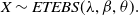 $X \sim ETEBS( \lambda,\beta, \theta).$
The ETEBS distribution exhibits a non-heavy right tail.
$X \sim ETEBS( \lambda,\beta, \theta).$
The ETEBS distribution exhibits a non-heavy right tail.
In Figure 1, the density and hazard rate functions of the sub-models within the ETE-G family are displayed. The densities exhibit various shapes, including symmetrical, right-skewed, and reverse-J forms, while the hazard rate functions may take on increasing, decreasing, bathtub, or upside-down bathtub patterns.
6. Application to Norwegian fire insurance claims data
In this section, sub-models of the ETE-G family of distributions are applied to analyze the complete Norwegian fire insurance claims data for the years 1972 through 1992, as studied by Beirlant et al. (Reference Beirlant, Teugels and Vynckier1996). The data consist of 9181 fire insurance losses in thousand Norwegian krone, ranging from 500 to 465,365 thousand Norwegian krone. In our modeling framework, we set the threshold parameter
 $\theta = d =500$
, aligning it with the deductible level. This reflects the structure of the ETE-G family, where
$\theta = d =500$
, aligning it with the deductible level. This reflects the structure of the ETE-G family, where
 $\theta$
defines the lower bound of the sub-models. For both data exploration and modeling, we focus on the 9020 claims exceeding 500 Norwegian kroner. The preliminary analysis shows a minimum of 500, maximum of 465,365, mean of 2248, first and third quartiles of 711 and 1817, respectively, and a skewness coefficient of 30.61. The skewness measure indicates that the data are highly positively skewed, and the quantile values show a large number of small losses and a small number of extreme losses. This exploratory analysis suggests that only highly skewed and heavy-tailed models can capture most of the characteristics of the given data. Other researchers have analyzed this dataset using different distributions and methodologies. (see Beirlant et al., Reference Beirlant, Matthys and Dierckx2001; Nadarajah and Bakar, Reference Nadarajah and Bakar2015; Mdziniso and Cooray, Reference Mdziniso and Cooray2018 and Brazauskas and Kleefeld, Reference Brazauskas and Kleefeld2016). However, our analysis does not compare sub-models of the ETE-G family of distributions to those studies, as we conduct our analysis without transforming the data or incorporating likelihood truncation.
$\theta$
defines the lower bound of the sub-models. For both data exploration and modeling, we focus on the 9020 claims exceeding 500 Norwegian kroner. The preliminary analysis shows a minimum of 500, maximum of 465,365, mean of 2248, first and third quartiles of 711 and 1817, respectively, and a skewness coefficient of 30.61. The skewness measure indicates that the data are highly positively skewed, and the quantile values show a large number of small losses and a small number of extreme losses. This exploratory analysis suggests that only highly skewed and heavy-tailed models can capture most of the characteristics of the given data. Other researchers have analyzed this dataset using different distributions and methodologies. (see Beirlant et al., Reference Beirlant, Matthys and Dierckx2001; Nadarajah and Bakar, Reference Nadarajah and Bakar2015; Mdziniso and Cooray, Reference Mdziniso and Cooray2018 and Brazauskas and Kleefeld, Reference Brazauskas and Kleefeld2016). However, our analysis does not compare sub-models of the ETE-G family of distributions to those studies, as we conduct our analysis without transforming the data or incorporating likelihood truncation.
We evaluated goodness-of-fit using both likelihood-based and distribution function-based criteria. The likelihood-based measures include Negative Log-Likelihood, Akaike Information Criterion (AIC), and Bayesian Information Criterion (BIC), while the distribution-based measures include the Kolmogorov–Smirnov (K-S), Anderson–Darling (A-D), and Cramér–von Mises (C-M) statistics, along with their simulated p-values.
The p-values for the K-S, A-D, and C-M test statistics are computed by simulating the test statistic values. This simulation is possible due to the closed-form quantile functions of the sub-models of the ETE-G family of distributions discussed in this article. Generally, a lower value of these goodness-of-fit statistics and a higher measure of p-values for the K-S, A-D and C-M indicate a better-fitting model.
To assess model performance, sub-models of the ETE-G family are compared with other Pareto-type distributions: the standard Pareto (Arnold, Reference Arnold2008), 3-parameter GPD (Coles et al., Reference Coles, Bawa, Trenner and Dorazio2001), exponentiated Pareto (Gupta et al., Reference Gupta, Gupta and Gupta1998), odd Pareto (Mdziniso and Cooray, Reference Mdziniso and Cooray2018), and beta-Pareto (Akinsete et al., Reference Akinsete, Famoye and Lee2008). For each model, parameter estimates, goodness-of-fit statistics, and corresponding p-values are computed and presented in Table 3, with standard errors and p-values in parentheses.
Table 3. Norwegian fire insurance claims 1972–1992. Estimated values for fitted distributions.
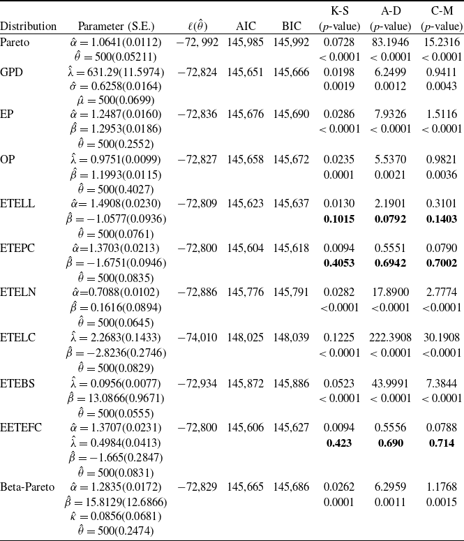
Note: Bold values are the best values.
From Table 3, it is evident that most ETE-G sub-models yield the lowest goodness-of-fit statistics, indicating superior performance compared to competing models considered in this article. In particular, the ETEPC distribution achieves the lowest negative log-likelihood, AIC, BIC, K-S, A-D, and C-M, along with higher p-values exceeding 5%, making it the preferred fitting model. It is remarkable to see this high p-value for the goodness-of-fit measures for such a large dataset. The EETEFC and ETELL distributions follow closely in overall performance. To further assess their adequacy, we examine the tail behavior of the three best-fitting models–ETEPC, EETEFC, and ETELL – using graphical diagnostics presented in Figure 2, where the top panels display Q–Q plots and the bottom panels show log–log survival plots.
The Q–Q plots reveal that the ETELL distribution provides a better visual fit to the extreme upper tail of the Norwegian claim data compared to the ETEPC distribution, despite ETEPC’s overall performance in terms of AIC, BIC, K-S, A-D, and C-M (see Tables 3 and 4). The log–log survival plots reinforce this result, clearly illustrating the fit of these models in the tail region. ETELL provides a noticeably better fit of the empirical survival function more closely than ETEPC and EETEFC, serving as a good explanatory model for the highest losses. This discrepancy highlights the limitation of relying solely on statistical goodness-of-fit measures, particularly the Anderson–Darling test, which, although designed to check the tail area fit, may lack power when the number of extreme values is relatively small. The Conditional Tail Expectation (CTE) values in Table 4 further support the use of ETELL in modeling large, extreme claims highlighting the need in actuarial applications to complement global fit measures with graphical diagnostics and tail-based metrics such as CTE.
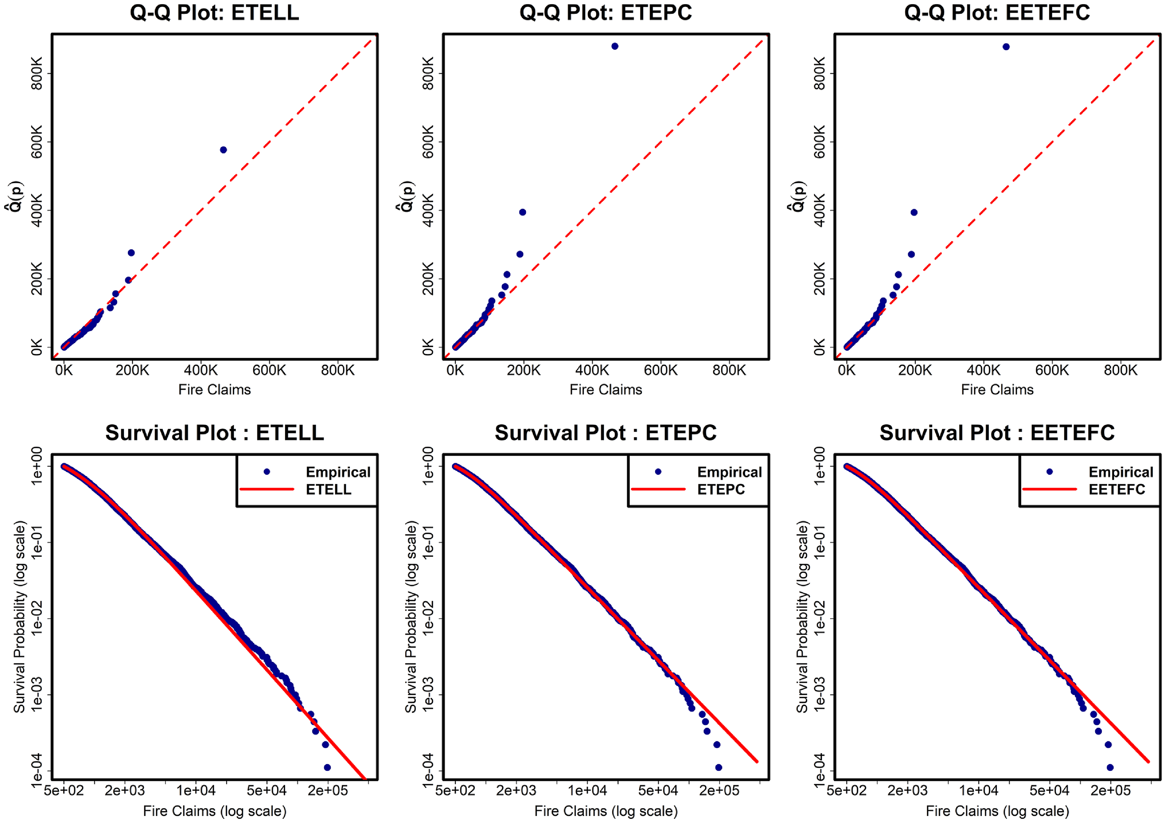
Figure 2. Q-Q plots for Norwegian fire insurance claims data (1972–1992) and log–log survival analysis. From left to right: ETELL, Enriched Truncated Exponentiated Power Cauchy (ETEPC), Enriched Extended Truncated Exponentiated Folded Cauchy (EETEFC).
Table 4. VaR and CTE values at different upper tail area and their backtesting results for the data.

6.1. Risk measures
In this subsection, we discuss two well-known risk measures, value at risk (VaR) and conditional tail expectation (CTE) to assess the adequacy of the fitted tails of the distributions to empirical measures.
Suppose X is a random variable that represents an insurance claim amount. Then the value at risk (VaR) is the 100pth percentile (also referred to as a quantile measure) of the distribution of X. For a given empirical cumulative distribution function
 $\hat{F}(.)$
of a continuous distribution, the empirical estimates of VaR, at
$\hat{F}(.)$
of a continuous distribution, the empirical estimates of VaR, at
 $1-\alpha_0$
level of confidence for upper tail, are defined as
$1-\alpha_0$
level of confidence for upper tail, are defined as
 \begin{align*} \text{VaR}_X(1-\alpha_0) = \hat{F}^{-1}(1-\alpha_0).\end{align*}
The theoretical estimates of VaR for the upper tail is given by
 \begin{align*}\text{VaR}_X(1-\alpha_0) = Q_0(1-\alpha_0).\end{align*}
where
 $Q_0(.)$
is the quantile function of the theoretical distribution.
$Q_0(.)$
is the quantile function of the theoretical distribution.
Conditional tail expectation (CTE), also known as the expected shortfall (ES) or tail value-at-risk (TVaR) is the expected value of X given that the random variable exceeds the VaR
 $(1-\alpha_0)$
threshold for the upper tail. The CTE has become increasingly popular due to its simplicity as well as its coherence. For a given empirical cumulative distribution function
$(1-\alpha_0)$
threshold for the upper tail. The CTE has become increasingly popular due to its simplicity as well as its coherence. For a given empirical cumulative distribution function
 $\hat{F}(.)$
of a continuous distribution, the empirical estimates of CTE at
$\hat{F}(.)$
of a continuous distribution, the empirical estimates of CTE at
 $1-\alpha_0$
level of confidence for the upper tail are defined as
$1-\alpha_0$
level of confidence for the upper tail are defined as
 \begin{align*} \text{CTE}_X(1-\alpha_0) = \dfrac{1}{1-\alpha_0}\int_{\alpha_0}^1\hat{F}^{-1}(s)ds = \dfrac{1}{1-\alpha_0}\int_{\alpha_0}^1\text{VaR}_X(1-\alpha_0)ds,\end{align*}
while the theoretical estimates of CTE of a continuous probability distribution with quantile
 $Q_0(x)$
are given by
$Q_0(x)$
are given by
 \begin{align*} \text{CTE}_X(1-\alpha_0) = \dfrac{1}{1-\alpha_0}\int_{\alpha_0}^1Q_0(s)ds.\end{align*}
Table 4 reports both empirical and theoretical estimates of VaR and CTE at various upper tail areas. The parameter estimates from Table 3 were used to compute the theoretical estimates for each risk measure.
6.2. Backtesting
We investigate the validity of these risk measures using the empirical backtesting approach by Bakar et al. (Reference Bakar, Hamzah, Maghsoudi and Nadarajah2015). The backtesting procedure examines whether the proportion of violations and the empirical mean of violations obtained using the theoretical estimates of VaR and CTE are consistent with the expected nominal levels of the two risk measures. This can be verified through a two-tailed binomial test comparing the proportion of violation observed to the nominal probability of VaR and through a two-tailed t-test comparing the CTE of each distribution with the average of the values that empirically exceed the VaR calculated using each distribution.
The empirical and theoretical estimate of VaR and CTE at 2%, 1%, and 0.5% upper tail areas for the Norwegian fire insurance data for ETELL, ETEPC, and EETEFC distributions are given in Table 4. These estimates provide a comprehensive understanding of tail risk across various levels of severity. Empirical backtesting could not be performed for other Pareto-type distributions and certain special models within the ETE-G family, as their estimated VaR values exceeded the maximum claim in the Norwegian insurance dataset or did not fit the data well.
The results show that the empirical VaR at 2%, 1%, and 0.5% upper tail areas matches well with the theoretical estimates of VaR for the Norwegian fire insurance claim data. At the 2% and 1% upper tail areas, the smallest difference, approximately 0.5%, is observed for the ETEPC and EETEFC distributions. Similarly, at the 0.5% upper tail area, the smallest difference of about 2.5% is also seen for the ETEPC and EETEFC distributions, indicating a strong match between empirical and theoretical VaR across different upper tail areas for these distributions.
The corresponding backtesting results for VaR at various upper tail areas are provided in Table 4. Based on the p-values obtained from the two-tailed binomial test, the ETELL, ETEPC, and EETEFC show acceptance of the null hypothesis across the various upper tail areas considered. This shows that the VaR estimates produced by these models are reasonable and appropriate for the Norwegian fire insurance claim data.
The empirical CTE does not match up very well with the theoretical CTE estimates at the 2%, 1%, and 0.5% upper tail area for the Norwegian fire insurance claim data. However, the smallest differences, around 3%, are observed for the ETELL distribution at the 2% and 1% upper tail areas, with a larger difference of approximately 10% at the 0.5% upper tail area. The corresponding backtesting results are provided in Table 4. Based on the p-values obtained from the t-test, the ETELL distribution shows acceptance of the null hypothesis, indicating that the ETELL distribution provides an appropriate fit for the right tail of the Norwegian insurance data across the different upper tail areas considered.
Underestimation poses a significant risk for this type of dataset. Therefore, a slight overestimation of empirical VaR and CTE is preferable, as it provides a more robust measure of risk than underestimation. It is reassuring that almost all theoretical estimates of CTE exceed empirical estimates, except for the theoretical CTE at the 2% upper tail area for the ETELL distribution, as these higher estimates provide sufficient allocation in calculating many quantities related to insurance. The larger differences between theoretical and empirical estimates may be attributed to the highly skewed tails of the Norwegian fire insurance dataset.
7. Conclusion
In this paper, we introduce the Enriched Truncated Exponentiated-G (ETE-G) family, a new family of distributions obtained by enriching truncated exponentiated baseline models to model loss payment data. Various properties of these new distributions are examined. Among the sub-models of this family, the ETELL is considered and its properties are studied. All sub-models within ETE-G family were fitted to the Norwegian fire insurance claims from 1972 to 1992. The results were compared to other Pareto-type distributions using several goodness-of-fit statistics.
The findings indicate that the sub-models of the ETE-G family consistently provide a better fit than competing models. Unlike other distributions in the literature, the sub-models of the ETE-G family offer a good fit without requiring any transformations on the data or incorporating likelihood truncation. These examples illustrate the usefulness of the ETE-G family for modeling heavy-tailed data.
Furthermore, two well-known risk measures, value at risk (VaR) and conditional tail expectation (CTE), which assess the adequacy of tail fitting, were calculated for the Norwegian fire insurance claims data. Empirical-based backtesting of the VaR and CTE test statistics was conducted to evaluate the performance of these tail risk measures.
Due to the flexibility introduced by the additional parameter in the model, the proposed ETE-G family of distributions is expected to attract broader applications in fields such as engineering, reliability analysis, survival and lifetime data, hydrology, economics, and beyond. Its ability to model various distributional shapes, as demonstrated by real-world dataset, highlights its potential to address diverse challenges. For future work, we plan to develop a more generalized framework that accommodates a broader range of distributions beyond those outlined as the baseline distributions in this study. This extension will also deepen the theoretical understanding and significantly broaden the applicability of these models to diverse insurance loss datasets, thereby promoting their practical relevance.
Supplementary material
The supplementary material for this article can be found at https://doi.org/10.1017/asb.2025.10081
Acknowledgments
The authors are grateful for the valuable suggestions of the editor, the associate editor, and the referees. Their insightful and constructive comments have substantially improved this article.
Appendices
Appendix A. Proof of Shannon Entropy
We derive the Shannon entropy
 $ H(X) = \mathbb{E}[{-}\ln f(x)] $
for the ETELL distribution
$ H(X) = \mathbb{E}[{-}\ln f(x)] $
for the ETELL distribution
 \begin{align*}H(X) &= -\int_\theta^\infty \ln f(x) \cdot f(x) \, dx \\[3pt] \nonumber&= -\ln\left( \frac{\alpha \beta \theta^\alpha}{2^\beta - 1} \right)+ (\alpha + 1) \int_\theta^\infty \ln x \cdot f(x) \, dx- (\beta - 1) \int_\theta^\infty \ln\left[1 + \left(\frac{\theta}{x}\right)^\alpha \right] f(x) \, dx\end{align*}
Using the substitution
 $ t = (\theta/x)^\alpha $
, the integrals simplify as
$ t = (\theta/x)^\alpha $
, the integrals simplify as
 \begin{align*}\int_\theta^\infty \ln x \cdot f(x) \, dx&= \ln \theta - \frac{\beta I_{\mathcal{B}-1}}{\alpha(2^\beta - 1)}, \\ \int_\theta^\infty \ln\left[1 + \left(\frac{\theta}{x}\right)^\alpha \right] f(x) \, dx&= \frac{\beta \cdot 2^\beta \ln 2 - 2^\beta + 1}{\beta (2^\beta - 1)},\end{align*}
where
 $ I_{\mathcal{B}-1} = \int_0^1 \ln t \cdot (1 + t)^{\beta - 1} dt $
. Substituting these results yields the closed-form entropy:
$ I_{\mathcal{B}-1} = \int_0^1 \ln t \cdot (1 + t)^{\beta - 1} dt $
. Substituting these results yields the closed-form entropy:
 \begin{align*}H(X) = -\ln\left[ \frac{\alpha \beta}{\theta(2^\beta - 1)} \right]- \frac{(\alpha + 1)\beta I_{\mathcal{B}-1}}{\alpha(2^\beta - 1)}- \frac{(\beta - 1)(\beta \cdot 2^\beta \ln 2 - 2^\beta + 1)}{\beta (2^\beta - 1)}.\end{align*}
Appendix B. Tail Index
Proof. Tail index for ETELL distribution using Equation (3.1)
 \begin{align*} \lim\limits_{t\to \infty} \dfrac{\overline{F}(tx)}{\overline{F} (t)} = \lim\limits_{t\to \infty} \dfrac{\left[1+\left( \frac{\theta}{tx}\right)^\alpha\right]^\beta-1}{\left[1+\left( \frac{\theta}{t}\right)^\alpha\right]^\beta-1} = \lim\limits_{t\to \infty} \dfrac{\beta \left(\dfrac{\theta}{x}\right)^\alpha + \dfrac{\beta(\beta-1)}{2!}\left(\dfrac{\theta^{2\alpha}}{t^\alpha x^{2\alpha}}\right) + \cdots }{\beta \left(\dfrac{\theta}{1}\right)^\alpha + \dfrac{\beta(\beta-1)}{2!}\left(\dfrac{\theta^{2\alpha}}{t^\alpha}\right) + \cdots } =x^{-1/(\frac{1}{\alpha})}\end{align*}
Proof. Tail index for ETEPC distribution using Equation (3.1)
 \begin{align*} \lim\limits_{t\to \infty} \dfrac{\overline{F}(tx)}{\overline{F} (t)} = \lim\limits_{t\to \infty} \dfrac{\dfrac{-2\beta}{\pi}\frac{\alpha}{1+\left( \frac{tx}{\theta}\right)^{2\alpha} }\left( \dfrac{tx}{\theta}\right)^{\alpha-1}\left(\dfrac{x}{\theta}\right)\left[\dfrac{2}{\pi}\tan^{-1}\left(\dfrac{tx}{\theta}\right)^\alpha\right]^{-\beta-1}}{\dfrac{-2\beta}{\pi}\frac{\alpha}{1+\left( \frac{t}{\theta}\right)^{2\alpha} }\left( \dfrac{t}{\theta}\right)^{\alpha-1}\left(\dfrac{1}{\theta}\right)\left[\dfrac{2}{\pi}\tan^{-1}\left(\dfrac{t}{\theta}\right)^\alpha\right]^{-\beta-1}} &=x^{-1/(\frac{1}{\alpha})}\end{align*}
Proof. Tail index for EETEFC distribution using Equation (3.1)
 \begin{align*} \lim\limits_{t\to \infty} \dfrac{\overline{F}(tx)}{\overline{F} (t)} &=\lim\limits_{t\to \infty} \dfrac{\left[ \left( \dfrac{x}{\theta}\right)^\alpha + \left( \dfrac{\theta}{t^2x}\right)^\alpha\right]\left[ t^{-2\alpha}+\lambda^2\left[ \left( \frac{1}{\theta}\right)^\alpha - \left(\frac{\theta}{t^2}\right)^\alpha\right]^2\right]}{\left[ \left( \dfrac{1}{\theta}\right)^\alpha + \left( \dfrac{\theta}{t^2}\right)^\alpha\right]\left[ t^{-2\alpha}+\lambda^2\left[ \left( \frac{x}{\theta}\right)^\alpha - \left(\frac{\theta}{t^2x}\right)^\alpha\right]^2\right]} =x^{-1/(\frac{1}{\alpha})}\end{align*}
Appendix C. Relative Tail Heaviness
Using the ratio of the pdf between
 $ETELL(\alpha,\beta,\theta)$
and
$ETELL(\alpha,\beta,\theta)$
and
 $OP(\alpha_0,\beta_0,\theta_0)$
distribution in (3.2)
$OP(\alpha_0,\beta_0,\theta_0)$
distribution in (3.2)
 \begin{align*}\lim\limits_{x \rightarrow \infty} \frac{f_{ETELL}(\mathbf{x,\alpha,\beta,\theta})}{f_{OP}(\mathbf{x,\alpha_0,\beta_0,\theta_0})}& = K\lim\limits_{x \rightarrow \infty} \frac{ {x^{-(\alpha+1)}} \left[ 1+\left(\frac{\theta}{x}\right)^\alpha\right]^{\beta-1} }{x^{\alpha_0-1}\left(\frac{x}{\theta_0}\right)^{-\alpha_0\beta_0-\alpha_0}\left[ 1 - \left(\dfrac{\theta_0}{x} \right)\right]^{\beta_0-1} \left\{\left(\dfrac{\theta_0}{x} \right)^{\alpha_0\beta_0}+\left[1-\left(\frac{\theta_0}{x} \right)^{\alpha_0}\right]^{\beta_0}\right\}^{-2}}\\&= K\lim\limits_{x \rightarrow \infty}x^{(\alpha_0\beta_0-\alpha)}\end{align*}
Appendix D. Uniqueness of Maximum Likelihood Estimators
Derivative with respect to
 $\mathbf{\beta}$
:
$\mathbf{\beta}$
:
 \begin{align*}g^{\prime}(\beta) &= -\frac{n}{\beta^2} + \frac{2^\beta \cdot n \ln^2(2)}{(2^\beta - 1)^2} \\&= -\frac{n}{\beta^2(2^\beta - 1)^2} \left[(2^\beta - 1)^2 - 2^\beta \beta^2 \ln^2(2)\right] \\&= -\frac{n}{\beta^2(2^\beta - 1)^2} \left[1 + 2^{2\beta} - 2 \cdot 2^\beta - 2^\beta \beta^2 \ln^2(2) \right] \\&= -\frac{n}{\beta^2(2^\beta - 1)^2} \left[1 + 2^\beta \left(2^\beta - 2 - \beta^2 \ln^2(2) \right) \right]\end{align*}
Using the series expansion
 $ 2^\beta = e^{\beta \ln 2} = 1 + \beta \ln 2 + \frac{\beta^2 \ln^2(2)}{2!} + \frac{\beta^3 \ln^3(2)}{3!} + \cdots $
, we find:
$ 2^\beta = e^{\beta \ln 2} = 1 + \beta \ln 2 + \frac{\beta^2 \ln^2(2)}{2!} + \frac{\beta^3 \ln^3(2)}{3!} + \cdots $
, we find:
 \begin{align*}g^{\prime}(\beta)&= -\frac{n}{\beta^2(2^\beta - 1)^2} \left[\left(1 + \beta \ln 2 + \frac{\beta^2 \ln^2(2)}{2} + \cdots \right)\left(-1 + \beta \ln 2 - \frac{\beta^2 \ln^2(2)}{2} + \cdots \right) + 1\right] \\[2pt] \nonumber&= -\frac{n}{\beta^2(2^\beta - 1)^2} \left[\frac{\beta^4 \ln^4(2)}{8} + \mathcal{O}(\beta^5)\right]\end{align*}
This proves the existence and uniqueness of the ml estimator for
 $\beta$
whenever
$\beta$
whenever
 $\lvert \beta \rvert \le 1.$
Derivative with respect to
 $\mathbf{\alpha}$
:
$\mathbf{\alpha}$
:
 \begin{align*}g^{\prime}(\alpha)&= \sum_{i=1}^n \left[\frac{1 + \beta \left( \frac{\theta}{x_i} \right)^\alpha}{1 + \left( \frac{\theta}{x_i} \right)^\alpha}\right] \ln \left( \frac{\theta}{x_i} \right) \\[2pt] \nonumber&\quad + \alpha \beta \sum_{i=1}^n \left[\frac{\left( \frac{\theta}{x_i} \right)^\alpha}{1 + \left( \frac{\theta}{x_i} \right)^\alpha}\right] \ln^2 \left( \frac{\theta}{x_i} \right)- \alpha \sum_{i=1}^n \left[\frac{\left(1 + \beta \left( \frac{\theta}{x_i} \right)^\alpha\right) \left( \frac{\theta}{x_i} \right)^\alpha}{\left[ 1 + \left( \frac{\theta}{x_i} \right)^\alpha \right]^2}\right] \ln^2 \left( \frac{\theta}{x_i} \right) \\&= \sum_{i=1}^n \left[\frac{1 + \beta \left( \frac{\theta}{x_i} \right)^\alpha}{1 + \left( \frac{\theta}{x_i} \right)^\alpha}\right] \ln \left( \frac{\theta}{x_i} \right)+ \alpha (\beta - 1) \sum_{i=1}^n \left\{\frac{\left( \frac{\theta}{x_i} \right)^\alpha}{\left[1 + \left( \frac{\theta}{x_i} \right)^\alpha \right]^2}\right\} \ln^2 \left( \frac{\theta}{x_i} \right)\end{align*}
This proves the existence and uniqueness of the ml estimator for
 $\alpha$
when
$\alpha$
when
 $\lvert \beta \rvert \le 1$
.
$\lvert \beta \rvert \le 1$
.

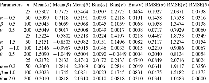
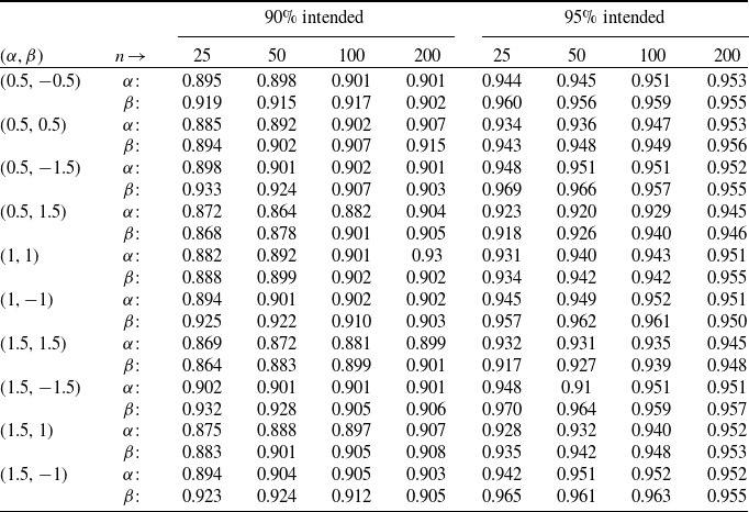

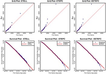
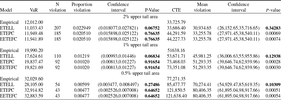


 Open access