


1. Introduction
Liquid droplets formed through the emulsification of immiscible liquids are ubiquitous in nature and widely used in industrial, biological and pharmaceutical applications. Their controlled transport under applied electric fields has enabled advancements in droplet-based microfluidics (Shui, Eijkel & Van den Berg Reference Shui, Eijkel and Van den Berg2007; Teh et al. Reference Teh, Lin, Hung and Lee2008), lab-on-a-chip devices (Haeberle & Zengerle Reference Haeberle and Zengerle2007), biomedical microelectromechanical system applications (Katsura et al. Reference Katsura, Yamaguchi, Inami, Matsuura, Hirano and Mizuno2001), targeted drug delivery, separation of biomolecules (e.g. RNA, DNA, proteins) (Keren Reference Keren2003), food toxin analysis (Juan-García et al. Reference Juan-García, Font and Picó2005) and oil recovery technologies (Qi et al. Reference Qi, Sun, Li, Chen, Liu and Li2022). Droplet manipulation minimises cross-contamination and enhances mixing efficiency, making it essential in processes ranging from cosmetics to food processing (Okochi & Nakano Reference Okochi and Nakano2000; Dickinson Reference Dickinson2011). Additionally, droplets serve as models for biological entities like cells and vesicles (Hochmuth et al. Reference Hochmuth, Ting-Beall, Beaty, Needham and Tran-Son-Tay1993; Lim, Zhou & Quek Reference Lim, Zhou and Quek2006), and their motion and deformation in viscous media play a critical role in crude-oil industries and colloid science (Frising, Noïk & Dalmazzone Reference Frising, Noïk and Dalmazzone2006; Abeynaike et al. Reference Abeynaike, Sederman, Khan, Johns, Davidson and Mackley2012).
The electrophoresis of liquid droplets fundamentally differs from that of rigid particles due to the occurrence of Maxwell traction at the interface coupled with hydrodynamic stresses, and interfacial tension effects (Baygents & Saville Reference Baygents and Saville1991). Based on the Debye–Hückel approximation, Booth (Reference Booth1951) provided an analytical expression for the electrophoretic mobility of dielectric droplets by considering a uniformly charged and non-deformable interface with no surface tension gradients. Ohshima, Healy & White (Reference Ohshima, Healy and White1984) extended this framework to consider the electrophoresis of conducting mercury droplets with uniform surface charge density, providing mobility expressions under the assumptions of low
 $\zeta$
-potential as well as beyond the Debye–Hückel regime with thin-layer consideration, while ignoring surface tension effects. Recent studies (e.g. Schnitzer, Frankel & Yariv Reference Schnitzer, Frankel and Yariv2014; Wu et al. Reference Wu, Fan, Jian and Lee2021) on the electrophoresis of non-polarisable droplets with uniform surface charge have found a discontinuous variation of mobility with surface charge density or
$\zeta$
-potential as well as beyond the Debye–Hückel regime with thin-layer consideration, while ignoring surface tension effects. Recent studies (e.g. Schnitzer, Frankel & Yariv Reference Schnitzer, Frankel and Yariv2014; Wu et al. Reference Wu, Fan, Jian and Lee2021) on the electrophoresis of non-polarisable droplets with uniform surface charge have found a discontinuous variation of mobility with surface charge density or
 $\zeta$
-potential. Mahapatra, Ohshima & Gopmandal (Reference Mahapatra, Ohshima and Gopmandal2022) analysed the electrophoresis of polarisable hydrophobic droplets of constant surface charge density with no Marangoni effects and derived analytical expressions for the mobility within the Debye–Hückel regime. While these models provide valuable insights under idealised conditions, they do not capture the coupling between surface charge transport, interfacial flow and surface tension gradients that arises in the presence of adsorbed ionic surfactants. The presence of surfactant molecules that adsorb at the interface further modifies the droplet dynamics (Levich Reference Levich1962; Manikantan & Squires Reference Manikantan and Squires2020). Surfactants, which stabilise the droplet interface, can redistribute due to advection, diffusion and interfacial electric stresses. This redistribution creates gradients in interfacial tension, resulting in Marangoni stresses. These stresses significantly alter the electrophoretic mobility of droplets, often resulting in behaviour distinct from that of rigid particles or surfactant-free droplets. Understanding these dynamics is vital for optimising drug delivery, oil recovery and advanced materials.
$\zeta$
-potential. Mahapatra, Ohshima & Gopmandal (Reference Mahapatra, Ohshima and Gopmandal2022) analysed the electrophoresis of polarisable hydrophobic droplets of constant surface charge density with no Marangoni effects and derived analytical expressions for the mobility within the Debye–Hückel regime. While these models provide valuable insights under idealised conditions, they do not capture the coupling between surface charge transport, interfacial flow and surface tension gradients that arises in the presence of adsorbed ionic surfactants. The presence of surfactant molecules that adsorb at the interface further modifies the droplet dynamics (Levich Reference Levich1962; Manikantan & Squires Reference Manikantan and Squires2020). Surfactants, which stabilise the droplet interface, can redistribute due to advection, diffusion and interfacial electric stresses. This redistribution creates gradients in interfacial tension, resulting in Marangoni stresses. These stresses significantly alter the electrophoretic mobility of droplets, often resulting in behaviour distinct from that of rigid particles or surfactant-free droplets. Understanding these dynamics is vital for optimising drug delivery, oil recovery and advanced materials.
The modelling of ionic surfactants at fluid–fluid interfaces remains an area of active research, with no clear consensus on how to accurately describe the charge distribution at the interface. Kralchevsky et al. (Reference Kralchevsky, Danov, Broze and Mehreteab1999) and Kralchevsky & Danov (Reference Kralchevsky and Danov2015) describe a thermodynamically consistent model for surface tension isotherms at interfaces with adsorbed ionic or non-ionic species which are in equilibrium with the adjacent diffuse electric double layer (EDL). Depending on the granularity of the modelling approach for the interface and its surface tension isotherm, this allows a consistent coarse-grained treatment of an effective interface comprising both surface layer and EDL as a lumped model or a detailed microscopic approach with a separate treatment of the surface isotherm for the adsorbed species and a resolved diffuse ion cloud. The contribution related to surface adsorption can be modelled by one of the commonly employed surface isotherms such as the Langmuir, Vollmer or Frumkin isotherms (Kralchevsky et al. Reference Kralchevsky, Danov, Broze and Mehreteab1999; Kralchevsky & Danov Reference Kralchevsky and Danov2015; Manikantan & Squires Reference Manikantan and Squires2020), while a Gouy–Chapman model can be applied to describe the EDL. This approach also facilitates a thermodynamically consistent treatment of specifically adsorbed counterions forming a ’Stern layer’ on the surfactant layer. A similar modelling approach was already adopted by Baygents & Saville (Reference Baygents and Saville1991) for analysing the electrophoresis of drops and bubbles, albeit using a simple Henry isotherm for the surface model and a resolved ion cloud modelled by the Poisson–Nernst–Planck equations appropriate under dilute conditions. Prosser & Franses (Reference Prosser and Franses2001) and Ivanov, Ananthapadmanabhan & Lips (Reference Ivanov, Ananthapadmanabhan and Lips2006) review coarse-grained equilibrium surface tension models for the description of experimentally obtained surface tension isotherms.
Hill & Afuwape (Reference Hill and Afuwape2020) developed a thin-double-layer approximation retaining temporal fluid inertia to investigate the mobility of nano-drops in the presence of charged surfactants with no exchange of surfactant between the interface and the immediately adjacent electrolyte under oscillating applied electric and sonic pressure fields. Subsequently, Hill (Reference Hill2020) presented an exact numerical solution for the electrophoresis of surfactant-stabilised emulsion drops including the surfactant exchange kinetics. Experimental interpretations of these theoretical studies (Hill & Afuwape Reference Hill and Afuwape2020; Hill Reference Hill2020) are made in Afuwape & Hill (Reference Afuwape and Hill2021) by measuring the dynamic mobility spectra as well as interfacial tension isotherms of oil drops with irreversibly adsorbed charged surfactants and also illustrated the effects due to Marangoni and Maxwell stresses. These studies address discrepancies between measured mobilities and inferred
 $\zeta$
-potentials, suggesting that the use of the Smoluchowski formula may not fully capture the complexities of surfactant effects at highly charged interfaces even for thin double layers. Building on this foundation, Hill (Reference Hill2025) investigated the impact of both irreversibly bound and soluble surfactants on droplet electrophoresis through numerical simulation based on the first-order perturbation from equilibrium. In that study it is demonstrated that the singularity in the electrophoretic mobility of a droplet, which occurs as its uniform, immobile surface charge density is varied, is regularised when the surface charge is considered mobile. Based on the Debye–Hückel approximation, Ohshima (Reference Ohshima2025a
) derived an analytical expression for the electrophoretic mobility of an oil drop that acquires its surface charge through ion adsorption following a linear adsorption isotherm, assuming instantaneous interfacial equilibrium between adsorbed and dissolved surfactants. The linear isotherm neglects finite site saturation effects, which can strongly influence interfacial Marangoni stresses at high surfactant coverage. He further showed that the resulting expression is independent of the drop’s relative dielectric permittivity. That work was subsequently extended to gel media (Ohshima Reference Ohshima2025b
). However, existing studies on the electrophoresis of droplets have not derived analytical solutions beyond the Debye–Hückel approximation for droplets laden with ionic surfactants.
$\zeta$
-potentials, suggesting that the use of the Smoluchowski formula may not fully capture the complexities of surfactant effects at highly charged interfaces even for thin double layers. Building on this foundation, Hill (Reference Hill2025) investigated the impact of both irreversibly bound and soluble surfactants on droplet electrophoresis through numerical simulation based on the first-order perturbation from equilibrium. In that study it is demonstrated that the singularity in the electrophoretic mobility of a droplet, which occurs as its uniform, immobile surface charge density is varied, is regularised when the surface charge is considered mobile. Based on the Debye–Hückel approximation, Ohshima (Reference Ohshima2025a
) derived an analytical expression for the electrophoretic mobility of an oil drop that acquires its surface charge through ion adsorption following a linear adsorption isotherm, assuming instantaneous interfacial equilibrium between adsorbed and dissolved surfactants. The linear isotherm neglects finite site saturation effects, which can strongly influence interfacial Marangoni stresses at high surfactant coverage. He further showed that the resulting expression is independent of the drop’s relative dielectric permittivity. That work was subsequently extended to gel media (Ohshima Reference Ohshima2025b
). However, existing studies on the electrophoresis of droplets have not derived analytical solutions beyond the Debye–Hückel approximation for droplets laden with ionic surfactants.
Experimentally, it is widespread practice to interpret the electrophoretic mobility of drops or bubbles assuming a fully immobilised interface (e.g. Hunter Reference Hunter1981; Yang et al. Reference Yang, Dabros, Li, Czarnecki and Masliyah2001; Pullanchery et al. Reference Pullanchery, Kulik, Okur, De Aguiar and Roke2020), often rationalised by the effect of adsorbed surfactant on the compressibility of the interface. Wuzhang et al. (Reference Wuzhang, Song, Sun, Pan and Li2015) measured the electrophoretic mobility of droplets in the presence of charged surfactants but did not attempt to model their results. Instead, they invoked the formation of a stagnant cap on certain regions of the interface to explain the vortices observed in their experiments.
Most of the existing theories on electrophoresis are based on simplified assumptions, such as ion as point charge (O’Brien & White Reference O’Brien and White1978; Ohshima et al. Reference Ohshima, Healy and White1983, Reference Ohshima, Healy and White1984; Kim, Nakayama & Yamamoto Reference Kim, Nakayama and Yamamoto2006), which neglects hydrodynamic steric hindrance between ions (Khair & Squires Reference Khair and Squires2009) and ion–ion correlations (Bazant, Storey & Kornyshev Reference Bazant, Storey and Kornyshev2011). The electrokinetics for such cases is governed by the standard electrokinetic model (SEM), based on the Poisson–Nernst–Planck–Navier–Stokes equations (O’Brien & White Reference O’Brien and White1978; Kim et al. Reference Kim, Nakayama and Yamamoto2006; Schnitzer et al. Reference Schnitzer, Frankel and Yariv2013, Reference Schnitzer, Frankel and Yariv2014; Cobos & Khair Reference Cobos and Khair2023). These assumptions suffice for dilute electrolytes and low surface charge densities but fail to capture the non-ideal behaviour at a high ionic concentration of electrolytes or highly charged interfaces. In such cases, the finite size of ions introduces steric interactions that limit the accumulation of counterions near the surface, creating counterion saturation. Ion–ion electrostatic correlations become significant in multivalent electrolytes (Storey & Bazant Reference Storey and Bazant2012; Stout & Khair Reference Stout and Khair2014; de Souza & Bazant Reference de Souza and Bazant2020), modifying the structure of the EDL (Gupta et al. Reference Gupta, Govind Rajan, Carter and Stone2020). Consideration of the ion–ion correlations in electrokinetics can explain several non-ideal phenomena such as like-charge attraction, occurrence of reversal in mobility of a charged particle in multivalent counterions and the development of a layered structure of ions in the EDL (Semenov et al. Reference Semenov, Raafatnia, Sega, Lobaskin, Holm and Kremer2013; Kubíčková et al. Reference Kubíčková, Křížek, Coufal, Vazdar, Wernersson, Heyda and Jungwirth2012; Agrawal, Duan & Wang Reference Agrawal, Duan and Wang2023).
Under a continuum hypothesis, Bazant et al. (Reference Bazant, Storey and Kornyshev2011) and Storey & Bazant (Reference Storey and Bazant2012) developed a model which accounts for the correlations of finite-sized ions based on the non-local electrostatic approach (Hildebrandt et al. Reference Hildebrandt, Blossey, Rjasanow, Kohlbacher and Lenhof2004). This model is implemented by several authors (Stout & Khair Reference Stout and Khair2014; Alidoosti & Zhao Reference Alidoosti and Zhao2018; Misra et al. Reference Misra, de Souza, Blankschtein and Bazant2019; Paik, Bhattacharyya & Majhi Reference Paik, Bhattacharyya and Majhi2024) to illustrate the electrokinetics of rigid colloids in multivalent electrolytes and demonstrate the layering structure of ions in EDL and electrophoretic mobility reversal. This model also provides better agreement of the mobility of colloids with experimental observations (Stout & Khair Reference Stout and Khair2014; Paik et al. Reference Paik, Bhattacharyya and Majhi2024). However, similar investigations on liquid droplets are yet to be conducted. Recently, Majhi & Bhattacharyya (Reference Majhi and Bhattacharyya2024) examined droplet electrophoresis by incorporating ion steric interactions under the assumption of neutral surfactants on charged surfaces, demonstrating rigidification in the presence of neutral surfactants. However, they did not account for the electrostatic ion–ion correlation effects in their model, which manifests for multivalent electrolytes. In the recent past, several experimental studies (Li & Somasundaran Reference Li and Somasundaran1991, Reference Li and Somasundaran1992) have reported mobility reversal of gaseous bubbles in multivalent electrolytes, which cannot be explained based on the mean-field-based electrokinetic models. Nevertheless, no theoretical attempt to elucidate such phenomena in the context of fluid droplets has been made. Thus, a unified treatment that combines surfactant dynamics with short-range correlations and steric interactions of finite-sized ions is important in the context of droplet electrophoresis.
In this paper, a mathematical model is developed to describe the electrophoresis of droplets laden with insoluble, compressible ionic surfactants, which are irreversibly bound to the interface and do not exchange with the surrounding electrolyte medium during the flow. A modified electrokinetic formulation, MEMC (modified electrokinetic model with correlations), is employed, which incorporates ion steric interactions and electrostatic ion–ion correlations of finite-sized ions. The hydrodynamic ion steric interaction is governed by the Boublík–Mansoori–Carnahan–Starling–Leland (BMCSL) equation of state (Boublík Reference Boublík1970; Bazant et al. Reference Bazant, Kilic, Storey and Ajdari2009). As the ions are considered as finite-sized, the viscosity of the electrolyte medium and, consequently, the diffusivity of ions vary with the local ionic volume fraction, which are modelled by the Batchelor–Green two-particle hydrodynamics framework (Batchelor & Green Reference Batchelor and Green1972). Electrostatic ion–ion correlations are integrated into the model based on the Bazant–Storey–Kornyshev approach (Bazant et al. Reference Bazant, Storey and Kornyshev2011), which modifies the classical Poisson equation into the fourth-order modified Poisson equation for the electric potential.
Our analysis is based on the numerical solution of the resulting equations describing the electrokinetics up to linear order in the applied electric field. It is worth noting that the numerical solution of the full set of electrokinetic equations does not deviate from the present approach for a moderate range of the applied electric field. The present MEMC reduces to the point-charge-based SEM for certain values of the parameters. We derive analytical solutions based on the SEM under the Debye–Hückel approximation, valid for a range of surface charge density for which the surface potential is lower than the thermal potential, as well as under the thin-Debye-layer consideration applicable for an arbitrary equilibrium surface potential. Under certain conditions the present Debye–Hückel-based solution reduces to several existing analytical expressions for mobility. Through the numerical solution of our modified model, we have shown the mobility reversal in droplet electrophoresis in a trivalent electrolyte. This study advances the theoretical understanding of droplet electrophoresis incorporating non-ideal effects in ion transport to get further insights into droplet electrophoresis, which may offer guidance for the design and optimisation of droplet-based nanofluidics and emulsion-based technologies.
2. Mathematical model
We consider the electrophoresis of a surfactant-laden liquid spherical droplet of radius
 $a$
immersed in an incompressible ionised fluid of permittivity
$a$
immersed in an incompressible ionised fluid of permittivity
 $\epsilon _e$
and viscosity
$\epsilon _e$
and viscosity
 $\mu ^{*}_{e}$
moving with electrophoretic velocity
$\mu ^{*}_{e}$
moving with electrophoretic velocity
 $U^{^*}_{E}$
in response to an external electric field
$U^{^*}_{E}$
in response to an external electric field
 $\boldsymbol{E}^{\infty }$
. The fluid inside the droplet is incompressible, immiscible with the outer fluid and electrically neutral and its viscosity is
$\boldsymbol{E}^{\infty }$
. The fluid inside the droplet is incompressible, immiscible with the outer fluid and electrically neutral and its viscosity is
 $\overline {\mu }$
. There is no electrolyte ionic species inside the droplet or no electrolyte ion can penetrate through its surface. The surface charge
$\overline {\mu }$
. There is no electrolyte ionic species inside the droplet or no electrolyte ion can penetrate through its surface. The surface charge
 $\sigma ^{*}$
is created due to the presence of insoluble charged surfactant molecules at the droplet surface and it can be obtained as
$\sigma ^{*}$
is created due to the presence of insoluble charged surfactant molecules at the droplet surface and it can be obtained as
 $\sigma ^{*}=\sum _{i}{z_{s,i}e\varGamma ^{*}_{i}}$
, where
$\sigma ^{*}=\sum _{i}{z_{s,i}e\varGamma ^{*}_{i}}$
, where
 $\varGamma ^{*}_{i}$
and
$\varGamma ^{*}_{i}$
and
 $z_{s,i}$
are the concentration and valency of
$z_{s,i}$
are the concentration and valency of
 $i\text{th}$
components of the surfactant. Variables with an asterisk are dimensional. A spherical polar coordinate system (
$i\text{th}$
components of the surfactant. Variables with an asterisk are dimensional. A spherical polar coordinate system (
 $r,\theta ,\psi$
) is adopted with its origin fixed at the centre of the droplet and the
$r,\theta ,\psi$
) is adopted with its origin fixed at the centre of the droplet and the
 $z$
axis (
$z$
axis (
 $\theta = 0$
) along the imposed electric field
$\theta = 0$
) along the imposed electric field
 $\boldsymbol{E}^{\infty }$
. Figure 1 provides a schematic illustration of the problem under consideration.
$\boldsymbol{E}^{\infty }$
. Figure 1 provides a schematic illustration of the problem under consideration.

Figure 1. Schematic diagram of a surfactant-laden spherical droplet moving with electrophoretic velocity
 $U^{*}_{E}$
under the impact of external electric field
$U^{*}_{E}$
under the impact of external electric field
 $\boldsymbol{E}^{\infty }=E^{\infty }\boldsymbol{e_z}$
in an electrolyte solution where hydrated radius and valency of cations (subscript ‘+’) and anions (subscript ‘−’) are given by
$\boldsymbol{E}^{\infty }=E^{\infty }\boldsymbol{e_z}$
in an electrolyte solution where hydrated radius and valency of cations (subscript ‘+’) and anions (subscript ‘−’) are given by
 $R_{+,-}$
and
$R_{+,-}$
and
 $z_{+,-}$
, respectively.
$z_{+,-}$
, respectively.
For a highly charged surface in an electrolyte with multivalent counterions the electric coupling parameter providing the ratio between the inter-ionic spacing and the Guoy–Chapman length becomes large. In this case the mobile ions are laterally correlated with the surface charge (Grosberg, Nguyen & Shklovskii Reference Grosberg, Nguyen and Shklovskii2002). In order to account for the impact of electrostatic ion–ion correlations, Bazant et al. (Reference Bazant, Storey and Kornyshev2011) developed a fourth-order modified Poisson equation (MPE) for electric potential based on the non-local electrostatic approach. This introduces an additional parameter, the correlation length
 $\ell _{c}$
, which is bounded by the ion diameter (lower limit) and
$\ell _{c}$
, which is bounded by the ion diameter (lower limit) and
 $V^{2}_{c}l_{B}$
(upper limit). Here,
$V^{2}_{c}l_{B}$
(upper limit). Here,
 $V_{c}$
is the valency of the counterion and
$V_{c}$
is the valency of the counterion and
 $\ell _{B}=e^2/4\pi \epsilon _e k_BT$
is the Bjerrum length. The latter corresponds to the distance at which the electrostatic interaction energy between a pair of monovalent ions equals the thermal energy; in aqueous medium,
$\ell _{B}=e^2/4\pi \epsilon _e k_BT$
is the Bjerrum length. The latter corresponds to the distance at which the electrostatic interaction energy between a pair of monovalent ions equals the thermal energy; in aqueous medium,
 $\ell _{B}\sim 0.7\,\textrm{nm}$
. If the distance between ions exceeds
$\ell _{B}\sim 0.7\,\textrm{nm}$
. If the distance between ions exceeds
 $\ell _{c}$
, they primarily experience mean-field electrostatics. However, when the distance is smaller than
$\ell _{c}$
, they primarily experience mean-field electrostatics. However, when the distance is smaller than
 $\ell _{c}$
, Coulombic electrostatic correlations become significant, requiring a higher-order correction to the traditional Poisson equation. The MPE is written as
$\ell _{c}$
, Coulombic electrostatic correlations become significant, requiring a higher-order correction to the traditional Poisson equation. The MPE is written as
 \begin{equation} \epsilon _e\left({{\nabla} ^{*}}^{2}\psi ^{*}-\ell ^{2}_{c}{{\nabla} ^{*}}^{4}\psi ^{*}\right)=-\rho ^{*}_e, \end{equation}
where
 $\psi ^{*}$
is the electrostatic potential and
$\psi ^{*}$
is the electrostatic potential and
 $\rho ^{*}_e=\sum _{i=1}^{N}{z_{i}en^{*}_{i}}$
is the space charge density in which
$\rho ^{*}_e=\sum _{i=1}^{N}{z_{i}en^{*}_{i}}$
is the space charge density in which
 $n^{*}_{i}$
is the ionic concentration of the
$n^{*}_{i}$
is the ionic concentration of the
 $i{\text{th}}$
ionic species with valency
$i{\text{th}}$
ionic species with valency
 $z_{i}$
. Upon non-dimensionalising, using the droplet radius
$z_{i}$
. Upon non-dimensionalising, using the droplet radius
 $a$
as length scale, (2.1) becomes
$a$
as length scale, (2.1) becomes
 \begin{equation} {\nabla}^{2}\psi -\frac {\delta ^{2}_{c}}{(\kappa a)^{2}}{\nabla}^{4}\psi =-\frac {(\kappa a)^{2}}{2}\sum _{i=1}^{N}{z_{i}n_{i}}, \end{equation}
where
 $\psi$
and
$\psi$
and
 $n_{i}$
are, respectively, the dimensionless electric potential, scaled by the thermal potential,
$n_{i}$
are, respectively, the dimensionless electric potential, scaled by the thermal potential,
 $\psi _{0}=k_{B}T/e$
, and the ionic concentration of the
$\psi _{0}=k_{B}T/e$
, and the ionic concentration of the
 $i{\text{th}}$
ionic species, scaled by the bulk ionic strength,
$i{\text{th}}$
ionic species, scaled by the bulk ionic strength,
 $I$
. Length
$I$
. Length
 $\kappa ^{-1}$
is the Debye length defined as
$\kappa ^{-1}$
is the Debye length defined as
 $\kappa ^{-1}=\sqrt {\epsilon _e\psi _{0}/2Ie}$
and
$\kappa ^{-1}=\sqrt {\epsilon _e\psi _{0}/2Ie}$
and
 $I$
is the ionic strength in the bulk defined by
$I$
is the ionic strength in the bulk defined by
 $I=(1/2)\sum _{i=1}^{N}{z^{2}_{i}n^{\infty }_{i}}$
, where
$I=(1/2)\sum _{i=1}^{N}{z^{2}_{i}n^{\infty }_{i}}$
, where
 $n^{\infty }_{i}$
is the dimensional bulk concentration of the
$n^{\infty }_{i}$
is the dimensional bulk concentration of the
 $i\text{th}$
ionic species. Length
$i\text{th}$
ionic species. Length
 $\delta _{c}$
is the dimensionless correlation length scaled by
$\delta _{c}$
is the dimensionless correlation length scaled by
 $\kappa ^{-1}$
, i.e.
$\kappa ^{-1}$
, i.e.
 $\delta _{c}=\ell _{c}\kappa$
. De Souza & Bazant (Reference de Souza and Bazant2020) provide a power-law relationship of
$\delta _{c}=\ell _{c}\kappa$
. De Souza & Bazant (Reference de Souza and Bazant2020) provide a power-law relationship of
 $\delta _{c}$
in terms of the Gouy–Chapman length,
$\delta _{c}$
in terms of the Gouy–Chapman length,
 $\ell _{GC}$
, the Bjerrum length,
$\ell _{GC}$
, the Bjerrum length,
 $V^{2}_{c}\ell _{B}$
, and the Debye length,
$V^{2}_{c}\ell _{B}$
, and the Debye length,
 $\kappa ^{-1}$
, and can be expressed as
$\kappa ^{-1}$
, and can be expressed as
 \begin{equation} \delta _{c}=0.35\left (\frac {V^{2}_{c}\ell _{B}}{\ell _{GC}}\right )^{- 1/8}\left (\frac {V^{2}_{c}\ell _{B}}{\kappa ^{-1}}\right )^{ 2/3}, \end{equation}
where
 $\ell _{GC}$
can be calculated as
$\ell _{GC}$
can be calculated as
 $\ell _{GC}=e(2\pi V_{c}\ell _{B}\sigma ^{*})^{-1}$
in which
$\ell _{GC}=e(2\pi V_{c}\ell _{B}\sigma ^{*})^{-1}$
in which
 $\sigma ^{*}$
is the surface charge density at the droplet surface. In order to solve the MPE for electric potential, the following boundary condition can be imposed at the droplet interface:
$\sigma ^{*}$
is the surface charge density at the droplet surface. In order to solve the MPE for electric potential, the following boundary condition can be imposed at the droplet interface:
 \begin{equation} \boldsymbol{n}\boldsymbol{\cdot }\left ({\nabla} ^{*}\psi ^{*}-\ell ^{2}_{c}{{\nabla} ^{*}}^{3}\psi ^{*}\right )=-\frac {\sigma ^{*}}{\epsilon _e}. \end{equation}
Here,
 $\boldsymbol{n}$
is the outward unit normal vector at the surface. We assume that the electric permittivity
$\boldsymbol{n}$
is the outward unit normal vector at the surface. We assume that the electric permittivity
 $\epsilon _d$
of the droplet is much smaller than the permittivity of the surrounding fluid,
$\epsilon _d$
of the droplet is much smaller than the permittivity of the surrounding fluid,
 $\epsilon _d \ll \epsilon _e$
, as is usually suitable for oil droplets in water. In this case, the electric field variation inside the droplet has a negligible influence on boundary conditions such as (2.4) at the interface (Schnitzer et al. Reference Schnitzer, Frankel and Yariv2014; Wu et al. Reference Wu, Fan, Jian and Lee2021).
$\epsilon _d \ll \epsilon _e$
, as is usually suitable for oil droplets in water. In this case, the electric field variation inside the droplet has a negligible influence on boundary conditions such as (2.4) at the interface (Schnitzer et al. Reference Schnitzer, Frankel and Yariv2014; Wu et al. Reference Wu, Fan, Jian and Lee2021).
In the present study, we restrict ourselves to a single adsorbed species with surface concentration
 $\varGamma ^{*}$
and valency
$\varGamma ^{*}$
and valency
 $z_{s}$
. In this case,
$z_{s}$
. In this case,
 $\sigma ^{*}=z_{s}e\varGamma ^{*}$
. The dimensionless form of the above boundary condition (2.4) is obtained as
$\sigma ^{*}=z_{s}e\varGamma ^{*}$
. The dimensionless form of the above boundary condition (2.4) is obtained as
 \begin{equation} \boldsymbol{n}\boldsymbol{\cdot }\left (\boldsymbol{\nabla }\psi -\frac {\delta ^{2}_{c}}{(\kappa a)^{2}}{\nabla} ^{3}\psi \right )=-\sigma . \end{equation}
The dimensionless surface charge density
 $\sigma$
is given by
$\sigma$
is given by
 $\sigma =z_{s}Ma\varGamma$
, in which the surfactant concentration
$\sigma =z_{s}Ma\varGamma$
, in which the surfactant concentration
 $\varGamma ^{*}$
is scaled by
$\varGamma ^{*}$
is scaled by
 $\varGamma ^{\infty }$
. Here
$\varGamma ^{\infty }$
. Here
 $\varGamma ^{\infty }$
is the maximum packing surface concentration of the surfactant at the interface and
$\varGamma ^{\infty }$
is the maximum packing surface concentration of the surfactant at the interface and
 $\textit{Ma}$
is the Marangoni number defined as
$\textit{Ma}$
is the Marangoni number defined as
 $\textit{Ma}=ea\varGamma ^{\infty }/\epsilon _e\psi _{0}$
, or equivalently,
$\textit{Ma}=ea\varGamma ^{\infty }/\epsilon _e\psi _{0}$
, or equivalently,
 $\textit{Ma}=k_{B}T\varGamma ^{\infty }/\mu U_{0}$
. In the present formulation,
$\textit{Ma}=k_{B}T\varGamma ^{\infty }/\mu U_{0}$
. In the present formulation,
 $\textit{Ma}$
represents the ratio of the characteristic surfactant-induced surface-pressure stress,
$\textit{Ma}$
represents the ratio of the characteristic surfactant-induced surface-pressure stress,
 $k_B T\,\varGamma ^\infty /a$
, to the characteristic viscous stress,
$k_B T\,\varGamma ^\infty /a$
, to the characteristic viscous stress,
 $\mu U_0/a$
. Here,
$\mu U_0/a$
. Here,
 $U_0=\epsilon _e \psi _0^{2}/a\mu$
is the velocity scale and
$U_0=\epsilon _e \psi _0^{2}/a\mu$
is the velocity scale and
 $\mu$
is the dynamic viscosity of the electrolyte at infinite dilution. The dielectric displacement vector with non-local electrostatic consideration becomes
$\mu$
is the dynamic viscosity of the electrolyte at infinite dilution. The dielectric displacement vector with non-local electrostatic consideration becomes
 $\boldsymbol{D}^{*}=\epsilon _e(\ell ^{2}_{c}{{\nabla} ^{*}}^{2}-1)\boldsymbol{E^{*}}$
, and with that the Maxwell stress
$\boldsymbol{D}^{*}=\epsilon _e(\ell ^{2}_{c}{{\nabla} ^{*}}^{2}-1)\boldsymbol{E^{*}}$
, and with that the Maxwell stress
 $S^{*}_{E}$
becomes (de Souza & Bazant Reference de Souza and Bazant2020)
$S^{*}_{E}$
becomes (de Souza & Bazant Reference de Souza and Bazant2020)
 \begin{align} S^{*}_{E}&=\epsilon _e\left [\boldsymbol{E^{*}E^{*}}-\frac {1}{2}{E^{*}}^2 \boldsymbol{I}\right ]\nonumber\\ &\quad +\epsilon _e\ell ^{2}_{c}\left [(\boldsymbol{E^{*}}\boldsymbol{\cdot }{{\nabla} ^{*}}^{2}\boldsymbol{E^{*}})\boldsymbol{I}-\boldsymbol{E^{*}}({{\nabla} ^{*}}^{2}\boldsymbol{E^{*}})-({{\nabla} ^{*}}^{2}\boldsymbol{E^{*}})\boldsymbol{E^{*}}+\frac {1}{2}({{\nabla} ^{*}}\boldsymbol{\cdot }\boldsymbol{E^{*}})^{2}\boldsymbol{I}\right ]\!. \end{align}
Here
 $\boldsymbol{E}^{*}=-{\nabla} ^{*} \psi ^{*}$
,
$\boldsymbol{E}^{*}=-{\nabla} ^{*} \psi ^{*}$
,
 $(E^{*})^2=\boldsymbol{E^{*}\boldsymbol{\cdot }E^{*}}$
and
$(E^{*})^2=\boldsymbol{E^{*}\boldsymbol{\cdot }E^{*}}$
and
 $\boldsymbol{E^{*}E^{*}}$
denotes the dyadic product. The first term represents the classical tangential electrostatic stress exerted by the field on the interfacial surface charge, while the second term arises from ion–ion correlation effects. Using (2.4), the tangential electric stress at the interface is obtained as
$\boldsymbol{E^{*}E^{*}}$
denotes the dyadic product. The first term represents the classical tangential electrostatic stress exerted by the field on the interfacial surface charge, while the second term arises from ion–ion correlation effects. Using (2.4), the tangential electric stress at the interface is obtained as
 \begin{equation} \boldsymbol{n}\boldsymbol{\cdot }S^{*}_{E}\boldsymbol{\cdot }\boldsymbol{t}=-z_{s}e\varGamma ^{*}\frac {1}{a}\frac {\partial \psi ^{*}}{\partial \theta }+\epsilon _e \ell ^{2}_{c}\frac {\partial \psi ^*}{\partial r}{\nabla} ^{3}\psi ^*\boldsymbol{\cdot }\boldsymbol{t}. \end{equation}
As the droplet is considered non-polarisable, i.e.
 $\epsilon _d \ll \epsilon _e$
, the permittivity contrast between the droplet and the electrolyte medium is negligibly small so that the internal Maxwell stress tensor,
$\epsilon _d \ll \epsilon _e$
, the permittivity contrast between the droplet and the electrolyte medium is negligibly small so that the internal Maxwell stress tensor,
 $\overline {S}^{*}_{\overline {E}} = \epsilon _d [ \boldsymbol{\overline {E}^{*}\,\overline {E}^{*}} - ({1}/{2}){\overline {E}^{*}}^2 \boldsymbol{I}]$
, where
$\overline {S}^{*}_{\overline {E}} = \epsilon _d [ \boldsymbol{\overline {E}^{*}\,\overline {E}^{*}} - ({1}/{2}){\overline {E}^{*}}^2 \boldsymbol{I}]$
, where
 $\overline {\boldsymbol{E}}^{*}$
is the internal electric field of the droplet, becomes much smaller than the external contribution and is therefore neglected in the interfacial stress balance condition. The electric force on the surface charge is governed by tangential electric field at the interface, i.e.
$\overline {\boldsymbol{E}}^{*}$
is the internal electric field of the droplet, becomes much smaller than the external contribution and is therefore neglected in the interfacial stress balance condition. The electric force on the surface charge is governed by tangential electric field at the interface, i.e.
 $-({1}/{a})({\partial \psi ^{*}}/{\partial \theta })$
, and the corresponding tangential force density is
$-({1}/{a})({\partial \psi ^{*}}/{\partial \theta })$
, and the corresponding tangential force density is
 $-\sigma ^{*}({1}/{a})({\partial \psi ^{*}}/{\partial \theta })$
, which is
$-\sigma ^{*}({1}/{a})({\partial \psi ^{*}}/{\partial \theta })$
, which is
 $-z_{s}e\varGamma ^{*}({1}/{a})({\partial \psi ^{*}}/{\partial \theta })$
(
$-z_{s}e\varGamma ^{*}({1}/{a})({\partial \psi ^{*}}/{\partial \theta })$
(
 $-z_{s}Ma\varGamma ({\partial \psi }/{\partial \theta })$
in scaled form). This implies that the second term on the right-hand side of (2.7) has to vanish at the interface, which provides the additional boundary condition at the interface to solve the MPE, i.e.
$-z_{s}Ma\varGamma ({\partial \psi }/{\partial \theta })$
in scaled form). This implies that the second term on the right-hand side of (2.7) has to vanish at the interface, which provides the additional boundary condition at the interface to solve the MPE, i.e.
 \begin{equation} \boldsymbol{t}\boldsymbol{\cdot }{{\nabla} ^{*}}^{3}\psi ^{*}=0 \end{equation}
and in dimensionless form
 \begin{equation} \boldsymbol{t}\boldsymbol{\cdot }{{\nabla} }^{3}\psi =0. \end{equation}
Further, with (2.8) we have at the interface
 \begin{equation} \boldsymbol{n}\boldsymbol{\cdot }S^{*}_{E}\boldsymbol{\cdot }\boldsymbol{t}=-z_{s}e\varGamma ^{*}\frac {1}{a}\frac {\partial \psi ^{*}}{\partial \theta }. \end{equation}
The equations of motion for the ionised incompressible Newtonian electrolyte outside the droplet can be expressed in non-dimensional form as
 \begin{align}\boldsymbol{\nabla }p +\mu _e \boldsymbol{\nabla }\times \boldsymbol{\nabla }\times \boldsymbol{u}-\boldsymbol{\nabla }\mu _{e}\boldsymbol{\cdot }[\boldsymbol{\nabla }\boldsymbol{u}+(\boldsymbol{\nabla }\boldsymbol{u})^T]+ \frac {(\kappa a)^{2}}{2} \rho _e \boldsymbol{\nabla }\psi =0,\end{align}
 \begin{align}\boldsymbol{\nabla }\boldsymbol{\cdot }\boldsymbol{u}=0 ,\end{align}
where
 $\boldsymbol{u}=v \boldsymbol{e}_r + u \boldsymbol{e}_\theta$
is the velocity vector,
$\boldsymbol{u}=v \boldsymbol{e}_r + u \boldsymbol{e}_\theta$
is the velocity vector,
 $v$
is the radial velocity component,
$v$
is the radial velocity component,
 $u$
is the cross-radial velocity component and
$u$
is the cross-radial velocity component and
 $p$
is the pressure. The above equations are obtained by scaling the dimensional variables as follows: the length scale is the radius of the sphere
$p$
is the pressure. The above equations are obtained by scaling the dimensional variables as follows: the length scale is the radius of the sphere
 $a$
,
$a$
,
 $U_0=\epsilon _e \psi _0^{2}/a\mu$
is the velocity scale, as previously mentioned,
$U_0=\epsilon _e \psi _0^{2}/a\mu$
is the velocity scale, as previously mentioned,
 $\tau =a/U_0$
is the time scale and
$\tau =a/U_0$
is the time scale and
 $\epsilon _e \psi _0^{2}/a^{2}$
is the pressure scale. If we consider the ions as finite-sized charged spheres suspended in the medium, then the viscosity of the medium must vary with the local volume fraction of ions. The variation of viscosity of the electrolyte medium with ionic volume fraction
$\epsilon _e \psi _0^{2}/a^{2}$
is the pressure scale. If we consider the ions as finite-sized charged spheres suspended in the medium, then the viscosity of the medium must vary with the local volume fraction of ions. The variation of viscosity of the electrolyte medium with ionic volume fraction
 $\varPhi$
is governed by the Batchelor–Green expression (Batchelor & Green Reference Batchelor and Green1972):
$\varPhi$
is governed by the Batchelor–Green expression (Batchelor & Green Reference Batchelor and Green1972):
 \begin{equation} \mu _{e}=1+2.5\varPhi +5.2\varPhi ^{2}, \end{equation}
in which
 $\mu _{e}$
is the viscosity of the electrolyte medium, scaled by
$\mu _{e}$
is the viscosity of the electrolyte medium, scaled by
 $\mu$
and
$\mu$
and
 $\varPhi$
is the local ionic volume fraction defined as
$\varPhi$
is the local ionic volume fraction defined as
 $\varPhi =\sum _{i}{Iv_{i}n_{i}}$
, where
$\varPhi =\sum _{i}{Iv_{i}n_{i}}$
, where
 $v_i=(4/3)\pi R^{3}_{i}$
is the volume of the
$v_i=(4/3)\pi R^{3}_{i}$
is the volume of the
 $i{\text{th}}$
ionic species with hydrated radius
$i{\text{th}}$
ionic species with hydrated radius
 $R_{i}$
. The non-dimensional equation for the flow inside the droplet is
$R_{i}$
. The non-dimensional equation for the flow inside the droplet is
 \begin{align} \mu _{r} {\nabla}^{2}\overline {\boldsymbol{u}}-\boldsymbol{\nabla }\overline {p}&=0, \end{align}
 \begin{align} \boldsymbol{\nabla }\boldsymbol{\cdot }\overline {\boldsymbol{u}}&=0 , \end{align}
where
 $\overline {\boldsymbol{u}}=\overline {v} \boldsymbol{e}_r +\overline { u} \boldsymbol{e}_\theta$
is the velocity vector and
$\overline {\boldsymbol{u}}=\overline {v} \boldsymbol{e}_r +\overline { u} \boldsymbol{e}_\theta$
is the velocity vector and
 $\overline {p}$
is the pressure inside the droplet. Ratio
$\overline {p}$
is the pressure inside the droplet. Ratio
 $\mu _{r}\ (=\overline {\mu }/\mu )$
is the viscosity ratio between the viscosity inside the drop and the viscosity of the outside electrolyte at infinite dilution. We assume that the droplet region is free of electrolytes, i.e. it contains no free ions, which implies
$\mu _{r}\ (=\overline {\mu }/\mu )$
is the viscosity ratio between the viscosity inside the drop and the viscosity of the outside electrolyte at infinite dilution. We assume that the droplet region is free of electrolytes, i.e. it contains no free ions, which implies
 $\overline {\rho }_e = 0$
. Therefore, there is no electrical body force term in (2.14). The conservation law for the
$\overline {\rho }_e = 0$
. Therefore, there is no electrical body force term in (2.14). The conservation law for the
 $i\text{th}$
ionic species is
$i\text{th}$
ionic species is
 \begin{equation} \boldsymbol{\nabla }\boldsymbol{\cdot }\boldsymbol{N}_{i}=0, \end{equation}
where
 $\boldsymbol{N}_{i}$
is the molar flux of the
$\boldsymbol{N}_{i}$
is the molar flux of the
 $i{\text{th}}$
ionic species defined as
$i{\text{th}}$
ionic species defined as
 \begin{equation} \boldsymbol{N}_{i}=n_{i}\boldsymbol{u}-\frac {1}{{\textit{Pe}}_{i}}D_{i}n_{i}\boldsymbol{\nabla }\mu _{i}, \end{equation}
in which
 $\mu _{i}$
is the dimensionless electrochemical potential given by
$\mu _{i}$
is the dimensionless electrochemical potential given by
 \begin{equation} \mu _{i}=\mu _{i0}+z_{i}\psi +\ln {n_{i}}+\mu ^{\textit{ex}}_{i}. \end{equation}
The term
 $\mu ^{\textit{ex}}_{i}$
, known as the excess electrochemical potential, accounts for short-range steric repulsion due to the finite size of ions, and its effect is characterised by the bulk ionic volume fraction,
$\mu ^{\textit{ex}}_{i}$
, known as the excess electrochemical potential, accounts for short-range steric repulsion due to the finite size of ions, and its effect is characterised by the bulk ionic volume fraction,
 $\varPhi (\infty )=\sum _{i}{v_{i}n^{\infty }_{i}}$
. When
$\varPhi (\infty )=\sum _{i}{v_{i}n^{\infty }_{i}}$
. When
 $\varPhi (\infty ) \sim \mathcal{O}(0.1)$
, the steric interactions significantly influence the ionic concentration distribution, thereby modifying the local charge density. This, in turn, alters the electric potential, which affects the electrostatic forces governing fluid motion, ultimately leading to changes in the velocity field. Therefore, under such conditions, the contribution of
$\varPhi (\infty ) \sim \mathcal{O}(0.1)$
, the steric interactions significantly influence the ionic concentration distribution, thereby modifying the local charge density. This, in turn, alters the electric potential, which affects the electrostatic forces governing fluid motion, ultimately leading to changes in the velocity field. Therefore, under such conditions, the contribution of
 $\mu ^{\textit{ex}}_{i}$
cannot be neglected. Based on the BMCSL equation of state (Boublík Reference Boublík1970),
$\mu ^{\textit{ex}}_{i}$
cannot be neglected. Based on the BMCSL equation of state (Boublík Reference Boublík1970),
 $\mu ^{\textit{ex}}_{i}$
can be expressed as
$\mu ^{\textit{ex}}_{i}$
can be expressed as
 \begin{align} \mu ^{\textit{ex}}_{i} = &-\left [1+2\left (\frac {\alpha _{2}R_{i}}{\varPhi }\right )^{3}-3\left (\frac {\alpha _{2}R_{i}}{\varPhi }\right )^{2}\right ]\ln (1-\varPhi )+\frac {3\alpha _{2}R_{i}+3\alpha _{1}R^{2}_{i}+\alpha _{0}R^{3}_{i}}{1-\varPhi }\nonumber\\ & +\frac {3\alpha _{2}R^{2}_{i}}{(1-\varPhi )^{2}}\left (\frac {\alpha _{2}}{\varPhi }+\alpha _{1}R_{i}\right )-\alpha ^{3}_{2}R^{3}_{i}\frac {\varPhi ^{2}-5\varPhi +2}{\varPhi ^{2}(1-\varPhi )^{3}}. \end{align}
The quantity
 $\alpha _{k}$
is defined as
$\alpha _{k}$
is defined as
 $\alpha _{k}=\sum _{i}{Iv_{i}R^{k-3}_{i}n_{i}}$
. We consider the BMCSL model as it regards each ion to have a different radius, whereas the Carnahan–Starling equation of state assumes the hydrated radius of all ions as equal, taken as the average of the hydrated radii of cation and anion. The additional term
$\alpha _{k}=\sum _{i}{Iv_{i}R^{k-3}_{i}n_{i}}$
. We consider the BMCSL model as it regards each ion to have a different radius, whereas the Carnahan–Starling equation of state assumes the hydrated radius of all ions as equal, taken as the average of the hydrated radii of cation and anion. The additional term
 $\mu ^{\textit{ex}}_{i}$
in the electrochemical potential disappears when ions are treated as point charges, i.e. when
$\mu ^{\textit{ex}}_{i}$
in the electrochemical potential disappears when ions are treated as point charges, i.e. when
 $R_i=0$
. We refer to the present framework as the MEMC, which reduces to the SEM when
$R_i=0$
. We refer to the present framework as the MEMC, which reduces to the SEM when
 $\ell _{c}=0$
and
$\ell _{c}=0$
and
 $R_i=0$
. Since the viscosity of the electrolyte depends on the local ionic volume fraction, the diffusion coefficient of the
$R_i=0$
. Since the viscosity of the electrolyte depends on the local ionic volume fraction, the diffusion coefficient of the
 $i{\text{th}}$
ionic species,
$i{\text{th}}$
ionic species,
 $D_{i}$
, also varies with the local volume fraction, and is prescribed as
$D_{i}$
, also varies with the local volume fraction, and is prescribed as
 \begin{equation} D_{i}=(1+2.5\varPhi +5.2\varPhi ^{2})^{-1}. \end{equation}
In (2.17),
 ${\textit{Pe}}_i=\epsilon _e \psi _0^{2}/\mu D^{\infty }_i$
is the Péclet number of the
${\textit{Pe}}_i=\epsilon _e \psi _0^{2}/\mu D^{\infty }_i$
is the Péclet number of the
 $i{\text{th}}$
ionic species, characterising the ratio of advective to diffusion transport of ions in which
$i{\text{th}}$
ionic species, characterising the ratio of advective to diffusion transport of ions in which
 $D^{\infty }_i$
is the diffusion coefficient of the
$D^{\infty }_i$
is the diffusion coefficient of the
 $i{\text{th}}$
ion at infinite dilution. The boundary conditions for the velocity field and ion concentration at the droplet surface (
$i{\text{th}}$
ion at infinite dilution. The boundary conditions for the velocity field and ion concentration at the droplet surface (
 $r=1$
) are the continuity of tangential velocity, assuming no molecular slip, as well as fluid and ion impermeability conditions, i.e.
$r=1$
) are the continuity of tangential velocity, assuming no molecular slip, as well as fluid and ion impermeability conditions, i.e.
 \begin{equation} \boldsymbol{u}=\overline {\boldsymbol{u}},\,\,\,\,\,\boldsymbol{u}\boldsymbol{\cdot }\boldsymbol{n}=0,\,\,\,\,\,\boldsymbol{N}_{i}\boldsymbol{\cdot }\boldsymbol{n}=0. \end{equation}
The stress balance condition is crucial in droplet electrophoresis and is significantly influenced by the presence of ionic surfactants at the interface. The tangential stress balance condition is given as (Slattery, Sagis & Oh Reference Slattery, Sagis and Oh2007; Manikantan & Squires Reference Manikantan and Squires2020)
 \begin{equation} \boldsymbol{n}\boldsymbol{\cdot }(S^{*}_{H}-\overline {S}^{*}_{H})\boldsymbol{\cdot }\boldsymbol{t}=-{\nabla} ^{*}_{s}\gamma ^{*}\boldsymbol{\cdot }\boldsymbol{t}, \end{equation}
where
 $S^{*}_{H}$
is the hydrodynamic stress, i.e.
$S^{*}_{H}$
is the hydrodynamic stress, i.e.
 $S^{*}_{H}=-p^{*}\boldsymbol{I}+\mu ^{*}_{e}[{\nabla} ^{*} \boldsymbol{u}^{*} + ({\nabla} ^{*} \boldsymbol{u}^{*})^T]$
,
$S^{*}_{H}=-p^{*}\boldsymbol{I}+\mu ^{*}_{e}[{\nabla} ^{*} \boldsymbol{u}^{*} + ({\nabla} ^{*} \boldsymbol{u}^{*})^T]$
,
 $\gamma ^{*}$
represents the surface tension and
$\gamma ^{*}$
represents the surface tension and
 ${\nabla} ^{*}_{s}=(\boldsymbol{I}-\boldsymbol{n}\boldsymbol{n})\boldsymbol{\cdot }{\nabla} ^{*}$
is the gradient along the surface. Here, the surface gradient of
${\nabla} ^{*}_{s}=(\boldsymbol{I}-\boldsymbol{n}\boldsymbol{n})\boldsymbol{\cdot }{\nabla} ^{*}$
is the gradient along the surface. Here, the surface gradient of
 $\gamma ^*$
contains the tangential Maxwell stress as explained in the following. According to the Gibbs adsorption isotherm,
$\gamma ^*$
contains the tangential Maxwell stress as explained in the following. According to the Gibbs adsorption isotherm,
 \begin{equation} -{\nabla} ^{*}_{s}\gamma ^{*}={\nabla} ^{*}_{s}\varPi ^{*}=\sum _i \varGamma ^*_i{\nabla} ^{*}_{s}\mu ^*_{s,i}, \end{equation}
where
 $\varPi ^*$
is the surface pressure due to adsorption of components
$\varPi ^*$
is the surface pressure due to adsorption of components
 $i$
at the interface with interface concentrations
$i$
at the interface with interface concentrations
 $\varGamma ^{*}_{i}$
and
$\varGamma ^{*}_{i}$
and
 $\mu ^*_{s,i}$
is the electrochemical potential at the interface due to the surfactant concentration. Assuming a single surfactant species characterised by a Langmuir isotherm, the electrochemical potential of the surfactant is (Manikantan & Squires Reference Manikantan and Squires2020)
$\mu ^*_{s,i}$
is the electrochemical potential at the interface due to the surfactant concentration. Assuming a single surfactant species characterised by a Langmuir isotherm, the electrochemical potential of the surfactant is (Manikantan & Squires Reference Manikantan and Squires2020)
 \begin{equation} \mu ^{*}_{s}=\mu ^{*}_{s0}+k_{B}T\ln \frac {\varGamma ^{*}}{\varGamma ^{\infty }-\varGamma ^{*}}+z_{s}e\psi ^{*}_{s}. \end{equation}
Substituting in (2.23) and simplifying yields
 \begin{equation} -{\nabla} ^{*}_{s}\gamma ^{*}=k_{B}T\frac {\varGamma ^{*}}{\varGamma ^{\infty }-\varGamma ^{*}}{\nabla} ^{*}_{s}\varGamma ^{*}+z_{s}e\varGamma ^{*}{\nabla} ^{*}_{s}\psi ^{*}_{s}. \end{equation}
Substituting (2.25) into the tangential stress balance condition (2.22), we obtain
 \begin{equation} \boldsymbol{n}\boldsymbol{\cdot }(S^{*}_{H}-\overline {S}^{*}_{H})\boldsymbol{\cdot }\boldsymbol{t}=k_{B}T\frac {\varGamma ^{*}}{\varGamma ^{\infty }-\varGamma ^{*}}{\nabla} ^{*}_{s}\varGamma ^{*}\boldsymbol{\cdot }\boldsymbol{t}+z_{s}e\varGamma ^{*}{\nabla} ^{*}_{s}\psi ^{*}_{s}\boldsymbol{\cdot }\boldsymbol{t}. \end{equation}
The final term of the above equation can be expressed as
 $z_{s}e\varGamma ^{*}{\nabla} ^{*}_{s}\psi ^{*}_{s}\boldsymbol{\cdot }\boldsymbol{t}=-\boldsymbol{n}\boldsymbol{\cdot }S^{*}_{E}\boldsymbol{\cdot }\boldsymbol{t}$
from (2.10). The tangential stress balance condition, arising through the balance of electric, hydrodynamic and Marangoni stresses (Baygents & Saville Reference Baygents and Saville1991; Vlahovska Reference Vlahovska2019), can thus be recast as
$z_{s}e\varGamma ^{*}{\nabla} ^{*}_{s}\psi ^{*}_{s}\boldsymbol{\cdot }\boldsymbol{t}=-\boldsymbol{n}\boldsymbol{\cdot }S^{*}_{E}\boldsymbol{\cdot }\boldsymbol{t}$
from (2.10). The tangential stress balance condition, arising through the balance of electric, hydrodynamic and Marangoni stresses (Baygents & Saville Reference Baygents and Saville1991; Vlahovska Reference Vlahovska2019), can thus be recast as
 \begin{equation} \boldsymbol{n}\boldsymbol{\cdot }(S^{*}_{H}-\overline {S}^{*}_{H})\boldsymbol{\cdot }\boldsymbol{t}+\boldsymbol{n}\boldsymbol{\cdot }S^{*}_{E}\boldsymbol{\cdot }\boldsymbol{t}=k_{B}T\frac {\varGamma ^{*}}{\varGamma ^{\infty }-\varGamma ^{*}}{\nabla} ^{*}_{s}\varGamma ^{*}\boldsymbol{\cdot }\boldsymbol{t}. \end{equation}
It may be noted that the contribution to the Maxwell stress from the interior of the droplet can be neglected as
 $\epsilon _d \ll \epsilon _e$
. Upon applying the necessary substitutions, non-dimensionalising and performing algebraic simplifications, (2.27) reduces to
$\epsilon _d \ll \epsilon _e$
. Upon applying the necessary substitutions, non-dimensionalising and performing algebraic simplifications, (2.27) reduces to
 \begin{equation} \mu _{e}\left (\frac {\partial u}{\partial r}-\frac {u}{r}\right )\bigg |_{r=1^+}-\mu _r \left (\frac {\partial \overline {u}}{\partial r}-\frac {\overline {u}}{r}\right )\bigg |_{r=1^-} ={\left [z_{s}Ma\varGamma \frac {\partial \psi }{\partial \theta }\right ]}_{r=1}+\frac {Ma}{1-\varGamma }\frac {\partial \varGamma }{\partial \theta }. \end{equation}
The left-hand side of (2.28) represents the hydrodynamic stress jump across the interface and the first term on the right-hand side accounts for the tangential Maxwell stress. The last term in (2.28) arises due to the surface pressure of the surfactant present at the interface of the droplet.
Throughout this study, we assume that the droplet retains a spherical shape under the influence of an applied electric field
 $\boldsymbol{E}^{\infty }$
. This assumption is justified in the weak-field regime, characterised by the dimensionless parameter
$\boldsymbol{E}^{\infty }$
. This assumption is justified in the weak-field regime, characterised by the dimensionless parameter
 $ \varLambda = aeE^{\infty }/k_B T \ll 1$
. As shown in classical works by Taylor (Reference Taylor1964), Torza, Cox & Mason (Reference Torza, Cox and Mason1971) and Baygents & Saville (Reference Baygents and Saville1991), deformation of the droplet surface arises only at
$ \varLambda = aeE^{\infty }/k_B T \ll 1$
. As shown in classical works by Taylor (Reference Taylor1964), Torza, Cox & Mason (Reference Torza, Cox and Mason1971) and Baygents & Saville (Reference Baygents and Saville1991), deformation of the droplet surface arises only at
 $\mathcal{O}(\varLambda ^2)$
, which corresponds to the electric capillary number
$\mathcal{O}(\varLambda ^2)$
, which corresponds to the electric capillary number
 $Ca_E = \epsilon _e {E^{\infty }}^2 a/\gamma ^{*}$
(Vlahovska Reference Vlahovska2019). In the weak-field limit,
$Ca_E = \epsilon _e {E^{\infty }}^2 a/\gamma ^{*}$
(Vlahovska Reference Vlahovska2019). In the weak-field limit,
 $Ca_E \ll 1$
, indicating that electric stresses are negligible compared with surface tension, and the droplet shape remains spherical. Since our analysis is carried out up to
$Ca_E \ll 1$
, indicating that electric stresses are negligible compared with surface tension, and the droplet shape remains spherical. Since our analysis is carried out up to
 $\mathcal{O}(\varLambda )$
, shape deformations are beyond the leading-order accuracy and are thus neglected. To illustrate, consider a typical oil droplet of radius
$\mathcal{O}(\varLambda )$
, shape deformations are beyond the leading-order accuracy and are thus neglected. To illustrate, consider a typical oil droplet of radius
 $a = 100\,\textrm{nm}$
in water with interfacial tension
$a = 100\,\textrm{nm}$
in water with interfacial tension
 $\gamma ^{*} \approx 10^{-2}\,\text{N m}^{-1}$
, subject to an electric field
$\gamma ^{*} \approx 10^{-2}\,\text{N m}^{-1}$
, subject to an electric field
 $E^{\infty } = 10^4\,\text{V m}^{-1}$
, and with water permittivity
$E^{\infty } = 10^4\,\text{V m}^{-1}$
, and with water permittivity
 $\epsilon _e= 7.0832 \times 10^{-10}\,\text{F m}^{-1}$
. The electric capillary number evaluates to
$\epsilon _e= 7.0832 \times 10^{-10}\,\text{F m}^{-1}$
. The electric capillary number evaluates to
 $Ca_E=7.0832 \times 10^{-7} \ll 1$
, confirming that droplet deformation is negligible for realistic field strengths in our regime of interest.
$Ca_E=7.0832 \times 10^{-7} \ll 1$
, confirming that droplet deformation is negligible for realistic field strengths in our regime of interest.
Moreover, the variation of surface tension on the drop due to mobile surfactants influences the pressure jump across the interface. With the Young–Laplace equation an estimate for the relative change in the radius of curvature due to these surface tension variations is
 $\Delta a/a \sim \Delta \gamma ^{*} / \gamma ^{*} \sim kT\Delta \varGamma ^* / \gamma ^{*}$
for not too large surface coverage. In this study, we have considered
$\Delta a/a \sim \Delta \gamma ^{*} / \gamma ^{*} \sim kT\Delta \varGamma ^* / \gamma ^{*}$
for not too large surface coverage. In this study, we have considered
 $\varGamma ^{\infty }$
up to
$\varGamma ^{\infty }$
up to
 $2\,\textrm{nm}^{-2}$
and use the leading-order form
$2\,\textrm{nm}^{-2}$
and use the leading-order form
 $\Delta \varGamma ^* \sim \varDelta _s\varGamma ^{\infty }\varLambda \cos \theta$
to estimate surface concentration variations (discussed in a later section). Numerical results across the entire parameter space considered in the study reveal that the dimensionless coefficient
$\Delta \varGamma ^* \sim \varDelta _s\varGamma ^{\infty }\varLambda \cos \theta$
to estimate surface concentration variations (discussed in a later section). Numerical results across the entire parameter space considered in the study reveal that the dimensionless coefficient
 $\varDelta _s=\mathcal{O}(10^{-2})$
. Consequently, the maximum variation in surface concentration is bounded by
$\varDelta _s=\mathcal{O}(10^{-2})$
. Consequently, the maximum variation in surface concentration is bounded by
 $ |\Delta \varGamma ^*|_{\textit{max}} \leqslant 2 \times \mathcal{O}(10^{16}) \varLambda \,\textrm m^{-2}$
. Invoking the thermodynamic estimate
$ |\Delta \varGamma ^*|_{\textit{max}} \leqslant 2 \times \mathcal{O}(10^{16}) \varLambda \,\textrm m^{-2}$
. Invoking the thermodynamic estimate
 $ \Delta \gamma \sim k_B T \varDelta \varGamma ^*$
together with
$ \Delta \gamma \sim k_B T \varDelta \varGamma ^*$
together with
 $ k_B T / \gamma ^{*} \approx 4.1 \times 10^{-19}\,\textrm{m}^2$
, where
$ k_B T / \gamma ^{*} \approx 4.1 \times 10^{-19}\,\textrm{m}^2$
, where
 $k_{B}=1.381\times 10^{-23}$
,
$k_{B}=1.381\times 10^{-23}$
,
 $T=298\,\textrm K$
and
$T=298\,\textrm K$
and
 $\gamma ^{*} \approx 10^{-2}\,\text{N m}^{-1}$
, the resulting upper bound on curvature variation becomes
$\gamma ^{*} \approx 10^{-2}\,\text{N m}^{-1}$
, the resulting upper bound on curvature variation becomes
 $\left |{\Delta a}/{a} \right |_{{max}} \sim 8.2 \times \mathcal{O}(10^{-3}) \varLambda$
. For a representative case involving a droplet of radius
$\left |{\Delta a}/{a} \right |_{{max}} \sim 8.2 \times \mathcal{O}(10^{-3}) \varLambda$
. For a representative case involving a droplet of radius
 $ a = 100\,\textrm{nm}$
subjected to an external electric field of
$ a = 100\,\textrm{nm}$
subjected to an external electric field of
 $ E^{\infty } = 10^4\,\textrm{V m}^{-1}$
, we find
$ E^{\infty } = 10^4\,\textrm{V m}^{-1}$
, we find
 $ \varLambda = 0.039$
, yielding
$ \varLambda = 0.039$
, yielding
 $ |\varDelta a/a|_{{max}} \sim 0.3 \times \mathcal{O}(10^{-3})$
. This corresponds to a relative curvature change below
$ |\varDelta a/a|_{{max}} \sim 0.3 \times \mathcal{O}(10^{-3})$
. This corresponds to a relative curvature change below
 $ 0.3\,\%$
, even at maximal surface coverage. We thus conclude that curvature variation of the droplet, induced by surfactant-driven surface tension inhomogeneity, remains negligible throughout the parameter regime considered.
$ 0.3\,\%$
, even at maximal surface coverage. We thus conclude that curvature variation of the droplet, induced by surfactant-driven surface tension inhomogeneity, remains negligible throughout the parameter regime considered.
In light of the negligible deformation discussed above, we do not explicitly impose the normal component of the interfacial stress balance as a boundary condition. This is a deliberate and justified modelling choice in the absence of deformation; the role of the normal stress condition is to maintain the droplet shape, not to determine interfacial velocities or mobility. Instead of the normal stress balance, the impermeability condition is taken as a boundary condition (Baygents & Saville Reference Baygents and Saville1991; Schnitzer et al. Reference Schnitzer, Frankel and Yariv2014; Yang, Shin & Stone Reference Yang, Shin and Stone2018), as given in the second equation of (2.21). We note, however, that in systems with high electric field strengths, deformation effects may become non-negligible. These regimes lie beyond the scope of the current study and represent promising directions for future work.
Now to find the surfactant concentration, we use the mass balance principle at the interface, which for an insoluble surfactant is simply
 \begin{equation} {\nabla} ^{*}_{s}\boldsymbol{\cdot }\boldsymbol{J}^{*}_{s}=0, \end{equation}
where the interface flux
 $\boldsymbol{J}^{*}_{s}$
of surfactants can be written as
$\boldsymbol{J}^{*}_{s}$
of surfactants can be written as
 \begin{equation} \boldsymbol{J}^{*}_{s}=\varGamma ^{*}\boldsymbol{u}^{*}_{s}-\varGamma \frac {D_{s}}{k_{B}T}{\nabla} ^{*}_{s}\mu ^{*}_{s}. \end{equation}
Substituting
 $\mu ^{*}_{s}$
from (2.24), we get the general expression of
$\mu ^{*}_{s}$
from (2.24), we get the general expression of
 $\boldsymbol{J}^{*}_{s}$
as
$\boldsymbol{J}^{*}_{s}$
as
 \begin{equation} \boldsymbol{J}^{*}_{s}=\varGamma ^{*}\boldsymbol{u}^{*}_{s}-\frac {D_{s}}{1-\varGamma ^{*}/\varGamma ^{\infty }}{\nabla} ^{*}_{s}\varGamma ^{*}-\varGamma ^{*}\frac {z_{s}eD_{s}}{k_{B}T}{\nabla} ^{*}_{s}\psi ^{*}_{s}. \end{equation}
Substituting
 $\boldsymbol{J}^{*}_{s}$
into (2.29) and non-dimensionalising it, we get
$\boldsymbol{J}^{*}_{s}$
into (2.29) and non-dimensionalising it, we get
 \begin{equation} {\nabla} _{s}\boldsymbol{\cdot }\left [{\textit{Pe}}_{s}\varGamma \boldsymbol{u}_{s}-\frac {1}{1-\varGamma }{\nabla} _{s}\varGamma -z_{s}\varGamma {\nabla} _{s}\psi _{s}\right ]=0, \end{equation}
where
 $\varGamma =\varGamma ^*/\varGamma ^\infty$
and
$\varGamma =\varGamma ^*/\varGamma ^\infty$
and
 ${\textit{Pe}}_s=U_0 a/D_s$
.
${\textit{Pe}}_s=U_0 a/D_s$
.
A frame of reference is considered in which the droplet is stationary and the fluid moves with the far flow field approaching the droplet with a speed
 $-U_E$
. To ensure electroneutrality, the ionic concentration must equal its bulk value in the far field. Thus, the boundary conditions far from the droplet
$-U_E$
. To ensure electroneutrality, the ionic concentration must equal its bulk value in the far field. Thus, the boundary conditions far from the droplet
 $(r\to \infty )$
are
$(r\to \infty )$
are
 \begin{equation} \boldsymbol{u}=-\mu _{E}\varLambda \boldsymbol{e_z}, \,\,\,\,\psi =-\varLambda r\cos \theta , \,\,\,\,{\nabla}^{2}\psi =0, \,\,\,\,n_i=n^{\infty }_{i}/I, \end{equation}
where
 $\varLambda ={E^{\infty }a}/{\psi _{0}}$
is the scaled externally imposed electric field and
$\varLambda ={E^{\infty }a}/{\psi _{0}}$
is the scaled externally imposed electric field and
 $\mu _{E}$
is the electrophoretic mobility. The electrophoretic mobility is defined as the electrophoretic velocity per unit externally imposed electric field, i.e.
$\mu _{E}$
is the electrophoretic mobility. The electrophoretic mobility is defined as the electrophoretic velocity per unit externally imposed electric field, i.e.
 $\mu _{E}=U_{E}/\varLambda$
(Stout & Khair Reference Stout and Khair2017).
$\mu _{E}=U_{E}/\varLambda$
(Stout & Khair Reference Stout and Khair2017).
Note that both the tangential stress balance (2.27) and the interfacial surfactant balance (2.32) depend on the chosen surfactant isotherm, derived from a suitable free energy required to assemble the surfactant layer. Here, we have focused on the Langmuir isotherm, originating from a lattice gas model for the surfactant molecules. At large surface coverage attractive interactions between bound surfactant molecules frequently play a role, such that the Langmuir isotherm, which only takes steric interactions into account, is often replaced by Frumkin or van der Waals isotherms in modelling particular surfactants (Lyklema Reference Lyklema2000; Prosser & Franses Reference Prosser and Franses2001; Manikantan & Squires Reference Manikantan and Squires2020), but also these will only describe the interface tension within a limited range of surfactant coverage. Since in the following we consider low applied electric fields, allowing a linearised analysis, only the Marangoni dilational modulus
 $-\varGamma (\partial \gamma /\partial \varGamma )$
evaluated at the mean interface concentration
$-\varGamma (\partial \gamma /\partial \varGamma )$
evaluated at the mean interface concentration
 $\varGamma ^0$
is relevant (Manikantan & Squires Reference Manikantan and Squires2020). The Langmuir isotherm thus allows a transparent way to adjust the Marangoni modulus by prescribing an average and maximal surface coverage without the need to introduce additional phenomenological parameters in the present analysis.
$\varGamma ^0$
is relevant (Manikantan & Squires Reference Manikantan and Squires2020). The Langmuir isotherm thus allows a transparent way to adjust the Marangoni modulus by prescribing an average and maximal surface coverage without the need to introduce additional phenomenological parameters in the present analysis.
We have limited our present investigation to insoluble surfactants. In general (2.29) would include fluxes describing surfactant adsorption from and desorption to the surrounding liquid phases. In the present study, we assume that the exchange rates are so small that on the time scale of the experiment no significant exchange with the liquid phase takes place (Levich Reference Levich1962; Lyklema Reference Lyklema2000; Manikantan & Squires Reference Manikantan and Squires2020). It may be noted that insoluble ionic surfactants are particularly well documented at water–air interfaces (Lyklema Reference Lyklema2000) and that the model employed here is applicable for gas bubbles in the limit of small internal viscosity,
 $\mu _r \ll 1$
. As mentioned before, the exchange of surfactants at the droplet interface with the liquid phase is taken into account in the context of droplet electrophoresis by Hill (Reference Hill2025) based on the SEM for monovalent electrolytes and Ohshima (Reference Ohshima2025a
) by considering an instantaneous equilibrium between interface and fluid phase.
$\mu _r \ll 1$
. As mentioned before, the exchange of surfactants at the droplet interface with the liquid phase is taken into account in the context of droplet electrophoresis by Hill (Reference Hill2025) based on the SEM for monovalent electrolytes and Ohshima (Reference Ohshima2025a
) by considering an instantaneous equilibrium between interface and fluid phase.
3. Governing equations for a weak imposed field
Most of the experimental studies reported in the literature considered an externally applied electric field up to
 $10^{4}\,\textrm{V m}^{-1}$
, which corresponds to
$10^{4}\,\textrm{V m}^{-1}$
, which corresponds to
 $\varLambda =0.039$
for a
$\varLambda =0.039$
for a
 $100\,\textrm{nm}$
particle. Tottori et al. (Reference Tottori, Misiunas, Keyser and Bonthuis2019) conducted their experiment for a non-polarisable particle with an applied electric field
$100\,\textrm{nm}$
particle. Tottori et al. (Reference Tottori, Misiunas, Keyser and Bonthuis2019) conducted their experiment for a non-polarisable particle with an applied electric field
 $E^{\infty }=25 \,\textrm{V cm}^{-1}$
which gives
$E^{\infty }=25 \,\textrm{V cm}^{-1}$
which gives
 $\varLambda =9.7\times 10^{-3}$
for
$\varLambda =9.7\times 10^{-3}$
for
 $a=100\,\textrm{nm}$
. For
$a=100\,\textrm{nm}$
. For
 $\varLambda$
this small, terms higher than linear in
$\varLambda$
this small, terms higher than linear in
 $\varLambda$
have no significant impact on the mobility of the droplet. Consequently, the perturbation method is appropriate for solving the governing equations with the applied electric field
$\varLambda$
have no significant impact on the mobility of the droplet. Consequently, the perturbation method is appropriate for solving the governing equations with the applied electric field
 $(\varLambda )$
as the perturbation parameter. Under such weak-field consideration, the variables can be expressed as a linear perturbation from their equilibrium, as
$(\varLambda )$
as the perturbation parameter. Under such weak-field consideration, the variables can be expressed as a linear perturbation from their equilibrium, as
 $\psi =\psi ^{0}(r)+\delta \psi (r,\theta )$
,
$\psi =\psi ^{0}(r)+\delta \psi (r,\theta )$
,
 $n_{i}=n^{0}_{i}(r)+\delta n_{i}(r,\theta )$
,
$n_{i}=n^{0}_{i}(r)+\delta n_{i}(r,\theta )$
,
 $\mu _{i}=\mu ^{0}_{i}+\delta \mu _{i}(r,\theta )$
,
$\mu _{i}=\mu ^{0}_{i}+\delta \mu _{i}(r,\theta )$
,
 $\mu ^{\textit{ex}}_{i}=\mu ^{{\textit{ex}},0}_{i}+\delta \mu ^{{\textit{ex}}}_{i}(r,\theta )$
and
$\mu ^{\textit{ex}}_{i}=\mu ^{{\textit{ex}},0}_{i}+\delta \mu ^{{\textit{ex}}}_{i}(r,\theta )$
and
 $\boldsymbol{u}=\boldsymbol{0}+\delta \boldsymbol{u}(r,\theta )$
, where the quantities with the superscript
$\boldsymbol{u}=\boldsymbol{0}+\delta \boldsymbol{u}(r,\theta )$
, where the quantities with the superscript
 $0$
refer to those at equilibrium and variables with prefix
$0$
refer to those at equilibrium and variables with prefix
 $\delta$
are the perturbation from their equilibrium values under the influence of the external electric field. The surfactant concentration and the surface charge density are also perturbed with respect to the imposed electric field and can be written as
$\delta$
are the perturbation from their equilibrium values under the influence of the external electric field. The surfactant concentration and the surface charge density are also perturbed with respect to the imposed electric field and can be written as
 $\varGamma =\varGamma ^{0}+\delta \varGamma (\theta )$
and
$\varGamma =\varGamma ^{0}+\delta \varGamma (\theta )$
and
 $\sigma =\sigma ^{0}+\delta \sigma (\theta )$
. As
$\sigma =\sigma ^{0}+\delta \sigma (\theta )$
. As
 $\sigma =z_{s}Ma\varGamma$
, hence
$\sigma =z_{s}Ma\varGamma$
, hence
 $\sigma ^{0}=z_{s}Ma\varGamma ^{0} \text{ and }\delta \sigma (\theta )=z_{s}Ma\delta \varGamma (\theta )$
.
$\sigma ^{0}=z_{s}Ma\varGamma ^{0} \text{ and }\delta \sigma (\theta )=z_{s}Ma\delta \varGamma (\theta )$
.
3.1. The equilibrium structure of the EDL
The equilibrium state refers to the situation before applying any external electric field, i.e.
 $\varLambda =0$
. In this situation, the ion velocities as well the fluid velocity vanish, which implies that the electrochemical potential gradient must be zero. This gives
$\varLambda =0$
. In this situation, the ion velocities as well the fluid velocity vanish, which implies that the electrochemical potential gradient must be zero. This gives
 \begin{equation} z_{i}\frac {{\textrm d}\psi ^{0}(r)}{{\textrm d}r}+\frac {1}{n^{0}_{i}(r)}\frac {{\textrm d}n^{0}_{i}(r)}{{\textrm d}r}+\frac {{\textrm d}\mu ^{\textit{ex},0}_{i}(r)}{{\textrm d}r}=0. \end{equation}
Upon integration to the far field, (3.1) gives
 \begin{equation} n^{0}_{i}(r)=\frac {n^{\infty }_{i}}{I}\exp \left [\mu ^{\textit{ex},0}_{i}( \infty )-z_{i}\psi ^{0}(r)-\mu ^{\textit{ex},0}_{i}(r)\right ]\!. \end{equation}
Equation (3.2) is obtained with the condition that the equilibrium potential vanishes at the far field. Here,
 $\mu ^{\textit{ex},0}_{i}(\infty )$
is the excess electrochemical potential of the
$\mu ^{\textit{ex},0}_{i}(\infty )$
is the excess electrochemical potential of the
 $i{\text{th}}$
ionic species at the far field in the absence of applied electric field and is given by
$i{\text{th}}$
ionic species at the far field in the absence of applied electric field and is given by
 \begin{align} \mu ^{\textit{ex},0}_{i}( \infty ) = &-\left [1+2\left (\frac {\alpha _{2}( \infty )R_{i}}{\varPhi ( \infty )}\right )^{3}-3\left (\frac {\alpha _{2}( \infty )R_{i}}{\varPhi ( \infty )}\right )^{2}\right ]\ln (1-\varPhi ( \infty ))\nonumber\\ &+\frac {3\alpha _{2}( \infty )R_{i}+3\alpha _{1}( \infty )R^{2}_{i}+\alpha _{0}( \infty )R^{3}_{i}}{1-\varPhi ( \infty )}\nonumber\\ &+\frac {3\alpha _{2}( \infty )R^{2}_{i}}{(1-\varPhi ( \infty ))^{2}}\left (\frac {\alpha _{2}( \infty )}{\varPhi ( \infty )}+\alpha _{1}( \infty )R_{i}\right )\nonumber\\ &-\alpha ^{3}_{2}( \infty )R^{3}_{i}\frac {\varPhi ^{2}( \infty )-5\varPhi ( \infty )+2}{\varPhi ^{2}( \infty )(1-\varPhi ( \infty ))^{3}}, \end{align}
where
 $\varPhi (\infty )=\sum _{i}{v_{i}n^{\infty }_{i}}$
and
$\varPhi (\infty )=\sum _{i}{v_{i}n^{\infty }_{i}}$
and
 $\alpha _{k}(\infty )=\sum _{i}{v_{i}R^{k-3}_{i}n^{\infty }_{i}}$
. Applying (3.2) in the MPE (2.2) and introducing
$\alpha _{k}(\infty )=\sum _{i}{v_{i}R^{k-3}_{i}n^{\infty }_{i}}$
. Applying (3.2) in the MPE (2.2) and introducing
 $\xi ={{\nabla}^{2}}\psi$
, the equilibrium potential outside the droplet is governed by
$\xi ={{\nabla}^{2}}\psi$
, the equilibrium potential outside the droplet is governed by
 \begin{align} \frac {{\textrm d}^{2}\psi ^{0}(r)}{{\textrm d}r^{2}}+\frac {2}{r}\frac {{\textrm d}\psi ^{0}(r)}{{\textrm d}r}&=\xi ^{0}(r), \end{align}
 \begin{align} \xi ^{0}(r)-\frac {\delta ^{2}_{c}}{(\kappa a)^{2}}\left [\frac {{\textrm d}^{2}\xi ^{0}(r)}{{\textrm d}r^{2}}+\frac {2}{r}\frac {{\textrm d}\xi ^{0}(r)}{{\textrm d}r}\right ]&=-\frac {(\kappa a)^2}{2}\sum _{i=1}^{N}z_{i}n^{0}_{i}(r), \end{align}
with the boundary conditions
 \begin{align} \frac {{\textrm d}\psi ^{0}}{{\textrm d}r}(1)&=-z_{s}Ma\varGamma ^{0}, \quad \psi ^{0}(r\to \infty )\to 0 , \end{align}
 \begin{align} \frac {{\textrm d}\xi ^{0}}{{\textrm d}r}(1)&=0,\quad \xi ^{0}(r\to \infty )\to 0 . \end{align}
The equilibrium profiles for electrostatic potential
 $\psi ^{0}(r)$
and ionic concentration
$\psi ^{0}(r)$
and ionic concentration
 $n^{0}_{i}(r)$
can be obtained by solving (3.2) and (3.4) subject to the boundary conditions (3.5) in a coupled manner. Note that there is no relative osmotic flow in the equilibrium situation, i.e.
$n^{0}_{i}(r)$
can be obtained by solving (3.2) and (3.4) subject to the boundary conditions (3.5) in a coupled manner. Note that there is no relative osmotic flow in the equilibrium situation, i.e.
 $\boldsymbol{u}^{0}=\boldsymbol{0}$
.
$\boldsymbol{u}^{0}=\boldsymbol{0}$
.
3.2. Non-equilibrium effect due to imposed electric field
The perturbed MPE and modified Nernst–Planck equation for the
 $i{\text{th}}$
ionic species are obtained from (2.2), (2.16) as
$i{\text{th}}$
ionic species are obtained from (2.2), (2.16) as
 \begin{align}{\nabla}^{2}\delta \psi (r,\theta )=\delta \xi (r,\theta ),\end{align}
 \begin{align}\delta \xi (r,\theta )-\frac {\delta ^{2}_{c}}{(\kappa a)^{2}}{\nabla}^{2}\delta \xi (r,\theta ) = -\frac {(\kappa a)^2}{2}\sum _{i=1}^{N}z_{i}\delta {n_{i}}(r,\theta ),\end{align}
 \begin{align}D^{0}_{i}(r)n^{0}_{i}(r){\nabla}^{2}\delta \mu _{i}(r,\theta ) +\left [n^{0}_{i}(r)\boldsymbol{\nabla }D^{0}_{i}(r)+D^{0}_{i}(r)\boldsymbol{\nabla }n^{0}_{i}(r)\right ]\boldsymbol{\cdot }\boldsymbol{\nabla }\delta \mu _{i}(r,\theta ) \nonumber\end{align}
 \begin{align}= {\textit{Pe}}_{i}\delta \boldsymbol{u}(r,\theta )\boldsymbol{\cdot }\boldsymbol{\nabla }n^{0}_{i}(r).\end{align}
The spherical symmetry of the problem allows us to express the perturbed quantities as (Ohshima, Healy & White Reference Ohshima, Healy and White1983)
 \begin{align} \delta \psi (r,\theta )&=-\varPsi (r)\varLambda \cos \theta , \end{align}
 \begin{align} \delta \xi (r,\theta )&=-\varXi (r)\varLambda \cos \theta , \end{align}
 \begin{align} \delta \mu _{i}(r,\theta )&=-z_{i}\varPhi _{i}(r)\varLambda \cos \theta . \end{align}
The perturbed ionic concentration
 $\delta {n_{i}}(r,\theta )$
of the
$\delta {n_{i}}(r,\theta )$
of the
 $i{\text{th}}$
ionic species can be expressed in terms of other variables as
$i{\text{th}}$
ionic species can be expressed in terms of other variables as
 \begin{equation} \delta {n_{i}}(r,\theta )=n^{0}_{i}(r)\left (\delta \mu _{i}(r,\theta )-z_{i}\delta \psi (r,\theta )-\delta \mu ^{\textit{ex}}_{i}(r,\theta )\right ). \end{equation}
The inclusion of the perturbed excess electrochemical term
 $\delta \mu ^{\textit{ex}}_{i}(r,\theta )$
in (3.8) introduces a dependence of
$\delta \mu ^{\textit{ex}}_{i}(r,\theta )$
in (3.8) introduces a dependence of
 $\delta n_{i}(r,\theta )$
and, hence, (3.8) becomes an implicit equation for
$\delta n_{i}(r,\theta )$
and, hence, (3.8) becomes an implicit equation for
 $\delta n_{i}(r,\theta )$
. Such type of complexity is absent in previous studies (e.g. Baygents & Saville Reference Baygents and Saville1991; Hill Reference Hill2020; Uematsu & Ohshima Reference Uematsu and Ohshima2022; Hill Reference Hill2025) where the ion steric effect is not taken into consideration. Based on a first-order perturbation analysis,
$\delta n_{i}(r,\theta )$
. Such type of complexity is absent in previous studies (e.g. Baygents & Saville Reference Baygents and Saville1991; Hill Reference Hill2020; Uematsu & Ohshima Reference Uematsu and Ohshima2022; Hill Reference Hill2025) where the ion steric effect is not taken into consideration. Based on a first-order perturbation analysis,
 $\delta \mu ^{\textit{ex}}_{i}(r,\theta )$
can be expressed in terms of
$\delta \mu ^{\textit{ex}}_{i}(r,\theta )$
can be expressed in terms of
 $\delta n_{i}(r,\theta )$
. For a general electrolyte
$\delta n_{i}(r,\theta )$
. For a general electrolyte
 $z_{1}:z_{2}$
,
$z_{1}:z_{2}$
,
 $\delta n_{i}(r,\theta )$
can be expressed in terms of
$\delta n_{i}(r,\theta )$
can be expressed in terms of
 $\delta \mu _{i}(r,\theta )$
and
$\delta \mu _{i}(r,\theta )$
and
 $\delta \psi (r,\theta )$
as (Majhi & Bhattacharyya Reference Majhi and Bhattacharyya2024)
$\delta \psi (r,\theta )$
as (Majhi & Bhattacharyya Reference Majhi and Bhattacharyya2024)
 \begin{equation} \begin{aligned} \delta n_{1}(r,\theta ) &= \frac {-n^{0}_{1}(r)n^{0}_{2}(r)A_{2,1}(r) \left [\delta \mu _{2}(r,\theta )-z_{2}\delta \psi (r,\theta )\right ]} {1+n^{0}_{1}(r)A_{1,1}(r)+n^{0}_{2}(r)A_{2,2}(r)} \\ &\quad + \frac {n^{0}_{1}(r) \left [n^{0}_{2}(r)A_{2,2}(r)+1\right ] \left [\delta \mu _{1}(r,\theta )-z_{1}\delta \psi (r,\theta )\right ]} {1+n^{0}_{1}(r)A_{1,1}(r)+n^{0}_{2}(r)A_{2,2}(r)}, \\ \delta n_{2}(r,\theta ) &= \frac {-n^{0}_{1}(r)n^{0}_{2}(r)A_{1,2}(r) \left [\delta \mu _{1}(r,\theta )-z_{1}\delta \psi (r,\theta )\right ]} {1+n^{0}_{1}(r)A_{1,1}(r)+n^{0}_{2}(r)A_{2,2}(r)} \\ &\quad + \frac {n^{0}_{2}(r) \left [n^{0}_{1}(r)A_{1,1}(r)+1\right ] \left [\delta \mu _{2}(r,\theta )-z_{2}\delta \psi (r,\theta )\right ]} {1+n^{0}_{1}(r)A_{1,1}(r)+n^{0}_{2}(r)A_{2,2}(r)}, \end{aligned} \end{equation}
where
 \begin{equation} A_{j,i}(r)=\frac {4}{3}\pi I\sum _{k=0}^{3}\frac {\partial \mu ^{\textit{ex}}_{i}(r,\theta )}{\partial \alpha _{k}(r,\theta )}\bigg |_{\alpha ^{0}_{k}(r)}R^{k}_{j}. \end{equation}
Term
 $A_{j,i}(r)\ (i,j=1,2)$
involves the partial derivatives of
$A_{j,i}(r)\ (i,j=1,2)$
involves the partial derivatives of
 $\mu ^{\textit{ex}}_{i}(r,\theta )$
with respect to
$\mu ^{\textit{ex}}_{i}(r,\theta )$
with respect to
 $\alpha _{k}(r,\theta )$
at equilibrium, which can be found directly from the BMCSL equation (2.19). The perturbed interfacial surfactant concentration can also be written as
$\alpha _{k}(r,\theta )$
at equilibrium, which can be found directly from the BMCSL equation (2.19). The perturbed interfacial surfactant concentration can also be written as
 \begin{equation} \delta \varGamma (\theta )=\varDelta _s\varLambda \cos \theta . \end{equation}
For an isothermal charged system, the Gibbs–Duhem equation (Bazant et al. Reference Bazant, Kilic, Storey and Ajdari2009; De Groot & Mazur Reference De Groot and Mazur2013; Newman & Balsara Reference Newman and Balsara2021) is given by
 \begin{equation} \boldsymbol{\nabla }\varPi ^{O}=\frac {(\kappa a)^{2}}{2}\left [\sum _{i=1}^{N}{n_{i}\boldsymbol{\nabla }\mu _{i}}-\rho _{e}\boldsymbol{\nabla }\phi \right ]\!, \end{equation}
where
 $\varPi ^{O}$
denotes the osmotic pressure. Consequently, (2.11) can be reformulated as
$\varPi ^{O}$
denotes the osmotic pressure. Consequently, (2.11) can be reformulated as
 \begin{equation} \boldsymbol{\nabla }(p-\varPi ^{O}) +\mu _e \boldsymbol{\nabla }\times \boldsymbol{\nabla }\times \boldsymbol{u}-\boldsymbol{\nabla }\mu _{e}\boldsymbol{\cdot }[\boldsymbol{\nabla }\boldsymbol{u}+(\boldsymbol{\nabla }\boldsymbol{u})^T]+ \frac {(\kappa a)^{2}}{2}\sum _{i=1}^{N}{n_{i}\boldsymbol{\nabla }\mu _{i}} =0. \end{equation}
Applying the curl operator to both sides of (3.13) eliminates the pressure term, leading to
 \begin{equation} \boldsymbol{\nabla }\times [\mu _e \boldsymbol{\nabla }\times \boldsymbol{\nabla }\times \boldsymbol{u}]-\boldsymbol{\nabla }\times \{\boldsymbol{\nabla }\mu _{e}\boldsymbol{\cdot }[\boldsymbol{\nabla }\boldsymbol{u}+(\boldsymbol{\nabla }\boldsymbol{u})^T]\}+ \frac {(\kappa a)^{2}}{2}\boldsymbol{\nabla }\times \left [\sum _{i=1}^{N}{n_{i}\boldsymbol{\nabla }\mu _{i}}\right ]=0. \end{equation}
Applying the regular perturbation approach on applied electric field as described before, (3.14) can be simplified to
 \begin{equation} \begin{aligned} \boldsymbol{\nabla }\times \{\mu ^{0}_{e}(r)\boldsymbol{\nabla }\times \boldsymbol{\nabla }\times \delta \boldsymbol{u}(r,\theta )\} &-\boldsymbol{\nabla }\times \left\{\boldsymbol{\nabla }\mu ^{0}_{e}(r)\boldsymbol{\cdot }\left[\boldsymbol{\nabla }\delta \boldsymbol{u}(r,\theta )+(\boldsymbol{\nabla }\delta \boldsymbol{u}(r,\theta ))^T\right]\right\} \\ &=\frac {(\kappa a)^{2}}{2} \sum _{i=1}^{N}{\boldsymbol{\nabla }\delta \mu _{i}(r,\theta )\times \boldsymbol{\nabla }n^{0}_{i}(r)}. \end{aligned} \end{equation}
This equation is obtained by disregarding second- and higher-order terms, as their influence is negligible in the presence of a weak external electric field. Here, the equilibrium quantities are functions of
 $r$
alone (due to the concentric nature of the EDL with respect to the droplet), while perturbed variables depend on both
$r$
alone (due to the concentric nature of the EDL with respect to the droplet), while perturbed variables depend on both
 $r$
and
$r$
and
 $\theta$
. The equation can be further expressed as
$\theta$
. The equation can be further expressed as
 \begin{align} & \mu ^{0}_{e}(r)\boldsymbol{\nabla }\times \boldsymbol{\nabla }\times \boldsymbol{\nabla }\times \delta \boldsymbol{u}(r,\theta )-\boldsymbol{\nabla }\times \boldsymbol{\nabla }\times \delta \boldsymbol{u}(r,\theta )\times \boldsymbol{\nabla }\mu ^{0}_{e}(r) \nonumber\\ & -\boldsymbol{\nabla }\times \{\boldsymbol{\nabla }\mu ^{0}_{e}(r)\boldsymbol{\cdot }[\boldsymbol{\nabla }\delta \boldsymbol{u}(r,\theta )+(\boldsymbol{\nabla }\delta \boldsymbol{u}(r,\theta ))^T]\}=\frac {(\kappa a)^2}{2}\sum _{i=1}^{N}{\boldsymbol{\nabla }\delta \mu _{i}(r,\theta )\times \boldsymbol{\nabla }n^{0}_{i}(r)}. \end{align}
In a similar way the perturbed fluid flow equation inside the droplet is
 \begin{equation} \boldsymbol{\nabla }\times \left [\boldsymbol{\nabla }\times \boldsymbol{\nabla }\times \delta \overline {\boldsymbol{u}}(r,\theta )\right ]=0. \end{equation}
By considering the far-field boundary condition and the inherent spherical symmetry of the system, as elaborated in Section 20 of Landau & Lifshitz (Reference Landau and Lifshitz1987), the velocity field can be represented as
 $\boldsymbol{u}=\boldsymbol{\nabla }\times \boldsymbol{\nabla }\times [\mathcal{D}_{\mathcal{H}}(r){\varLambda } \boldsymbol{e_z}]$
. In spherical polar coordinates, assuming axisymmetry, this expression transforms into
$\boldsymbol{u}=\boldsymbol{\nabla }\times \boldsymbol{\nabla }\times [\mathcal{D}_{\mathcal{H}}(r){\varLambda } \boldsymbol{e_z}]$
. In spherical polar coordinates, assuming axisymmetry, this expression transforms into
 \begin{equation} \delta \boldsymbol{u}(r,\theta )=\left (-\frac {2}{r}\frac {{\textrm d}\mathcal{D}_{\mathcal{H}}(r)}{{\textrm d}r}\varLambda \cos \theta \right )\boldsymbol{e}_r+\left (\frac {1}{r}\frac{d}{{\textrm d}r}\left [r\frac {{\textrm d}\mathcal{D}_{\mathcal{H}}(r)}{{\textrm d}r}\right ]\varLambda \sin \theta \right )\boldsymbol{e}_\theta . \end{equation}
Further defining
 ${{\textrm d}\mathcal{D}_{\mathcal{H}}(r)}/{{\textrm d}r}=\mathcal{H}(r)$
, the velocity expression (3.18) can be written as (Ohshima et al. Reference Ohshima, Healy and White1983; Jayaraman, Klaseboer & Chan Reference Jayaraman, Klaseboer and Chan2019)
${{\textrm d}\mathcal{D}_{\mathcal{H}}(r)}/{{\textrm d}r}=\mathcal{H}(r)$
, the velocity expression (3.18) can be written as (Ohshima et al. Reference Ohshima, Healy and White1983; Jayaraman, Klaseboer & Chan Reference Jayaraman, Klaseboer and Chan2019)
 \begin{equation} \delta \boldsymbol{u}(r,\theta )=\left (-\frac {2}{r}\mathcal{H}(r)\varLambda \cos \theta \right )\boldsymbol{e}_r+\left (\frac {1}{r}\frac{d}{{\textrm d}r}[r\mathcal{H}(r)]\varLambda \sin \theta \right )\boldsymbol{e}_\theta , \end{equation}
which satisfies the continuity condition (2.12) as well. Similarly,
 $\delta \overline {\boldsymbol{u}}(r,\theta )$
can be written as
$\delta \overline {\boldsymbol{u}}(r,\theta )$
can be written as
 \begin{equation} \delta \overline {\boldsymbol{u}}(r,\theta )=\left (-\frac {2}{r}\overline {\mathcal{H}}(r)\varLambda \cos \theta \right ) \boldsymbol{e}_r+\left (\frac {1}{r}\frac{d}{{\textrm d}r}[r\overline {\mathcal{H}}(r)]\varLambda \sin \theta \right )\boldsymbol{e}_\theta .\end{equation}
Substituting (3.7a
–
c
) together with (3.9) in (3.6a
), (3.6b
), the
 $O(\varLambda )$
equation of perturbed electric potential outside the droplet is obtained as
$O(\varLambda )$
equation of perturbed electric potential outside the droplet is obtained as
 \begin{align} \mathcal{L}\varPsi (r)&=\varXi (r), \end{align}
 \begin{align} \frac {\delta ^{2}_{c}}{(\kappa a)^{2}}\mathcal{L}\varXi (r)-\varXi (r)&=-\frac {(\kappa a)^2}{2}\sum _{i}z_{i}\mathcal{G}_{i}(r)\left [\varPsi (r)-\varPhi _{i}(r)\right ]\!. \end{align}
The operator
 $\mathcal{L}$
is defined as
$\mathcal{L}$
is defined as
 $\mathcal{L}=({1}/{r^2})({d}/{{\textrm d}r})(r^2({d}/{{\textrm d}r}))-({2}/{r^2})=({d}/{{\textrm d}r})({1}/{r^2}){}({d}/{{\textrm d}r})r^{2}$
and the expressions for
$\mathcal{L}=({1}/{r^2})({d}/{{\textrm d}r})(r^2({d}/{{\textrm d}r}))-({2}/{r^2})=({d}/{{\textrm d}r})({1}/{r^2}){}({d}/{{\textrm d}r})r^{2}$
and the expressions for
 $\mathcal{G}_{i}(r)$
can be written as
$\mathcal{G}_{i}(r)$
can be written as
 \begin{equation} \begin{aligned} \mathcal{G}_{1}(r) &= \frac {n^{0}_{1}(r)n^{0}_{2}(r)\left [z_1A_{2,2}(r)-z_{2}A_{1,2}(r)\right ]+z_{1}n^{0}_{1}(r)}{1+n^{0}_{1}(r)A_{1,1}(r)+n^{0}_{2}(r)A_{2,2}(r)}, \\ \mathcal{G}_{2}(r) &= \frac {n^{0}_{1}(r)n^{0}_{2}(r)\left [z_2A_{1,1}(r)-z_{1}A_{2,1}(r)\right ]+z_{2}n^{0}_{2}(r)}{1+n^{0}_{1}(r)A_{1,1}(r)+n^{0}_{2}(r)A_{2,2}(r)}. \end{aligned} \end{equation}
The boundary conditions corresponding to the second-order ordinary differential equations (ODEs) (3.21) are
 \begin{align}& \frac {{\textrm d}\varPsi }{{\textrm d}r}(1)-\frac {\delta ^{2}_{c}}{(\kappa a)^{2}}\frac {{\textrm d}\varXi }{{\textrm d}r}(1)=z_{s}Ma\varDelta _{s},\,\,\,\,\,\,\,\,\,\varPsi (r)=r \,\,\,{\textrm as}\,\,\,\, r \to \infty , \end{align}
 \begin{align}&\qquad\qquad\qquad \varXi (1)=0,\,\,\,\,\,\,\,\,\,\varXi (r)=0 \,\,\,{\textrm as}\,\,\,\, r \to \infty . \\[9pt] \nonumber \end{align}
Applying the perturbation approximation to (2.32), we get
 \begin{equation} {\textit{Pe}}_{s}\varGamma ^{0}\frac {\partial u_{s}}{\partial \theta }-\frac {\partial }{\partial \theta }\left [\frac {1}{1-\varGamma ^{0}}\frac {\partial \delta \varGamma }{\partial \theta }\right ]-z_{s}\varGamma ^{0}\frac {\partial ^{2}}{\partial \theta ^{2}}\delta \psi _{s}=0. \end{equation}
The interface velocity at the surface is defined as
 \begin{equation} u_{s}(\theta )=u(r=1,\theta )=\frac {{\textrm d}\mathcal{H}}{{\textrm d}r}(1)\varLambda \sin \theta . \end{equation}
Substituting this expression for
 $u_{s}$
together with
$u_{s}$
together with
 $\delta \psi _{s}$
from (3.7a
) and
$\delta \psi _{s}$
from (3.7a
) and
 $\delta \varGamma$
from (3.11) into (3.24),
$\delta \varGamma$
from (3.11) into (3.24),
 $\varDelta _{s}$
can be obtained as
$\varDelta _{s}$
can be obtained as
 \begin{equation} \varDelta _{s}=\varGamma ^{0}(1-\varGamma ^{0})\left [z_{s}\varPsi (1)-{\textit{Pe}}_{s}\frac {{\textrm d}\mathcal{H}}{{\textrm d}r}\bigg |_ {r=1}\right ]\!. \end{equation}
Hence the surfactant concentration at the interface of the droplet can be expressed as
 \begin{equation} \varGamma =\varGamma ^{0}+\varGamma ^{0}(1-\varGamma ^{0})\left [z_{s}\varPsi (1)-{\textit{Pe}}_{s}\frac {{\textrm d}\mathcal{H}}{{\textrm d}r}\bigg |_ {r=1}\right ]\varLambda \cos \theta . \end{equation}
The electric potential induced by the applied electric field is essential for determining the ionic concentration, the surfactant concentration distribution and the surface charge density distribution. This, in turn, necessitates solving (3.21). Using the perturbed expressions (3.7) and (3.19) in (3.6c
), which is the
 $O(\varLambda )$
Nernst–Planck equation, we obtain a simple second-order boundary value problem:
$O(\varLambda )$
Nernst–Planck equation, we obtain a simple second-order boundary value problem:
 \begin{equation} \mathcal{L}\varPhi _{i}=-\left [\frac{d}{{\textrm d}r}(\ln D^{0}_{i})+\frac{d}{{\textrm d}r}(\ln n^{0}_{i})\right ]\frac {{\textrm d}\varPhi _{i}}{{\textrm d}r}+\frac {2{\textit{Pe}}_{i}}{z_{i}D^{0}_{i}}\frac{d}{{\textrm d}r}(\ln n^{0}_{i})\frac {\mathcal{H}}{r} \end{equation}
with corresponding boundary conditions
 \begin{equation} \frac {{\textrm d}\varPhi _{i}}{{\textrm d}r}\bigg |_{r=1}=0, \,\,\,\,\,\,\,\,\,\varPhi _{i}=r \,\,\,\text{as}\,\,\,\, r \to \infty . \end{equation}
Substituting (3.7) into (3.17), (3.16), we get
 \begin{align} \mathcal{L}(\mathcal{L}\overline {\mathcal{H}})&=0, \end{align}
 \begin{align} \mathcal{L}(\mathcal{L}\mathcal{H})+\frac{d}{{\textrm d}r}\left(\ln {\mu ^{0}_{e}}\right)\left [2\frac{d}{{\textrm d}r}(\mathcal{L}\mathcal{H})+\frac {\mathcal{L}\mathcal{H}}{r}\right ]&=\frac {(\kappa a)^2}{2\mu ^{0}_{e}}\frac {1}{r}\sum _{i=1}^{N}z_{i}\frac {{\textrm d}n^{0}_{i}}{{\textrm d}r}\varPhi _{i}\nonumber\\&\quad -\frac {1}{\mu ^{0}_{e}}\left(\frac {{\textrm d}^{2}\mu ^{0}_{e}}{{\textrm d}r^{2}}-\frac {1}{r}\frac {{\textrm d}\mu ^{0}_{e}}{{\textrm d}r}\right)\frac {{\textrm d}^{2}\mathcal{H}}{{\textrm d}r^{2}} \end{align}
subject to the boundary conditions
 \begin{align}&\qquad\qquad\qquad\qquad\,\, \overline {\mathcal{H}}(1^{-})=0,\,\,\,\,\,\frac {{\textrm d}\overline {\mathcal{H}}}{{\textrm d}r}(1^{-})=\frac {{\textrm d}\mathcal{H}}{{\textrm d}r}(1^{+}), \end{align}
 \begin{align}& \mathcal{H}(1^{+})=0, \,\,\,\,\,\mu ^{0}_{e}\frac {{\textrm d}^{2}\mathcal{H}}{{\textrm d}r^{2}}(r=1^{+})-\mu _{r}\frac {{\textrm d}^{2}\overline {\mathcal{H}}}{{\textrm d}r^{2}}(r=1^{-})=z_{s}Ma\varGamma ^{0} \varPsi (1)-\frac {Ma}{1-\varGamma ^{0}}\varDelta _{s}(1), \end{align}
 \begin{align}&\qquad\qquad\qquad\qquad \mathcal{H}(r)\to \frac {U_{E}}{2\varLambda }r+O\left(\frac {1}{r}\right) \,\,\,\text{as} \,\,\,\,r \to \infty . \end{align}
The expressions given in (3.19), (3.20) are used to derive the above equations (3.30) and the boundary conditions (3.31). Solution of (3.30a ) satisfying (3.31a ) can be obtained as (Ohshima et al. Reference Ohshima, Healy and White1984)
 \begin{equation} \overline {\mathcal{H}}(r)=-\frac {1}{2}\frac {{\textrm d}\mathcal{H}}{{\textrm d}r}(1^{+})[r-r^3],\,\,\,\,\,r\leqslant 1. \end{equation}
It clearly shows that the sign of
 $\overline {\mathcal{H}}(r)$
depends on the sign of
$\overline {\mathcal{H}}(r)$
depends on the sign of
 ${\textrm d}\mathcal{H}/{\textrm d}r$
at the surface of the droplet.
${\textrm d}\mathcal{H}/{\textrm d}r$
at the surface of the droplet.
Substituting (3.32) into the second boundary condition of (3.31b ), we obtain
 \begin{equation} \mu ^{0}_{e}\frac {{\textrm d}^{2}\mathcal{H}}{{\textrm d}r^{2}}\bigg |_{r=1}-3\mu _{r}\frac {{\textrm d}\mathcal{H}}{{\textrm d}r}\bigg |_{r=1}=z_{s}Ma\varGamma ^{0} \varPsi (1)-\frac {Ma}{1-\varGamma ^{0}}\varDelta _{s}(1). \end{equation}
Here, the first term on the right-hand side corresponds to the Maxwell stress, while the second term accounts for the Marangoni stress. Using (3.26), the boundary condition (3.33) can be rewritten as
 \begin{equation} \mu ^{0}_{e}\frac {{\textrm d}^{2}\mathcal{H}}{{\textrm d}r^{2}}\bigg |_{r=1}-3\mu _{r}\frac {{\textrm d}\mathcal{H}}{{\textrm d}r}\bigg |_{r=1}=z_{s}Ma\varGamma ^{0} \varPsi (1)+{\textit{Ma}}\varGamma ^{0}{\textit{Pe}}_{s}\frac {{\textrm d}\mathcal{H}}{{\textrm d}r}\bigg |_{r=1}-z_{s}Ma\varGamma ^{0} \varPsi (1). \end{equation}
Equation (3.34) indicates that Maxwell stress is balanced with the part of the Marangoni stress which arises for charged surfactants adsorbed at the interface. Hence, the condition can be expressed in terms of
 $\mathcal{H}(r)$
as
$\mathcal{H}(r)$
as
 \begin{equation} \mu ^{0}_{e}\frac {{\textrm d}^{2}\mathcal{H}}{{\textrm d}r^{2}}\bigg |_{r=1}=3\mu _{r}\frac {{\textrm d}\mathcal{H}}{{\textrm d}r}\bigg |_{r=1}+{\textit{Ma}}\varGamma ^{0}{\textit{Pe}}_{s}\frac {{\textrm d}\mathcal{H}}{{\textrm d}r}\bigg |_{r=1}. \end{equation}
We reduce the fourth-order ODE (3.30b ) into two second-order ODEs as
 \begin{align} \mathcal{L}(\mathcal{H})&=\mathcal{H}_{1}, \end{align}
 \begin{align} \mathcal{L}(\mathcal{H}_{1})+\frac{d}{{\textrm d}r}\left(\ln {\mu ^{0}_{e}}\right)\!\left [\!2\frac {{\textrm d}\mathcal{H}_{1}}{{\textrm d}r}+\frac {\mathcal{H}_{1}}{r}\!\right ]&=\frac {(\kappa a)^2}{2\mu ^{0}_{e}}\frac {1}{r}\sum _{i=1}^{N}z_{i}\frac {{\textrm d}n^{0}_{i}}{{\textrm d}r}\varPhi _{i}-\frac {1}{\mu ^{0}_{e}}\!\left(\!\frac {{\textrm d}^{2}\mu ^{0}_{e}}{{\textrm d}r^{2}}-\frac {1}{r}\frac {{\textrm d}\mu ^{0}_{e}}{{\textrm d}r}\!\right)\!\frac {{\textrm d}^{2}\mathcal{H}}{{\textrm d}r^{2}}. \end{align}
The corresponding boundary conditions become
 \begin{align}&\qquad\qquad\qquad\quad \mathcal{H}(1)=0, \,\,\,\,\,\,\,\,\,\,\frac {{\textrm d}^{2}\mathcal{H}}{{\textrm d}r^{2}}({r \to \infty })=0, \end{align}
 \begin{align}& \mathcal{H}_{1}(1)=\left [3\frac {\mu _r}{\mu ^{0}_{e}(1)}+\frac {Ma\varGamma ^{0}{\textit{Pe}}_{s}}{\mu ^{0}_{e}(1)}+2\right ]\frac {{\textrm d}\mathcal{H}}{{\textrm d}r}(1),\,\,\,\,\,\mathcal{H}_{1}({r \to \infty })=0. \end{align}
Using the solutions for the equilibrium electric potential
 $\psi ^{0}(r)$
and ionic concentration
$\psi ^{0}(r)$
and ionic concentration
 $n^{0}_{i}(r)$
as obtained in § 3.1, we solve (3.21), (3.28) and (3.36) subject to the prescribed boundary conditions in a coupled manner through the finite-difference scheme as illustrated in § 4. Based on this solution the electrophoretic mobility can be obtained as
$n^{0}_{i}(r)$
as obtained in § 3.1, we solve (3.21), (3.28) and (3.36) subject to the prescribed boundary conditions in a coupled manner through the finite-difference scheme as illustrated in § 4. Based on this solution the electrophoretic mobility can be obtained as
 \begin{equation} \mu _{E}=\lim _{r\to \infty }\frac {2\mathcal{H}(r)}{r}. \end{equation}
Determining the strength of internal circulation is crucial for understanding droplet electrophoresis, as it offers insights into the differences in mobility between droplets and rigid particles, along with revealing the direction of internal fluid flow patterns. The internal circulation strength on a plane through the symmetry axis is computed as
 \begin{equation} \varOmega =\int _{r=0}^{1} \int _{\theta =0}^{\pi }\left (\frac {\partial \overline {u}}{\partial r}+\frac {\overline {u}}{r}-\frac {1}{r}\frac {\partial \overline {v}}{\partial \theta }\right ) \,r{\textrm d}r\,{\textrm d}\theta . \end{equation}
By substituting the expression of
 $\overline {u}\ (=\delta \overline {u})$
from (3.20) and the solution of
$\overline {u}\ (=\delta \overline {u})$
from (3.20) and the solution of
 $\overline {\mathcal{H}}$
from (3.32) in (3.39) the circulation strength (
$\overline {\mathcal{H}}$
from (3.32) in (3.39) the circulation strength (
 $\varOmega$
) can be expressed as
$\varOmega$
) can be expressed as
 \begin{equation} \varOmega =\left (\frac {10}{3}\varLambda \right )\frac {{\textrm d}\mathcal{H}}{{\textrm d}r}\bigg |_{r=1}. \end{equation}
Equation (3.40) along with (3.25) demonstrates that the interface velocity and internal circulation strength are directly related to each other. Specifically, the magnitude of the internal circulation,
 $\varOmega$
, is found to be (10/3) times the maximum interface velocity,
$\varOmega$
, is found to be (10/3) times the maximum interface velocity,
 $u_{s}(\pi /2)$
.
$u_{s}(\pi /2)$
.
As pointed out before, in most experimental studies on electrophoresis the applied electric field typically considered is of
 $O(10^4)\,\textrm {V m}^{-1}$
, which corresponds to a weak field when non-dimensionalised by
$O(10^4)\,\textrm {V m}^{-1}$
, which corresponds to a weak field when non-dimensionalised by
 $\psi _{0}/a$
. Therefore, the formulation adopted here, in which the equations are linearised only with respect to the applied electric field, is physically justified and accurate for experimentally relevant field strengths. Nevertheless, the full nonlinear coupling associated with surface potential, ion concentration and surfactant dynamics is retained, ensuring that all essential physical effects are captured. In the following section, we outline the numerical technique adopted to solve the coupled set of ODEs, which remains valid for arbitrary surface potential and electrolyte strength.
$\psi _{0}/a$
. Therefore, the formulation adopted here, in which the equations are linearised only with respect to the applied electric field, is physically justified and accurate for experimentally relevant field strengths. Nevertheless, the full nonlinear coupling associated with surface potential, ion concentration and surfactant dynamics is retained, ensuring that all essential physical effects are captured. In the following section, we outline the numerical technique adopted to solve the coupled set of ODEs, which remains valid for arbitrary surface potential and electrolyte strength.
4. Numerical methodology
The coupled set of equations (3.2) and (3.4) subject to the boundary conditions (3.5) governing the equilibrium electrostatic potential,
 $\psi ^{0}(r)$
, and ionic concentrations,
$\psi ^{0}(r)$
, and ionic concentrations,
 $n^{0}_{i}(r)$
, are solved using an iterative finite-difference approach. A second-order central difference scheme is employed to discretise the spatial derivatives, while nonlinearities are handled through a semi-implicit Picard-type linearisation, wherein the nonlinear terms are evaluated using values from the previous iteration. This leads to a system of linear algebraic equations that is efficiently solved at each iteration step using the tri-diagonal matrix algorithm. The iteration procedure continues until the maximum absolute difference between the successive iterated values becomes lower than
$n^{0}_{i}(r)$
, are solved using an iterative finite-difference approach. A second-order central difference scheme is employed to discretise the spatial derivatives, while nonlinearities are handled through a semi-implicit Picard-type linearisation, wherein the nonlinear terms are evaluated using values from the previous iteration. This leads to a system of linear algebraic equations that is efficiently solved at each iteration step using the tri-diagonal matrix algorithm. The iteration procedure continues until the maximum absolute difference between the successive iterated values becomes lower than
 $10^{-9}$
.
$10^{-9}$
.
Based on these equilibrium profiles, we solve numerically the coupled set of equations (3.21), (3.28) and (3.36) with appropriate boundary conditions for the perturbed variables. We adopt a numerical procedure similar to that described for solving
 $\psi ^{0}(r)$
and
$\psi ^{0}(r)$
and
 $n^{0}_{i}(r)$
. Once convergence is attained, the electrophoretic mobility
$n^{0}_{i}(r)$
. Once convergence is attained, the electrophoretic mobility
 $ \mu _E$
is computed from (3.38).
$ \mu _E$
is computed from (3.38).
Careful optimisation of numerical parameters such as the domain size (
 $R$
) and grid spacing (
$R$
) and grid spacing (
 $\delta r$
) is essential for both accuracy and computational efficiency. The outer boundary of the computational domain is set at
$\delta r$
) is essential for both accuracy and computational efficiency. The outer boundary of the computational domain is set at
 $R = 100$
, which we found sufficient to eliminate boundary effects. The electrokinetic variables vary rapidly within the EDL developed near the droplet surface, necessitating fine spatial resolution. To address this, a non-uniform radial grid is employed, with finer spacing near the interface and gradually coarsening with distance. Specifically, in the vicinity of
$R = 100$
, which we found sufficient to eliminate boundary effects. The electrokinetic variables vary rapidly within the EDL developed near the droplet surface, necessitating fine spatial resolution. To address this, a non-uniform radial grid is employed, with finer spacing near the interface and gradually coarsening with distance. Specifically, in the vicinity of
 $r = 1$
, we set
$r = 1$
, we set
 $\delta r = 0.01/(\kappa a)$
within the EDL to ensure a sufficient number of grid points in the EDL, which increases via an arithmetic progression away from the droplet.
$\delta r = 0.01/(\kappa a)$
within the EDL to ensure a sufficient number of grid points in the EDL, which increases via an arithmetic progression away from the droplet.
Based on this numerical scheme, an in-house code was developed specifically for this study. This computational framework enables systematic investigation of the electrokinetic behaviour of surfactant-laden droplets, capturing the combined influence of Marangoni stresses, steric effects and electrostatic correlations for arbitrary values of
 $\varGamma$
,
$\varGamma$
,
 $\textit{Ma}$
,
$\textit{Ma}$
,
 $\mu _r$
and
$\mu _r$
and
 $\kappa a$
. The present numerical scheme solves the perturbed equations up to
$\kappa a$
. The present numerical scheme solves the perturbed equations up to
 $\mathcal{O}(\varLambda )$
, i.e. it is accurate to first order in the perturbation parameter. We have verified that this first-order perturbation solution matches exactly with the direct numerical solution of the full set of nonlinear governing equations in the absence of Marangoni stress, for an imposed electric field
$\mathcal{O}(\varLambda )$
, i.e. it is accurate to first order in the perturbation parameter. We have verified that this first-order perturbation solution matches exactly with the direct numerical solution of the full set of nonlinear governing equations in the absence of Marangoni stress, for an imposed electric field
 $E^{\infty } = 10^4\,\textrm{V m}^{-1}$
, corresponding to a perturbation parameter
$E^{\infty } = 10^4\,\textrm{V m}^{-1}$
, corresponding to a perturbation parameter
 $\varLambda = 0.04$
. The direct numerical method is based on a finite-volume scheme described in Majhi & Bhattacharyya (Reference Majhi and Bhattacharyya2023) and Paik et al. (Reference Paik, Bhattacharyya and Majhi2024). Accordingly, we restrict our study to the first-order perturbation analysis throughout. Several previous studies have solved the full nonlinear electrohydrodynamic equations using sophisticated numerical methods such as the boundary-element method (Firouznia, Bryngelson & Saintillan Reference Firouznia, Bryngelson and Saintillan2023) or the finite-element method (Wagoner et al. Reference Wagoner, Vlahovska, Harris and Basaran2021). We have also validated our numerical simulation against existing experimental results in Appendix B. We now derive in the following section analytical solutions for the SEM based on the Debye–Hückel approximation for arbitrary
$\varLambda = 0.04$
. The direct numerical method is based on a finite-volume scheme described in Majhi & Bhattacharyya (Reference Majhi and Bhattacharyya2023) and Paik et al. (Reference Paik, Bhattacharyya and Majhi2024). Accordingly, we restrict our study to the first-order perturbation analysis throughout. Several previous studies have solved the full nonlinear electrohydrodynamic equations using sophisticated numerical methods such as the boundary-element method (Firouznia, Bryngelson & Saintillan Reference Firouznia, Bryngelson and Saintillan2023) or the finite-element method (Wagoner et al. Reference Wagoner, Vlahovska, Harris and Basaran2021). We have also validated our numerical simulation against existing experimental results in Appendix B. We now derive in the following section analytical solutions for the SEM based on the Debye–Hückel approximation for arbitrary
 $\kappa a$
and the thin-layer consideration for arbitrary equilibrium surface charge density.
$\kappa a$
and the thin-layer consideration for arbitrary equilibrium surface charge density.
5. Mobility based on the SEM
The derivations and discussions of this section are based on the SEM, i.e. neglecting finite ion size and ion–ion correlation effects (
 $\mu ^{\textit{ex}}_{i}=0$
,
$\mu ^{\textit{ex}}_{i}=0$
,
 $\mu _{e}=1$
,
$\mu _{e}=1$
,
 $D_{i}=1$
and
$D_{i}=1$
and
 $\delta _{c}=0$
). Under these assumptions, (3.30b
) can be reduced to
$\delta _{c}=0$
). Under these assumptions, (3.30b
) can be reduced to
 \begin{equation} \mathcal{L}(\mathcal{L}\mathcal{H}(r))=\frac {(\kappa a)^2}{2}\frac {1}{r}\sum _{i=1}^{N}z_{i}\frac {{\textrm d}n^{0}_{i}(r)}{{\textrm d}r}\varPhi _{i}(r) .\end{equation}
The solution of the above equation can be obtained as
 \begin{align} \mathcal{H}(r)&= \frac {1}{9}\left [\left (\frac {3\mu _{r}+{\textit{Ma}}\varGamma ^{0}{\textit{Pe}}_{s}+3}{3\mu _{r}+{\textit{Ma}}\varGamma ^{0}{\textit{Pe}}_{s}+2}\right )r -\frac {3}{2}+\frac {3\mu _{r}+{\textit{Ma}}\varGamma ^{0}{\textit{Pe}}_{s}}{2(3\mu _{r}+{\textit{Ma}}\varGamma ^{0}{\textit{Pe}}_{s}+2)}\frac {1}{r^2}\right ]\nonumber\\ &\quad \times {\int _{1}^{\infty }x^{3}G(x)\,{\textrm d}x} -\left [\frac {r^3}{30}-\left (\frac {3\mu _{r}+{\textit{Ma}}\varGamma ^{0}{\textit{Pe}}_{s}}{3\mu _{r}+{\textit{Ma}}\varGamma ^{0}{\textit{Pe}}_{s}+2}\right )\frac {r}{18}\right . \nonumber\\ &\quad \left . +\left (\frac {3\mu _{r}+{\textit{Ma}}\varGamma ^{0}{\textit{Pe}}_{s}-3}{3\mu _{r}+{\textit{Ma}}\varGamma ^{0}{\textit{Pe}}_{s}+2}\right )\frac {1}{45r^{2}}\right ]{\int _{1}^{\infty }G(x)\,{\textrm d}x}\nonumber\\ &\quad -{\int _{1}^{r}\left [\frac {-r^3}{30}+\frac {rx^2}{6}-\frac {x^3}{6}+\frac {x^5}{30r^2}\right ]G(x)\,{\textrm d}x}, \end{align}
where
 \begin{equation} G(r)=\frac {(\kappa a)^2}{2}\frac {1}{r}\sum _{i=1}^{N}z_{i}\frac {{\textrm d}n^{0}_{i}(r)}{{\textrm d}r}\varPhi _{i}(r), \end{equation}
with
 $n^{0}_{i}(r)= (n^{\infty }_{i}/I)\exp [-z_{i}\psi ^{0}(r) ]$
. Substituting
$n^{0}_{i}(r)= (n^{\infty }_{i}/I)\exp [-z_{i}\psi ^{0}(r) ]$
. Substituting
 $\mathcal{H}(r)$
into the (3.38), the electrophoretic mobility can be expressed as
$\mathcal{H}(r)$
into the (3.38), the electrophoretic mobility can be expressed as
 \begin{equation} \mu _{E}= \frac {1}{9}{\int _{1}^{\infty }\left [2\left (\frac {3\mu _{r}+{\textit{Ma}}\varGamma ^{0}{\textit{Pe}}_{s}+3}{3\mu _{r}+{\textit{Ma}}\varGamma ^{0}{\textit{Pe}}_{s}+2}\right )r^{3} -3r^{2}+\frac {3\mu _{r}+{\textit{Ma}}\varGamma ^{0}{\textit{Pe}}_{s}}{3\mu _{r}+{\textit{Ma}}\varGamma ^{0}{\textit{Pe}}_{s}+2}\right ]G(r)\,{\textrm d}r}. \end{equation}
5.1. Analytical solutions under the Debye–Hückel approximation
Under the Debye–Hückel approximation, the equilibrium electric potential can be obtained as
 \begin{equation} \psi ^{0}(r)=\frac {z_{s}Ma\varGamma ^{0}}{\kappa a+1}\frac {e^{-\kappa a(r-1)}}{r}, \end{equation}
such that the equilibrium potential
 $\zeta ^{0}$
at the surface of the droplet becomes
$\zeta ^{0}$
at the surface of the droplet becomes
 \begin{equation} \zeta ^{0}=\frac {z_{s}Ma\varGamma ^{0}}{\kappa a+1}. \end{equation}
As in this subsection we focus on the SEM under the assumption of a low-potential regime, (3.28) reduces to
 \begin{equation} \frac {{\textrm d}^{2}\varPhi _{i}(r)}{{\textrm d}r^2}+\frac {2}{r}\frac {{\textrm d}\varPhi _{i}(r)}{{\textrm d}r}-\frac {2}{r^2}\varPhi _{i}(r)=0. \end{equation}
The solution for
 $\varPhi _{i}(r)$
can be obtained by solving the above equation with the boundary conditions (3.29) as
$\varPhi _{i}(r)$
can be obtained by solving the above equation with the boundary conditions (3.29) as
 \begin{equation} \varPhi _{i}(r)=r+\frac {1}{2r^{2}}. \end{equation}
Substituting (5.5), (5.8) into (5.3), the analytical expression for
 $G(r)$
can be written as
$G(r)$
can be written as
 \begin{equation} G(r)=\frac {(\kappa a)^{2}}{\kappa a+1}z_{s}Ma\varGamma ^{0}\left (\frac {1+\kappa a r}{r^{2}}\right )\left (1+\frac {1}{2r^{3}}\right )e^{-\kappa a(r-1)} .\end{equation}
In order to find
 $\varPsi (r)$
, we need to solve the equation
$\varPsi (r)$
, we need to solve the equation
 \begin{equation} \frac {{\textrm d}^{2}\varPsi (r)}{{\textrm d}r^2}+\frac {2}{r}\frac {{\textrm d}\varPsi (r)}{{\textrm d}r}-\left (\frac {2}{r^2}+(\kappa a)^{2}\right )\varPsi (r)=-(\kappa a)^{2}\left (r+\frac {1}{2r^{2}}\right ) \end{equation}
subject to the boundary condition
 \begin{align} \frac {{\textrm d}\varPsi }{{\textrm d}r}(1^+)&=z_{s}Ma\varDelta _{s}, \end{align}
 \begin{align} \varPsi (r)&=r \,\,\,\text{as}\,\,\,\, r \to \infty . \end{align}
Substituting
 $\varDelta _{s}$
from (3.26) in (5.11a
), we obtain
$\varDelta _{s}$
from (3.26) in (5.11a
), we obtain
 \begin{equation} \frac {{\textrm d}\varPsi }{{\textrm d}r}(1^+)=z^{2}_{s}Ma\varGamma ^{0}(1-\varGamma ^{0})\varPsi (1)-z_{s}\textit{Ma} {\textit{Pe}}_{s}\varGamma ^{0}(1-\varGamma ^{0})\frac {{\textrm d}\mathcal{H}}{{\textrm d}r}(1). \end{equation}
In deriving (5.9) and (5.10) we have approximated
 $\sum _{i}{z^{2}_{i}n^{0}_{i}(r)} \approx 2$
, correct up to O(
$\sum _{i}{z^{2}_{i}n^{0}_{i}(r)} \approx 2$
, correct up to O(
 $\psi ^{0}$
) for monovalent electrolytes. By differentiating (5.2) at the surface, we get
$\psi ^{0}$
) for monovalent electrolytes. By differentiating (5.2) at the surface, we get
 \begin{equation} \frac {{\textrm d}\mathcal{H}}{{\textrm d}r}(1)=\frac {3}{3\mu _{r}+{\textit{Ma}}\varGamma ^{0}{\textit{Pe}}_{s}+2}\int _{1}^{\infty }{\frac {r^{3}-1}{9}G(r)\,{\textrm d}r}. \end{equation}
Inserting the above expression into (5.12), the boundary condition can be written in a simplified way as
 \begin{align} \frac {{\textrm d}\varPsi }{{\textrm d}r}(1^+)&=p_{1}\varPsi (1)+p_{2},\,\,\,\text{where} \end{align}
 \begin{align} p_{1}&=z^{2}_{s}Ma\varGamma ^{0}(1-\varGamma ^{0})\,\,\,\text{and} \end{align}
 \begin{align} p_{2}&=-\frac {z^{2}_{s}Ma^{2}{\varGamma ^{0}}^{2}(1-\varGamma ^{0}){\textit{Pe}}_{s}}{3\mu _{r}+{\textit{Ma}}\varGamma ^{0}{\textit{Pe}}_{s}+2}\left [1+\frac {(\kappa a)^{2}}{2(\kappa a+1)}e^{\kappa a}E_{5}(\kappa a)\right ]\!, \end{align}
where
 $E_{n}$
refers to the exponential integral of order
$E_{n}$
refers to the exponential integral of order
 $n$
, defined as
$n$
, defined as
 $E_{n}(\kappa a)=(\kappa a)^{n-1}\int _{\kappa a}^{\infty }(e^{-t}/t^{n}){\textrm d}t$
. Solving equation (5.10) subject to the boundary conditions (5.11b
, 5.14a
),
$E_{n}(\kappa a)=(\kappa a)^{n-1}\int _{\kappa a}^{\infty }(e^{-t}/t^{n}){\textrm d}t$
. Solving equation (5.10) subject to the boundary conditions (5.11b
, 5.14a
),
 $\varPsi (r)$
can be obtained as
$\varPsi (r)$
can be obtained as
 \begin{equation} \varPsi (r)=\frac {3p_{1}+2p_{2}}{2[f'_{1}(1)-p_{1}f_{1}(1)]}f_{1}(r)+r+\frac {1}{2r^{2}}, \end{equation}
where
 \begin{equation} f_{1}(r)=\frac {e^{-\kappa a r}}{(\kappa a)^{2}}\left [\frac {1}{r^2}+\frac {\kappa a}{r}\right ]\!. \end{equation}
Finally, the electrophoretic mobility can be expressed as
 \begin{align} \mu _{E}=& \frac {z_{s}Ma\varGamma ^{0}}{\kappa a+1}\left [\frac {1}{3\mu _{r}+{\textit{Ma}}\varGamma ^{0}{\textit{Pe}}_{s}+2}\kappa a+\frac {3\mu _{r}+{\textit{Ma}}\varGamma ^{0}{\textit{Pe}}_{s}+1}{3\mu _{r}+{\textit{Ma}}\varGamma ^{0}{\textit{Pe}}_{s}+2}+2e^{\kappa a}E_{5}(\kappa a)\right . \nonumber\\ &\left . -\frac {15\mu _{r}+5Ma\varGamma ^{0}{\textit{Pe}}_{s}}{3\mu _{r}+{\textit{Ma}}\varGamma ^{0}{\textit{Pe}}_{s}+2}e^{\kappa a}E_{7}(\kappa a)\right ]\!. \end{align}
Expression (5.17) is one of the key results of the present study and it may be useful for experimentalists for a correct evaluation of intrinsic hydrodynamic and electrostatic properties of surfactant-laden viscous droplets.
As discussed in § 1, Ohshima (Reference Ohshima2025a , Reference Ohshimab ) derived analytical expressions for mobility in the Debye–Hückel regime based on a linear adsorption model, assuming instantaneous equilibrium between adsorbed and dissolved surfactant molecules. In contrast, our expression (5.17) corresponds to the opposite limit of no kinetic exchange between the interface and the fluid phase during electrophoresis, and consequently cannot be recovered as a special case of the expressions provided by Ohshima (Reference Ohshima2025a , Reference Ohshimab ) by taking any physical parameter to a limiting value. Which expression is better suited will depend on the surfactant and the experimental conditions.
In the limit of a vanishing interfacial Péclet number, i.e.
 ${\textit{Pe}}_s \to 0$
, (5.17) simplifies to
${\textit{Pe}}_s \to 0$
, (5.17) simplifies to
 \begin{equation} \mu _{E} = \frac {z_s \textit{Ma} \varGamma ^0}{\kappa a + 1} \left [ \frac {\kappa a}{3\mu _r + 2} + \frac {3\mu _r + 1}{3\mu _r + 2} + 2 e^{\kappa a} E_5(\kappa a) - \frac {15\mu _r}{3\mu _r + 2} e^{\kappa a} E_7(\kappa a) \right ]\!, \end{equation}
which corresponds to the maximum electrophoretic mobility of the droplet under the specified electrokinetic conditions. Conversely, in the asymptotic limit of a very large interfacial Péclet number (
 ${\textit{Pe}}_s \to \infty$
), (5.17) reduces to
${\textit{Pe}}_s \to \infty$
), (5.17) reduces to
 \begin{equation} \mu _{E} = \frac {z_s \textit{Ma} \varGamma ^0}{\kappa a + 1} \left [ 1 + 2 e^{\kappa a} E_5(\kappa a) - 5 e^{\kappa a} E_7(\kappa a) \right ]\!, \end{equation}
which represents the minimum electrophoretic mobility attained by the droplet. Notably, this limiting expression coincides with the mobility of a rigid particle (
 $\mu ^{H}_{E}=\zeta ^{0} [ 1 + 2 e^{\kappa a} E_5(\kappa a) - 5 e^{\kappa a} E_7(\kappa a) ]$
) under similar electrokinetic conditions (Ohshima et al. Reference Ohshima, Healy and White1983), where
$\mu ^{H}_{E}=\zeta ^{0} [ 1 + 2 e^{\kappa a} E_5(\kappa a) - 5 e^{\kappa a} E_7(\kappa a) ]$
) under similar electrokinetic conditions (Ohshima et al. Reference Ohshima, Healy and White1983), where
 $z_s \textit{Ma} \varGamma ^0(\kappa a + 1)^{-1}=\zeta ^{0}$
as defined before. Therefore, the droplet attains its fastest motion in the limit
$z_s \textit{Ma} \varGamma ^0(\kappa a + 1)^{-1}=\zeta ^{0}$
as defined before. Therefore, the droplet attains its fastest motion in the limit
 ${\textit{Pe}}_s \to 0$
, and behaves like a rigid particle when
${\textit{Pe}}_s \to 0$
, and behaves like a rigid particle when
 ${\textit{Pe}}_s \to \infty$
. A similar conclusion is drawn by Hill (Reference Hill2025) based on numerical simulations of droplet electrophoresis.
${\textit{Pe}}_s \to \infty$
. A similar conclusion is drawn by Hill (Reference Hill2025) based on numerical simulations of droplet electrophoresis.
The knowledge of the velocity at the surface of the droplet is important as it is the key factor to distinguish a droplet from a rigid particle. Substituting the analytical expression of
 $G(r)$
into (5.13), we get
$G(r)$
into (5.13), we get
 \begin{equation} \frac {{\textrm d}\mathcal{H}}{{\textrm d}r}(1)=\frac {z_{s}Ma\varGamma ^{0}}{3\mu _{r}+{\textit{Ma}}\varGamma ^{0}{\textit{Pe}}_{s}+2}\left [1+\frac {(\kappa a)^{2}}{2(\kappa a+1)}e^{\kappa a}E_{5}(\kappa a)\right ]\!. \end{equation}
Thus, the velocity at the interface is obtained explicitly by substituting the expression (5.20) into (3.25) and is given as
 \begin{equation} u_{s}(\theta )=\left [\frac {z_{s}Ma\varGamma ^{0}}{3\mu _{r}+{\textit{Ma}}\varGamma ^{0}{\textit{Pe}}_{s}+2}\bigg \{1+\frac {(\kappa a)^{2}}{2(\kappa a+1)}e^{\kappa a}E_{5}(\kappa a)\bigg \} \right ]\varLambda \sin \theta .\end{equation}
Similarly, the internal circulation strength defined in (3.40) can be obtained as
 \begin{equation} \varOmega =\frac {10}{3}\left [\frac {z_{s}Ma\varGamma ^{0}}{3\mu _{r}+{\textit{Ma}}\varGamma ^{0}{\textit{Pe}}_{s}+2}\bigg \{1+\frac {(\kappa a)^{2}}{2(\kappa a+1)}e^{\kappa a}E_{5}(\kappa a)\bigg \}\right ]\varLambda ,\end{equation}
where
 $\varOmega$
determines the direction of the flow field within the drop region. When
$\varOmega$
determines the direction of the flow field within the drop region. When
 $\varOmega \gt 0$
, the flow field is directed counterclockwise, whereas for
$\varOmega \gt 0$
, the flow field is directed counterclockwise, whereas for
 $\varOmega \lt 0$
, it is clockwise. As
$\varOmega \lt 0$
, it is clockwise. As
 $z_{s}=-1$
, for fixed values of
$z_{s}=-1$
, for fixed values of
 $\textit{Ma}$
and
$\textit{Ma}$
and
 $\varGamma ^{0}$
,
$\varGamma ^{0}$
,
 $\varOmega$
is always negative, indicating that the flow field in the drop region consistently follows a clockwise direction. Furthermore, from (5.22) it is evident that for a fixed
$\varOmega$
is always negative, indicating that the flow field in the drop region consistently follows a clockwise direction. Furthermore, from (5.22) it is evident that for a fixed
 $\textit{Ma}$
and
$\textit{Ma}$
and
 $\varGamma ^{0}$
, the magnitude of
$\varGamma ^{0}$
, the magnitude of
 $\varOmega$
is increasing as
$\varOmega$
is increasing as
 $\kappa a$
increases, eventually reaching a saturation for
$\kappa a$
increases, eventually reaching a saturation for
 $\kappa a\gg 1$
. This behaviour arises because the function
$\kappa a\gg 1$
. This behaviour arises because the function
 $0.5(\kappa a)^{2}(\kappa a+1)^{-1}e^{\kappa a}E_{5}(\kappa a)$
is a monotonically increasing function of
$0.5(\kappa a)^{2}(\kappa a+1)^{-1}e^{\kappa a}E_{5}(\kappa a)$
is a monotonically increasing function of
 $\kappa a$
and it reaches a saturation at a very high
$\kappa a$
and it reaches a saturation at a very high
 $\kappa a$
. Now, we establish a relation between the mobility of a droplet and the strength of its internal circulation. The mobility
$\kappa a$
. Now, we establish a relation between the mobility of a droplet and the strength of its internal circulation. The mobility
 $\mu _{E}$
can be expressed as
$\mu _{E}$
can be expressed as
 \begin{align} \mu _{E}=&\frac {z_{s}Ma\varGamma ^{0}}{\kappa a+1}\left [1+2e^{\kappa a}E_{5}(\kappa a)-5e^{\kappa a}E_{7}(\kappa a)\right ]\nonumber\\ &+\frac {2}{3}\frac {z_{s}Ma\varGamma ^{0}\lambda }{1+(Ma\varGamma ^{0}{\textit{Pe}}_{s}+2)\lambda }\left [1+\frac {(\kappa a)^{2}}{2(\kappa a+1)}e^{\kappa a}E_{5}(\kappa a)\right ]\!. \end{align}
Thus,
 \begin{align} \mu _{E} & = \mu ^{H}_{E}+\frac {2}{3}\frac {u_{s}}{\varLambda }\bigg |_{\theta =\frac {\pi }{2}}\nonumber\\ & =\mu ^{H}_{E}+\frac {2}{10}\frac {\varOmega }{\varLambda }, \end{align}
where
 $\lambda =1/3\mu _{r}$
. Equation (5.24) clearly shows that when the interface velocity and consequently the internal circulation strength become zero, the mobility of a droplet converges to the mobility of a hard sphere (
$\lambda =1/3\mu _{r}$
. Equation (5.24) clearly shows that when the interface velocity and consequently the internal circulation strength become zero, the mobility of a droplet converges to the mobility of a hard sphere (
 $\mu ^{H}_{E}$
).
$\mu ^{H}_{E}$
).
The analytical expression for the surfactant concentration
 $\varGamma$
under the Debye–Hückel approximation can be found by substituting
$\varGamma$
under the Debye–Hückel approximation can be found by substituting
 $({{\textrm d}\mathcal{H}}/{{\textrm d}r})(1)$
and
$({{\textrm d}\mathcal{H}}/{{\textrm d}r})(1)$
and
 $\varPsi (1)$
into (3.27) as
$\varPsi (1)$
into (3.27) as
 \begin{align} \varGamma =&\varGamma ^{0}+\varGamma ^{0}(1-\varGamma ^{0})\left [z_{s}\bigg \{\frac {3}{2}-\frac {3p_{1}+2p_{2}}{2(K+p_{1})}\bigg \}\right . \nonumber\\ &\left . -\frac {z_{s}Ma\varGamma ^{0}{\textit{Pe}}_{s}}{3\mu _{r}+{\textit{Ma}}\varGamma ^{0}{\textit{Pe}}_{s}+2}\bigg \{1+\frac {(\kappa a)^{2}}{2(\kappa a+1)}e^{\kappa a}E_{5}(\kappa a)\bigg \}\right ]\varLambda \cos \theta ,\end{align}
where
 $p_{1}$
,
$p_{1}$
,
 $p_{2}$
are given in (5.14b
,
c
) and
$p_{2}$
are given in (5.14b
,
c
) and
 $K=(\kappa a+1)+(\kappa a+1)^{-1}$
. Similarly, the perturbed surface charge density
$K=(\kappa a+1)+(\kappa a+1)^{-1}$
. Similarly, the perturbed surface charge density
 $\delta \sigma (\theta )$
can be obtained as
$\delta \sigma (\theta )$
can be obtained as
 \begin{align} \delta \sigma (\theta ) & = z_{s}Ma\varDelta _{s}\varLambda \cos \theta \nonumber\\ & = z_{s}Ma\varGamma ^{0}(1-\varGamma ^{0})\left [z_{s}\bigg \{\frac {3}{2}-\frac {3p_{1}+2p_{2}}{2(K+p_{1})}\bigg \}\right .\nonumber\\ &\left . -\frac {z_{s}Ma\varGamma ^{0}{\textit{Pe}}_{s}}{3\mu _{r}+{\textit{Ma}}\varGamma ^{0}{\textit{Pe}}_{s}+2}\bigg \{1+\frac {(\kappa a)^{2}}{2(\kappa a+1)}e^{\kappa a}E_{5}(\kappa a)\bigg \}\right ]\varLambda \cos \theta .\end{align}
Next we have derived several closed-form expressions of electrophoretic mobility under various limiting situations. Under the Hückel limit (i.e. for
 $\kappa a\to 0$
), the mobility expression (5.17) reduces to the following simplified form:
$\kappa a\to 0$
), the mobility expression (5.17) reduces to the following simplified form:
 \begin{equation} \mu _{E}=\frac {2}{3}z_{s}Ma\varGamma ^{0}\frac {3\mu _{r}+{\textit{Ma}}\varGamma ^{0}{\textit{Pe}}_{s}+3}{3\mu _{r}+{\textit{Ma}}\varGamma ^{0}{\textit{Pe}}_{s}+2}. \end{equation}
The mobility expression (5.27) further can be written as
 \begin{equation} \mu _{E}=\mu ^{H}_{E}\frac {3\mu _{r}+{\textit{Ma}}\varGamma ^{0}{\textit{Pe}}_{s}+3}{3\mu _{r}+{\textit{Ma}}\varGamma ^{0}{\textit{Pe}}_{s}+2}, \end{equation}
where
 $\mu ^{H}_{E}=(2/3)\zeta ^{0}$
(Huckel Reference Huckel1924) is the corresponding hard-sphere velocity with
$\mu ^{H}_{E}=(2/3)\zeta ^{0}$
(Huckel Reference Huckel1924) is the corresponding hard-sphere velocity with
 $\zeta ^{0}=z_{s}Ma\varGamma ^{0}$
at
$\zeta ^{0}=z_{s}Ma\varGamma ^{0}$
at
 $\kappa a\to 0$
. It is important to note that the mobility expression obtained in the Hückel limit (5.28) exhibits a mathematical structure that is formally similar to that of mobility expressions arising in several distinct interfacial transport problems. In particular, the dimensionless parameter
$\kappa a\to 0$
. It is important to note that the mobility expression obtained in the Hückel limit (5.28) exhibits a mathematical structure that is formally similar to that of mobility expressions arising in several distinct interfacial transport problems. In particular, the dimensionless parameter
 $\textit{Ma} \, \varGamma ^0 \, {\textit{Pe}}_s$
appearing in (5.28) enters the mobility expression in the same rational form as the effective resistance terms identified in classic modifications to the Hadamard–Rybczynski mobility result. For example, equivalent forms arise in the mobility of drops subject to surface diffusion of surfactant (Manikantan & Squires Reference Manikantan and Squires2020, § 4.1.3), in cases where finite-time adsorption/desorption kinetics play a role (Manikantan & Squires Reference Manikantan and Squires2020, § 4.1.2) and in drops experiencing interfacial viscous effects due to surface dilatational or shear viscosity (Levich Reference Levich1962; Narsimhan Reference Narsimhan2018; Manikantan & Squires Reference Manikantan and Squires2020); see in particular § 4.1.1 of Manikantan & Squires (Reference Manikantan and Squires2020). In each of these cases, an effective interfacial resistance enters the mobility expression in the same mathematical form as that found here for electrokinetic effects. This resistance may be governed by a Boussinesq number, a Marangoni number multiplied by a Péclet number or an adsorption time scale. The formal equivalence of these expressions introduces potential ambiguity when interpreting experimental measurements of mobility, since similar trends as a function of
$\textit{Ma} \, \varGamma ^0 \, {\textit{Pe}}_s$
appearing in (5.28) enters the mobility expression in the same rational form as the effective resistance terms identified in classic modifications to the Hadamard–Rybczynski mobility result. For example, equivalent forms arise in the mobility of drops subject to surface diffusion of surfactant (Manikantan & Squires Reference Manikantan and Squires2020, § 4.1.3), in cases where finite-time adsorption/desorption kinetics play a role (Manikantan & Squires Reference Manikantan and Squires2020, § 4.1.2) and in drops experiencing interfacial viscous effects due to surface dilatational or shear viscosity (Levich Reference Levich1962; Narsimhan Reference Narsimhan2018; Manikantan & Squires Reference Manikantan and Squires2020); see in particular § 4.1.1 of Manikantan & Squires (Reference Manikantan and Squires2020). In each of these cases, an effective interfacial resistance enters the mobility expression in the same mathematical form as that found here for electrokinetic effects. This resistance may be governed by a Boussinesq number, a Marangoni number multiplied by a Péclet number or an adsorption time scale. The formal equivalence of these expressions introduces potential ambiguity when interpreting experimental measurements of mobility, since similar trends as a function of
 ${\textit{Pe}}_s$
could, in principle, arise from electrokinetic effects, surfactant transport phenomena or interfacial rheology. It is therefore important that complementary experimental diagnostics, such as independent characterisation of surface rheology, surfactant transport rates or adsorption dynamics, are employed to distinguish the contributions of electrokinetic activity from those of other interfacial processes that can produce superficially similar mobility behaviours.
${\textit{Pe}}_s$
could, in principle, arise from electrokinetic effects, surfactant transport phenomena or interfacial rheology. It is therefore important that complementary experimental diagnostics, such as independent characterisation of surface rheology, surfactant transport rates or adsorption dynamics, are employed to distinguish the contributions of electrokinetic activity from those of other interfacial processes that can produce superficially similar mobility behaviours.
Under the Smoluchowski limit (
 $\kappa a\to \infty$
), the mobility expression (5.17) can be reduced to the following form:
$\kappa a\to \infty$
), the mobility expression (5.17) can be reduced to the following form:
 \begin{equation} \mu _{E}=\frac {z_{s}Ma\varGamma ^{0}}{\kappa a}\left [\frac {3\mu _{r}+{\textit{Ma}}\varGamma ^{0}{\textit{Pe}}_{s}+\kappa a}{3\mu _{r}+{\textit{Ma}}\varGamma ^{0}{\textit{Pe}}_{s}+2}\right ]\!. \end{equation}
As
 $\kappa a+1\approx \kappa a$
for
$\kappa a+1\approx \kappa a$
for
 $\kappa a\to \infty$
, using (5.6) we get
$\kappa a\to \infty$
, using (5.6) we get
 \begin{equation} \mu _{E}=\zeta ^{0}\left [\frac {3\mu _{r}+{\textit{Ma}}\varGamma ^{0}{\textit{Pe}}_{s}+\kappa a}{3\mu _{r}+{\textit{Ma}}\varGamma ^{0}{\textit{Pe}}_{s}+2}\right ] .\end{equation}
This is the mobility expression for a droplet as
 $\kappa a \to \infty$
and this simple expression is highly valuable for the experimentalist as it allows calculating
$\kappa a \to \infty$
and this simple expression is highly valuable for the experimentalist as it allows calculating
 $\mu _{E}$
and correspondingly
$\mu _{E}$
and correspondingly
 $\zeta ^{0}$
with ease. For a hard sphere, i.e. when
$\zeta ^{0}$
with ease. For a hard sphere, i.e. when
 $\mu _{r}\to \infty$
, the above expression reduces to
$\mu _{r}\to \infty$
, the above expression reduces to
 \begin{equation} \mu _{E}=\zeta ^{0}, \end{equation}
which is the very same Smoluchowski limit (Von Smoluchowski Reference Von Smoluchowski1921) for electrophoretic mobility of a hard sphere.
5.1.1. Mobility expression neglecting Marangoni stress
Neglecting the Marangoni stress, the boundary condition (3.35) in the SEM reduces to
 \begin{equation} \frac {{\textrm d}^{2}\mathcal{H}}{{\textrm d}r^{2}}\bigg |_{r=1}=3\mu _{r}\frac {{\textrm d}\mathcal{H}}{{\textrm d}r}\bigg |_{r=1}+z_{s}Ma\varGamma ^{0}\varPsi (1). \end{equation}
This simplification alters the expression for
 $\mathcal{H}(r)$
and, consequently, the mobility expression (5.4) reduces to
$\mathcal{H}(r)$
and, consequently, the mobility expression (5.4) reduces to
 \begin{equation} \mu _{E}= \frac {1}{9}{\int _{1}^{\infty }\left [2\left (\frac {3\mu _{r}+3}{3\mu _{r}+2}\right )r^{3} -3r^{2}+\frac {3\mu _{r}}{3\mu _{r}+2}\right ]G(r)\,{\textrm d}r}-\frac {2z_{s}Ma\varGamma ^{0}}{3(3\mu _{r}+2)}\varPsi (1), \end{equation}
where
 $G(r)$
is given in (5.9) and
$G(r)$
is given in (5.9) and
 $\varPsi (r)$
in (5.15). Substituting these expressions into the mobility expression gives
$\varPsi (r)$
in (5.15). Substituting these expressions into the mobility expression gives
 \begin{align} \mu _{E}=& \frac {z_{s}Ma\varGamma ^{0}}{\kappa a+1}\left [\frac {1}{3\mu _{r}+2}\kappa a+\frac {3\mu _{r}+1}{3\mu _{r}+2}+2e^{\kappa a}E_{5}(\kappa a)-\frac {15\mu _{r}}{3\mu _{r}+2}e^{\kappa a}E_{7}(\kappa a)\right ]\\ &-\frac {2z_{s}Ma\varGamma ^{0}}{3(3\mu _{r}+2)}\left [\frac {3}{2}-\frac {3p_{1}+2p_{2}}{2(K+p_{1})}\right ]\!.\nonumber \end{align}
The above expression for
 $\mu _E$
is valid for arbitrary
$\mu _E$
is valid for arbitrary
 $\kappa a$
under the Debye–Hückel approximation, accounting for non-uniform surface charge density but excluding Marangoni stress. Further, we have compared this analytical expression (5.34) with the numerical results obtained by Hill (Reference Hill2025), as provided in § 6.2.
$\kappa a$
under the Debye–Hückel approximation, accounting for non-uniform surface charge density but excluding Marangoni stress. Further, we have compared this analytical expression (5.34) with the numerical results obtained by Hill (Reference Hill2025), as provided in § 6.2.
5.1.2. Mobility for uniform surfactant distribution: recovery of existing formulas
For a droplet with a uniform surfactant concentration at the interface, we have
 $\varDelta _{s} = 0$
; consequently there is no Marangoni stress and the surface charge density is constant (
$\varDelta _{s} = 0$
; consequently there is no Marangoni stress and the surface charge density is constant (
 $\delta \sigma = 0$
). Under these conditions, the mobility expression (5.4) reduces to the form given by (5.33), though the expression for
$\delta \sigma = 0$
). Under these conditions, the mobility expression (5.4) reduces to the form given by (5.33), though the expression for
 $\varPsi (1)$
differs from that in (5.15). As
$\varPsi (1)$
differs from that in (5.15). As
 $\varDelta _{s}=0$
, the solution of (5.10) simplifies to
$\varDelta _{s}=0$
, the solution of (5.10) simplifies to
 $\varPsi (r)=r+(1/2)r^{-2}$
. Substituting
$\varPsi (r)=r+(1/2)r^{-2}$
. Substituting
 $G(r)$
and
$G(r)$
and
 $\varPsi (1)$
into (5.33), we get
$\varPsi (1)$
into (5.33), we get
 \begin{align} \mu _{E}=& \frac {z_{s}Ma\varGamma ^{0}}{\kappa a+1}\left [\frac {1}{3\mu _{r}+2}\kappa a+\frac {3\mu _{r}+1}{3\mu _{r}+2}+2e^{\kappa a}E_{5}(\kappa a)-\frac {15\mu _{r}}{3\mu _{r}+2}e^{\kappa a}E_{7}(\kappa a)\right ]\nonumber\\ &-\frac {z_{z}Ma\varGamma ^{0}}{(3\mu _{r}+2)}. \end{align}
Note that
 $z_{s}Ma\varGamma ^{0}=\sigma ^{0}=\sigma$
as
$z_{s}Ma\varGamma ^{0}=\sigma ^{0}=\sigma$
as
 $\delta \sigma =0$
, which further reduces (5.35) to
$\delta \sigma =0$
, which further reduces (5.35) to
 \begin{align} \mu _{E}=& \frac {\sigma }{\kappa a+1}\left [\frac {1}{3\mu _{r}+2}\kappa a+\frac {3\mu _{r}+1}{3\mu _{r}+2}+2e^{\kappa a}E_{5}(\kappa a)-\frac {15\mu _{r}}{3\mu _{r}+2}e^{\kappa a}E_{7}(\kappa a)\right ]\nonumber\\ &-\frac {\sigma }{(3\mu _{r}+2)}, \end{align}
which is the dimensionless form of the expression derived by Mahapatra et al. (Reference Mahapatra, Ohshima and Gopmandal2022) under the Debye–Hückel approximation for a non-polarisable droplet (
 $\epsilon _d=0$
) with constant charge density and no Marangoni stress.
$\epsilon _d=0$
) with constant charge density and no Marangoni stress.
Furthermore, using the relation
 $\zeta ^{0} = \sigma / (\kappa a + 1)$
from (5.6), (5.36) can be rewritten as
$\zeta ^{0} = \sigma / (\kappa a + 1)$
from (5.6), (5.36) can be rewritten as
 \begin{equation} \mu _{E}=\frac {\zeta ^{0}}{3\mu _{r}+2}\left [4e^{\kappa a}E_{5}(\kappa a)+3\mu _{r}(1+2e^{\kappa a}E_{5}(\kappa a)-5e^{\kappa a}E_{7}(\kappa a))\right ]\!. \end{equation}
Now, employing the recurrence relation
 $e^{\kappa a}E_{n+1}(\kappa a)=(1/n)-(\kappa a/n)e^{\kappa a}E_{n}(\kappa a)$
, we can express
$e^{\kappa a}E_{n+1}(\kappa a)=(1/n)-(\kappa a/n)e^{\kappa a}E_{n}(\kappa a)$
, we can express
 $E_5$
and
$E_5$
and
 $E_7$
as
$E_7$
as
 \begin{align} e^{\kappa a} E_{5}(\kappa a) &= \frac {1}{4} - \frac {\kappa a}{12} + \frac {(\kappa a)^2}{24} - \frac {(\kappa a)^3}{24} + \frac {(\kappa a)^4}{24} e^{\kappa a} E_{1}(\kappa a), \end{align}
 \begin{align} e^{\kappa a} E_{7}(\kappa a) &= \frac {1}{6} - \frac {\kappa a}{30} + \frac {(\kappa a)^2}{120} - \frac {(\kappa a)^3}{360} + \frac {(\kappa a)^4}{720} - \frac {(\kappa a)^5}{720} + \frac {(\kappa a)^6}{720} e^{\kappa a} E_{1}(\kappa a). \end{align}
Substituting these expressions into (5.37) and performing algebraic simplification, one can obtain
 \begin{equation} \mu _{E}=\frac {\zeta ^{0}}{3\mu _{r}+2}\left [2\mu _{r}(1+\lambda F_{1}(\kappa a))+(4/3)(1-\lambda F_{2}(\kappa a))\right ]\!, \end{equation}
which exactly matches the dimensionless form of the expression given by Booth (Reference Booth1951) for a non-polarisable and non-conducting droplet. Here,
 $\lambda = 0.5$
and
$\lambda = 0.5$
and
 \begin{align} F_1(\kappa a) &= \frac {1}{8}(\kappa a)^2 - \frac {5}{24}(\kappa a)^3 - \frac {1}{48}(\kappa a)^4 + \frac {1}{48}(\kappa a)^5 + \frac {1}{4}(\kappa a)^4 e^{\kappa a} E_1(\kappa a) \left [1 - \frac {(\kappa a)^2}{12} \right ]\!, \end{align}
 \begin{align} F_2(\kappa a) &= \frac {1}{2} + \frac {1}{2} \kappa a - \frac {1}{4}(\kappa a)^2 + \frac {1}{4}(\kappa a)^3 - \frac {1}{4}(\kappa a)^4 e^{\kappa a} E_1(\kappa a). \end{align}
Thus, the present analytical expression for
 $\mu _{E}$
reduces to the expressions of Booth (Reference Booth1951) and Mahapatra et al. (Reference Mahapatra, Ohshima and Gopmandal2022) for a weakly charged (
$\mu _{E}$
reduces to the expressions of Booth (Reference Booth1951) and Mahapatra et al. (Reference Mahapatra, Ohshima and Gopmandal2022) for a weakly charged (
 $\zeta ^{0}\lt 1$
), non-polarisable (
$\zeta ^{0}\lt 1$
), non-polarisable (
 $\epsilon _d=0$
) droplet, under the assumptions of uniform surfactant distribution at the interface (
$\epsilon _d=0$
) droplet, under the assumptions of uniform surfactant distribution at the interface (
 $\varDelta _{s}=0$
), consequently yielding a constant surface charge density and no Marangoni stress. Here we consider point-like ions (
$\varDelta _{s}=0$
), consequently yielding a constant surface charge density and no Marangoni stress. Here we consider point-like ions (
 $\mu ^{\textit{ex}}_{i}=0$
) with constant medium viscosity (
$\mu ^{\textit{ex}}_{i}=0$
) with constant medium viscosity (
 $\mu _{e}=1$
), and no ion–ion correlation effects (
$\mu _{e}=1$
), and no ion–ion correlation effects (
 $\delta _{c} = 0$
).
$\delta _{c} = 0$
).
5.2. Analytical solutions for arbitrary
 $\zeta ^{0}$
at large
$\kappa a$
$\zeta ^{0}$
at large
$\kappa a$


In this subsection, we derive the electrophoretic mobility expression of a charged surfactant-laden droplet for arbitrary values of equilibrium surface potential
 $\zeta ^{0}$
under the thin EDL consideration, i.e. for large
$\zeta ^{0}$
under the thin EDL consideration, i.e. for large
 $\kappa a$
, by expanding the general expression (5.4) with respect to
$\kappa a$
, by expanding the general expression (5.4) with respect to
 $1/\kappa a$
. Although the expression is formally valid for
$1/\kappa a$
. Although the expression is formally valid for
 $\kappa a\gg 1$
, our numerical evaluations indicate that for
$\kappa a\gg 1$
, our numerical evaluations indicate that for
 $\kappa a \geqslant {ca }\ 30$
, the deviation between the asymptotic and full numerical results is less than 1 %, thereby justifying the use of the thin EDL approximation in this regime. In the SEM, the Poisson–Boltzmann equation is obtained from (3.4) by setting
$\kappa a \geqslant {ca }\ 30$
, the deviation between the asymptotic and full numerical results is less than 1 %, thereby justifying the use of the thin EDL approximation in this regime. In the SEM, the Poisson–Boltzmann equation is obtained from (3.4) by setting
 $\delta _{c}=0$
and it is given as
$\delta _{c}=0$
and it is given as
 \begin{equation} \frac {{\textrm d}^{2}\psi ^{0}(r)}{{\textrm d}r^{2}}+\frac {2}{r}\frac {{\textrm d}\psi ^{0}(r)}{{\textrm d}r}=-\frac {(\kappa a)^{2}}{2}\sum _{i}{z_{i}n^{0}_{i}}(r). \end{equation}
As
 $n^{0}_{i}(r)= (n^{\infty }_{i}/I)\exp [-z_{i}\psi ^{0}(r) ]$
in the SEM, substituting this in (5.41) and then approximating the equation for larger
$n^{0}_{i}(r)= (n^{\infty }_{i}/I)\exp [-z_{i}\psi ^{0}(r) ]$
in the SEM, substituting this in (5.41) and then approximating the equation for larger
 $\kappa a$
, we get
$\kappa a$
, we get
 \begin{equation} \frac {{\textrm d}^{2}\psi ^{0}(r)}{{\textrm d}r^{2}}=-\frac {(\kappa a)^{2}}{2I}\sum _{i}{z_{i}n^{\infty }_{i}\exp \left [-z_{i}\psi ^{0}(r)\right ]}. \end{equation}
After multiplying by
 ${\textrm d}\psi ^{(0)}/{\textrm d}r$
and integrating the equation over
${\textrm d}\psi ^{(0)}/{\textrm d}r$
and integrating the equation over
 $r$
to
$r$
to
 $\infty$
, we get
$\infty$
, we get
 \begin{equation} \frac {{\textrm d}\psi ^{0}(r)}{{\textrm d}r}=-\text{sgn}(\zeta ^{0})\frac {\kappa a}{\sqrt {I}}\sqrt {\sum _{i}{n^{\infty }_{i}\big\{\exp \big [-z_{i}\psi ^{0}(r)\big ]-1 \big\}}}, \end{equation}
where
 $\text{sgn}(\zeta ^{0})=1$
if
$\text{sgn}(\zeta ^{0})=1$
if
 $\zeta ^{0}\gt 0$
and
$\zeta ^{0}\gt 0$
and
 $-1$
if
$-1$
if
 $\zeta ^{0}\lt 0$
. Again, under the consideration of the SEM, (3.28) reduces to
$\zeta ^{0}\lt 0$
. Again, under the consideration of the SEM, (3.28) reduces to
 \begin{equation} \mathcal{L}\varPhi _{i}(r)=\frac {{\textrm d}\psi ^{0}(r)}{{\textrm d}r}\left [z_{i}\frac {{\textrm d}\varPhi _{i}}{{\textrm d}r}(r)-2{\textit{Pe}}_{i}\frac {\mathcal{H}(r)}{r}\right ]\!. \end{equation}
By solving the above equation with boundary conditions (3.29), we get
 \begin{align} \varPhi _{i}(r)=& (r+\frac {1}{2r^2})-\frac {1}{3}\left (r+\frac {1}{2r^2}\right ) {\int _{1}^{\infty } \frac {{\textrm d}\psi ^{0}(x)}{{\textrm d}x}\left (z_{i}\frac {{\textrm d}\varPhi _{i}(x)}{{\textrm d}x}-2 {\textit{Pe}}_{i}\frac {\mathcal{H}(x)}{x}\right ) \,{\textrm d}x }\nonumber\\ & +{\frac {1}{3}} {\int _{1}^{r}\left (r-\frac {x^3}{r^2} \right )\frac {{\textrm d}\psi ^{0}(x)}{{\textrm d}x}\left (z_{i}\frac {{\textrm d}\varPhi _{i}(x)}{{\textrm d}x}-2 {\textit{Pe}}_{i}\frac {\mathcal{H}(x)}{x}\right ) \,{\textrm d}x}. \end{align}
For higher values of
 $\kappa a$
, i.e. when the Debye layer is thin, the principal contribution comes from the region
$\kappa a$
, i.e. when the Debye layer is thin, the principal contribution comes from the region
 $r^{*}-a\sim \kappa ^{-1}$
. Hence
$r^{*}-a\sim \kappa ^{-1}$
. Hence
 $r-1$
can be considered as being
$r-1$
can be considered as being
 $\mathcal{O}((\kappa a)^{-1})$
and therefore by approximating the above solution for larger
$\mathcal{O}((\kappa a)^{-1})$
and therefore by approximating the above solution for larger
 $\kappa a$
one obtains
$\kappa a$
one obtains
 $\varPhi _{i}(r)=\varPhi _{i}(1)+\mathcal{O}((\kappa a)^{-1})$
, where
$\varPhi _{i}(r)=\varPhi _{i}(1)+\mathcal{O}((\kappa a)^{-1})$
, where
 $\varPhi _{i}(1)$
can be computed as (Ohshima et al. Reference Ohshima, Healy and White1983)
$\varPhi _{i}(1)$
can be computed as (Ohshima et al. Reference Ohshima, Healy and White1983)
 \begin{equation} \varPhi _{i}(1)=\frac {3}{2}+{\int _{1}^{\infty }\left (1-\exp [-z_{i}\psi ^{0}(r)]\right ) \left (\varPhi _{i}(1)-\frac {{\textit{Pe}}_{i}}{z_{i}}\frac {d}{{\textrm d}r}\left [\frac {\mathcal{H}(r)}{r}\right ]\right ) \,{\textrm d}r}+\mathcal{O}((\kappa a)^{-1}). \end{equation}
By expanding the terms of the integrand of (5.2) with respect to the point
 $r=1$
and treating
$r=1$
and treating
 $r-1\sim \mathcal{O}((\kappa a)^{-1})$
, we can obtain the approximate form of
$r-1\sim \mathcal{O}((\kappa a)^{-1})$
, we can obtain the approximate form of
 $\frac{d}{{\textrm d}r} [({\mathcal{H}(r)}/{r}) ]$
as
$\frac{d}{{\textrm d}r} [({\mathcal{H}(r)}/{r}) ]$
as
 \begin{align} \frac{d}{{\textrm d}r}\left [\frac {\mathcal{H}(r)}{r}\right ]&=\frac {1}{3\mu _{r}+{\textit{Ma}}\varGamma ^{0}{\textit{Pe}}_{s}+2}{\int _{1}^{\infty } \left[(x-1)+(x-1)^{2}\right]G(x)\,{\textrm d}x }\nonumber\\ &\quad +\frac {3\mu _{r}+{\textit{Ma}}\varGamma ^{0}{\textit{Pe}}_{s}-2}{3\mu _{r}+{\textit{Ma}}\varGamma ^{0}{\textit{Pe}}_{s}+2}(r-1)\!{\int _{1}^{\infty }\! (x-1)G(x)\,{\textrm d}x }-\frac {1}{2}(r-1)^{2}\!{\int _{r}^{\infty }\!\!G(x){\textrm d}x}\nonumber\\ &\quad +\frac {1}{2}{\int _{1}^{r} (x-1)^{2}G(x)\,{\textrm d}x }-(r-1){\int _{1}^{r} (x-1)G(x)\,{\textrm d}x }. \end{align}
Expanding
 $G(r)$
in
$G(r)$
in
 $(r-1)$
gives
$(r-1)$
gives
 \begin{equation} G(r)=(\kappa a)^{2}\frac {1}{1+(r-1)}F(r)=(\kappa a)^{2}[1-(r-1)+(r-1)^{2} \mp \boldsymbol{\cdots} ]F(r), \end{equation}
where
 $F(r)$
is obtained as
$F(r)$
is obtained as
 \begin{equation} F(r)=-\frac {1}{2I}\sum _{i}{z^{2}_{i}n^{\infty }_{i}\exp \left[-z_{i}\psi ^{0}(r)\right]\frac {{\textrm d}\psi ^{0}(r)}{{\textrm d}r}\varPhi _{i}(1)} \end{equation}
and
 $(r-1)$
is again treated as
$(r-1)$
is again treated as
 $\mathcal{O}((\kappa a)^{-1})$
. An analogous expansion around
$\mathcal{O}((\kappa a)^{-1})$
. An analogous expansion around
 $r=1$
of the integral (5.4) for the electrophoretic mobility results in
$r=1$
of the integral (5.4) for the electrophoretic mobility results in
 \begin{equation} \mu _{E}= \frac {1}{3}{\int _{1}^{\infty }\left [(r-1)^{2}+\left (\frac {2}{3\mu _{r}+{\textit{Ma}}\varGamma ^{0}{\textit{Pe}}_{s}+2}\right )(r-1)\right ](\kappa a)^{2}F(r)\,{\textrm d}r}+\mathcal{O}((\kappa a)^{-1}). \end{equation}
Substituting (5.49) into the mobility expression (5.50), we get the mobility expression of a surfactant-laden dielectric droplet in a general electrolyte as
 \begin{align} \mu _{E}=&-\frac {1}{3}\sum _{j}z_{j}\left (\frac {n^{\infty }_{j}}{I}\right )\varPhi _{j}(1){\int _{0}^{\zeta ^{0}}\int _{\psi ^{0}}^{\zeta ^{0}} \frac {\beta (\psi ^{0};z_{j})}{\chi ({\psi ^{0}}')\chi (\psi ^{0})}\,{\textrm d}{\psi ^{0}}'\,{\textrm d}\psi ^{0} }\nonumber\\ &-\frac {1}{3}\text{sgn}(\zeta ^{0})\frac {\kappa a}{3\mu _{r}+{\textit{Ma}}\varGamma ^{0}{\textit{Pe}}_{s}+2}\sum _{j}z_{j}\left (\frac {n^{\infty }_{j}}{I}\right )\varPhi _{j}(1){\int _{0}^{\zeta ^{0}}\frac {\beta (\psi ^{0};z_{j})}{\chi (\psi ^{0})}\,{\textrm d}\psi ^{0}} \end{align}
with
 $\varPhi _i(1)$
obtained from (5.46), (5.47) as
$\varPhi _i(1)$
obtained from (5.46), (5.47) as
 \begin{align} \varPhi _{i}(1)=&\frac {3}{2}-\text{sgn}(\zeta ^{0})\frac {\varPhi _{i}(1)}{\kappa a}{\int _{0}^{\zeta ^{0}}\frac {\beta (\psi ^{0};z_{i})}{\chi (\psi ^{0})}\,{\textrm d}\psi ^{0}}+\text{sgn}(\zeta ^{0})\frac {{\textit{Pe}}_{i}}{2z_{i}\kappa a}\nonumber\\ & \times \sum _{j}{z_{j}\left (\frac {n^{\infty }_{j}}{I}\right )\varPhi _{j}(1)\int _{0}^{\zeta ^{0}}\int _{\zeta ^{0}}^{\psi ^{0}}\int _{0}^{{\psi ^{0}}'}\frac {\beta (\psi ^{0};z_{i})\beta ({\psi ^{0}}'';z_{j})}{\chi (\psi ^{0})\chi ({\psi ^{0}}')\chi ({\psi ^{0}}'')}\,{\textrm d}{\psi ^{0}}''\,{\textrm d}{\psi ^{0}}'\,{\textrm d}\psi ^{0}}\nonumber\\ & -\frac {{\textit{Pe}}_{i}}{2z_{i}(3\mu _{r}+{\textit{Ma}}\varGamma ^{0}{\textit{Pe}}_{s}+2)}\sum _{j}{z_{j}\left (\frac {n^{\infty }_{j}}{I}\right )\varPhi _{j}(1)\int _{0}^{\zeta ^{0}}\!\!\int _{0}^{\zeta ^{0}}\!\frac {\beta (\psi ^{0};z_{i})\beta ({\psi ^{0}}';z_{j})}{\chi (\psi ^{0})\chi ({\psi ^{0}}')}}\nonumber\\&\times{\textrm d}{\psi ^{0}}'\,{\textrm d}\psi ^{0}, \end{align}
where
 $\beta (\psi ^{0};z_{i})=[\exp (-z_{i}\psi ^{0})-1]$
and
$\beta (\psi ^{0};z_{i})=[\exp (-z_{i}\psi ^{0})-1]$
and
 $\chi (\psi ^{0})=\sqrt {\sum _{j}(n^{\infty }_{j}/I)[\exp (-z_{j}\psi ^{0})-1]}$
. The above expression (5.51) is the expression for electrophoretic mobility of a dielectric surfactant-laden droplet valid for arbitrary
$\chi (\psi ^{0})=\sqrt {\sum _{j}(n^{\infty }_{j}/I)[\exp (-z_{j}\psi ^{0})-1]}$
. The above expression (5.51) is the expression for electrophoretic mobility of a dielectric surfactant-laden droplet valid for arbitrary
 $\zeta ^{0}$
-potential and for larger
$\zeta ^{0}$
-potential and for larger
 $\kappa a$
.
$\kappa a$
.
If we consider a monovalent electrolyte solution with
 $z_{1}=1$
and
$z_{1}=1$
and
 $z_{2}=-1$
, an explicit analytical expression for the mobility can be found as (see Appendix A for details of the derivation)
$z_{2}=-1$
, an explicit analytical expression for the mobility can be found as (see Appendix A for details of the derivation)
 \begin{align} \mu _{E}=&\frac {\text{sgn}(\zeta ^{0})}{3\mu _{r}+{\textit{Ma}}\varGamma ^{0}{\textit{Pe}}_{s}+3F_{2}+2}\left [\frac {\kappa a\left \{e^{\frac {|\zeta ^{0}|}{2}}-e^{-\frac {|\zeta ^{0}|}{2}}+F_{1}\left(1-e^{-\frac {|\zeta ^{0}|}{2}}\right)\right \}}{1+F_{1}}\right . \nonumber\\ &\left .+(3\mu _{r}+{\textit{Ma}}\varGamma ^{0}{\textit{Pe}}_{s}+2) \left \{ |\zeta ^{0}|-\frac {2F_{1}}{1+F_{1}}\ln {\left (\frac {1+e^{\frac {|\zeta ^{0}|}{2}}}{2}\right )}\right \}\right .\nonumber\\ &\left .-\frac {4\boldsymbol{Pe}}{1+F_{1}}\left (1-e^{\frac {|\zeta ^{0}|}{2}}\right )^{2}\ln {\left (\frac {1+e^{-\frac {|\zeta ^{0}|}{2}}}{2}\right )}\right ] \end{align}
with
 \begin{align} F_{1}&=\frac {2}{\kappa a}(1+2{\textit{Pe}})\left (e^{\frac {|\zeta ^{0}|}{2}}-1\right )\!, \end{align}
 \begin{align} F_{2}&=\frac {2{\textit{Pe}}}{3(1+F_{1})}\left (1-e^{\frac {|\zeta ^{0}|}{2}}\right )^{2}+\frac {2}{3}\tilde {{\textit{Pe}}}\left (1-e^{-\frac {|\zeta ^{0}|}{2}}\right )^{2}. \\[9pt] \nonumber \end{align}
Here,
 $Pe$
and
$Pe$
and
 $\tilde {{\textit{Pe}}}$
represent the Péclet numbers of the counterion and coion, respectively. The
$\tilde {{\textit{Pe}}}$
represent the Péclet numbers of the counterion and coion, respectively. The
 $\zeta ^{0}$
-potential can be calculated from (5.43) as
$\zeta ^{0}$
-potential can be calculated from (5.43) as
 \begin{equation} \frac {{\textrm d}\psi ^{0}}{{\textrm d}r}(1)=-\text{sgn}(\zeta ^{0})\kappa a\sqrt {\exp (-\zeta ^{0})+\exp (\zeta ^{0})-2}=-2\kappa a \sinh (\zeta ^0/2). \end{equation}
Using (3.5a ), we get
 \begin{equation} \zeta ^{0}=2\sinh ^{-1}\left [\frac {z_{s}Ma\varGamma ^{0}}{2\kappa a}\right ]\!. \end{equation}
The expression (5.53) is a key finding of the present study and may prove highly valuable for experimentalists in accurately determining the electrophoretic mobility of charged surfactant-laden liquid droplets.
The mobility expression
 $\mu _{E}$
can be written as
$\mu _{E}$
can be written as
 \begin{align} \mu _{E}=&\underbrace {\text{sgn}(\zeta ^{0})\left \{ |\zeta ^{0}|-\frac {2F_{1}}{1+F_{1}}\ln {\left (\frac {1+e^{\frac {|\zeta ^{0}|}{2}}}{2}\right )}\right \}}_{\mu ^{H}_{E}}\nonumber\\ &+\frac {\text{sgn}(\zeta ^{0})}{3\mu _{r}+{\textit{Ma}}\varGamma ^{0}{\textit{Pe}}_{s}+3F_{2}+2}\left [\frac {\kappa a\left \{e^{\frac {|\zeta ^{0}|}{2}}-e^{-\frac {|\zeta ^{0}|}{2}}+F_{1}(1-e^{-\frac {|\zeta ^{0}|}{2}})\right \}}{1+F_{1}}-3F_{2}\right . \nonumber\\ &\left . \left \{ |\zeta ^{0}|-\frac {2F_{1}}{1+F_{1}}\ln {\left (\frac {1+e^{\frac {|\zeta ^{0}|}{2}}}{2}\right )}\right \}-\frac {4{\textit{Pe}}}{1+F_{1}}\left (1-e^{\frac {|\zeta ^{0}|}{2}}\right )^{2}\ln {\left (\frac {1+e^{-\frac {|\zeta ^{0}|}{2}}}{2}\right )}\right ]\!, \end{align}
which can be written as
 $\mu _{E}=\mu ^{H}_{E}+\mu ^{D}_{E}$
, where
$\mu _{E}=\mu ^{H}_{E}+\mu ^{D}_{E}$
, where
 $\mu ^{H}_{E}$
is the mobility of a hard sphere. The liquid part of the mobility,
$\mu ^{H}_{E}$
is the mobility of a hard sphere. The liquid part of the mobility,
 $\mu ^{D}_{E}$
, emerges due to the finite viscosity ratio (
$\mu ^{D}_{E}$
, emerges due to the finite viscosity ratio (
 $\mu _{r}$
). This equation clearly demonstrates that the mobility
$\mu _{r}$
). This equation clearly demonstrates that the mobility
 $\mu _{E}$
always decreases with increasing
$\mu _{E}$
always decreases with increasing
 $\mu _{r}$
, for a fixed set of parameters. In the limiting case where
$\mu _{r}$
, for a fixed set of parameters. In the limiting case where
 $\mu _{r}$
approaches infinity,
$\mu _{r}$
approaches infinity,
 $\mu _{E}$
converges to
$\mu _{E}$
converges to
 $\mu ^{H}_{E}$
. At a very large equilibrium surface potential, i.e. when
$\mu ^{H}_{E}$
. At a very large equilibrium surface potential, i.e. when
 $\textit{Ma}\varGamma ^{0}(\kappa a)^{-1}\gg 1$
, the interface velocity reduces to zero even if
$\textit{Ma}\varGamma ^{0}(\kappa a)^{-1}\gg 1$
, the interface velocity reduces to zero even if
 $\mu _{r}$
is finite, which implies that at large surfactant concentrations, and thus large Marangoni numbers, the droplet behaves like a rigid particle. It is also validated from the mobility expression (5.53) that for
$\mu _{r}$
is finite, which implies that at large surfactant concentrations, and thus large Marangoni numbers, the droplet behaves like a rigid particle. It is also validated from the mobility expression (5.53) that for
 $\textit{Ma}\varGamma ^{0}\gg \kappa a$
, the mobility reduces to the form
$\textit{Ma}\varGamma ^{0}\gg \kappa a$
, the mobility reduces to the form
 $\mu _{E}=\text{sgn}(\zeta )\ln 4$
, which implies that at a very large
$\mu _{E}=\text{sgn}(\zeta )\ln 4$
, which implies that at a very large
 $\zeta ^{0}$
-potential, the droplet mobility becomes constant and does not depend the viscosity ratio
$\zeta ^{0}$
-potential, the droplet mobility becomes constant and does not depend the viscosity ratio
 $\mu _{r}$
.
$\mu _{r}$
.
At the droplet surface, where
 $\mathcal{H}(1)=0$
, (5.47) reduces to
$\mathcal{H}(1)=0$
, (5.47) reduces to
 \begin{align} \frac {{\textrm d}\mathcal{H}}{{\textrm d}r}(1)=&\frac {1}{3\mu _{r}+{\textit{Ma}}\varGamma ^{0}{\textit{Pe}}_{s}+2}{\int _{1}^{\infty } (x-1)G(x)\,{\textrm d}x }\nonumber\\&+\frac {1}{3\mu _{r}+{\textit{Ma}}\varGamma ^{0}{\textit{Pe}}_{s}+2}{\int _{1}^{\infty } (x-1)^{2}G(x)\,{\textrm d}x }. \end{align}
Inserting (5.48) into (5.58) for the interface velocity, we get
 \begin{align} \frac {{\textrm d}\mathcal{H}}{{\textrm d}r}(1) &= \frac {(\kappa a)^2}{3\mu _{r}+{\textit{Ma}}\varGamma ^{0}{\textit{Pe}}_{s} + 2} \int _{1}^{\infty } (x - 1) \left [1 - (x - 1) + (x - 1)^2 \mp \cdots \right ] F(x) \nonumber\\ &\quad + \frac {(\kappa a)^2}{3\mu _{r}+{\textit{Ma}}\varGamma ^{0}{\textit{Pe}}_{s}+ 2} \int _{1}^{\infty } (x - 1)^2 \left [1 - (x - 1) + (x - 1)^2 \mp \cdots \right ] F(x) \nonumber\\ &= \frac {(\kappa a)^2}{3\mu _{r}+{\textit{Ma}}\varGamma ^{0}{\textit{Pe}}_{s}+ 2} \int _{1}^{\infty } (x - 1) F(x) + \mathcal{O}((\kappa a)^{-1}). \end{align}
Substituting
 $F(r)$
from (5.49), one can get the expression for the interface velocity of the droplet as
$F(r)$
from (5.49), one can get the expression for the interface velocity of the droplet as
 \begin{equation} \frac {{\textrm d}\mathcal{H}}{{\textrm d}r}(1)=-\frac {\text{sgn}(\zeta ^{0})\kappa a}{2(3\mu _{r}+{\textit{Ma}}\varGamma ^{0}{\textit{Pe}}_{s}+2)}\sum _{j}z_{j}\left (\frac {n^{\infty }_{j}}{I}\right )\varPhi _{j}(1){\int _{0}^{\zeta ^{0}}\frac {\beta (\psi ^{0};z_{j})}{\chi (\psi ^{0})}\,{\textrm d}\psi ^{0}}. \end{equation}
Substituting
 $\varPhi _{j}(1)$
and evaluating the integration, the interface velocity of the droplet for a monovalent electrolyte is obtained as
$\varPhi _{j}(1)$
and evaluating the integration, the interface velocity of the droplet for a monovalent electrolyte is obtained as
 \begin{equation} u_{s}(\theta )= \frac {3 \, \text{sgn}(\zeta ^{0})}{2} \left [ \frac {\kappa a \left \{ e^{\frac {|\zeta ^{0}|}{2}} - e^{-\frac {|\zeta ^{0}|}{2}} + F_{1}\left(1 - e^{-\frac {|\zeta ^{0}|}{2}}\right) \right \}} {(1 + F_{1})\left(3\mu _{r} + \textit{Ma} \varGamma ^{0} {\textit{Pe}}_{s} + 3F_{2} + 2\right)} \right ] \varLambda \sin \theta , \end{equation}
which clearly shows that
 $u_{s}(\theta )$
becomes zero as
$u_{s}(\theta )$
becomes zero as
 $\mu _{r}\to \infty$
. Similarly,
$\mu _{r}\to \infty$
. Similarly,
 $\varOmega$
can be found as
$\varOmega$
can be found as
 \begin{equation} \begin{aligned} \varOmega &=\left (\frac {10}{3}\varLambda \right )\frac {{\textrm d}\mathcal{H}}{{\textrm d}r}\bigg |_{r=1}\\ &=5 \, \text{sgn}(\zeta ^{0}) \left [ \frac {\kappa a \left ( e^{\frac {|\zeta ^{0}|}{2}} - e^{-\frac {|\zeta ^{0}|}{2}} + F_{1} \left ( 1 - e^{-\frac {|\zeta ^{0}|}{2}} \right ) \right )} { \left ( 1 + F_{1} \right ) \left ( 3\mu _{r} + \textit{Ma} \varGamma ^{0} {\textit{Pe}}_{s} + 3F_{2} + 2 \right ) } \right ] \varLambda . \end{aligned} \end{equation}
It may be noted that in our analytical treatment the electrokinetic model is based on point-like ions and neglects short-range effects. We restricted our analytical study for monovalent electrolytes. We show in the following section that the analytical solution (5.53), obtained under the thin-double-layer approximation, shows a smooth variation of mobility with the
 $\zeta ^{0}$
-potential (or
$\zeta ^{0}$
-potential (or
 $\varGamma ^{0}$
).
$\varGamma ^{0}$
).
6. Results and discussion
The results are computed at a temperature
 $298\,\textrm K$
, at which the hydrated radius and diffusivity of different ionic species considered in the present study are provided in table 1. Other fundamental parameters are
$298\,\textrm K$
, at which the hydrated radius and diffusivity of different ionic species considered in the present study are provided in table 1. Other fundamental parameters are
 $\psi _{0}=25.8\,\textrm{mV}$
,
$\psi _{0}=25.8\,\textrm{mV}$
,
 $\mu =0.89\times 10^{-3}\,\textrm {Pa s}$
and
$\mu =0.89\times 10^{-3}\,\textrm {Pa s}$
and
 $e=1.602\times 10^{-19}\,\textrm C$
. The permittivity of the electrolyte medium is
$e=1.602\times 10^{-19}\,\textrm C$
. The permittivity of the electrolyte medium is
 $80\epsilon _{0}$
, where
$80\epsilon _{0}$
, where
 $\epsilon _{0}$
is the permittivity of the vacuum. Unless stated otherwise the radius of the droplet is taken as
$\epsilon _{0}$
is the permittivity of the vacuum. Unless stated otherwise the radius of the droplet is taken as
 $100\,\textrm{nm}$
and the imposed electric field is
$100\,\textrm{nm}$
and the imposed electric field is
 $10^{4}\,\textrm{V m}^{-1}$
(Tottori et al. Reference Tottori, Misiunas, Keyser and Bonthuis2019), leading to
$10^{4}\,\textrm{V m}^{-1}$
(Tottori et al. Reference Tottori, Misiunas, Keyser and Bonthuis2019), leading to
 $\varLambda =0.039$
. We consider an anionic surfactant whose valency
$\varLambda =0.039$
. We consider an anionic surfactant whose valency
 $z_{s}=-1$
and diffusion coefficient
$z_{s}=-1$
and diffusion coefficient
 $D_{s}=1.33\times 10^{-9}\,\textrm m^{2}\,{\textrm s}^{-1}$
. We vary the concentration of surfactant at equilibrium
$D_{s}=1.33\times 10^{-9}\,\textrm m^{2}\,{\textrm s}^{-1}$
. We vary the concentration of surfactant at equilibrium
 $\varGamma ^{0}$
from 0 to 0.6 and the Marangoni number
$\varGamma ^{0}$
from 0 to 0.6 and the Marangoni number
 $\textit{Ma}=ea\varGamma ^{\infty }/\epsilon _e\psi _{0}$
, based on the maximum packing surface concentration of the surfactant
$\textit{Ma}=ea\varGamma ^{\infty }/\epsilon _e\psi _{0}$
, based on the maximum packing surface concentration of the surfactant
 $\varGamma ^{\infty }$
, from 0 to 7000. This results in an equilibrium surface charge density up to
$\varGamma ^{\infty }$
, from 0 to 7000. This results in an equilibrium surface charge density up to
 $-0.256\,\textrm{C}\,\textrm m^{-2}$
(
$-0.256\,\textrm{C}\,\textrm m^{-2}$
(
 $=-1.6 \textit{e}\,\text{nm}^{-2}$
).
$=-1.6 \textit{e}\,\text{nm}^{-2}$
).
Table 1. Valence (
 $z_{i}$
), hydrated radii (
$z_{i}$
), hydrated radii (
 $R_{i}$
), diffusion coefficients (
$R_{i}$
), diffusion coefficients (
 $D^{\infty }_{i}$
) and Péclet numbers (
$D^{\infty }_{i}$
) and Péclet numbers (
 ${\textit{Pe}}_{i}$
) of ionic species in aqueous solution at
${\textit{Pe}}_{i}$
) of ionic species in aqueous solution at
 $298\,\textrm K$
(Nightingale Jr Reference Nightingale1959; Masliyah & Bhattacharjee Reference Masliyah and Bhattacharjee2006).
$298\,\textrm K$
(Nightingale Jr Reference Nightingale1959; Masliyah & Bhattacharjee Reference Masliyah and Bhattacharjee2006).

We begin by comparing the numerical results with the analytical solutions derived in the previous section and existing studies based on the SEM for monovalent electrolytes. In § 6.3, we discuss the key results on the droplet electrophoresis in a monovalent electrolyte solution, emphasising the significance of the Marangoni effect and mobile surface charge density. Section 6.4 explores the droplet electrophoresis in multivalent electrolytes emphasising the surface charge overscreening, mobility reversal and inversion in EDL charge. Unless otherwise specified, we consider NaCl as the monovalent electrolyte, while LaCl
 $_3$
salt is considered for the trivalent electrolyte.
$_3$
salt is considered for the trivalent electrolyte.
6.1. Comparison of numerical results with the analytical solutions
Figure 2(a) illustrates the comparison of mobility
 $\mu _{E}$
as a function of the equilibrium surfactant concentration
$\mu _{E}$
as a function of the equilibrium surfactant concentration
 $\varGamma ^0$
between the present numerical solution and the analytical solution (5.17) derived under the Debye–Hückel approximation. At lower values of
$\varGamma ^0$
between the present numerical solution and the analytical solution (5.17) derived under the Debye–Hückel approximation. At lower values of
 $\varGamma ^0$
, the analytical expression agrees well with the numerical results. However, for smaller Debye layer thickness
$\varGamma ^0$
, the analytical expression agrees well with the numerical results. However, for smaller Debye layer thickness
 $\kappa a$
, a significant deviation emerges at higher
$\kappa a$
, a significant deviation emerges at higher
 $\varGamma ^0$
, reflecting the limitations of the analytical solution. As
$\varGamma ^0$
, reflecting the limitations of the analytical solution. As
 $\kappa a$
increases, these deviations diminish, and for sufficiently large
$\kappa a$
increases, these deviations diminish, and for sufficiently large
 $\kappa a$
, the analytical and numerical results exhibit excellent agreement. The deviations at a smaller
$\kappa a$
, the analytical and numerical results exhibit excellent agreement. The deviations at a smaller
 $\kappa a$
can be attributed to the limitations of the Debye–Hückel solution, which neglects the double-layer polarisation effects under the assumption
$\kappa a$
can be attributed to the limitations of the Debye–Hückel solution, which neglects the double-layer polarisation effects under the assumption
 $\psi \lt 1$
. At a smaller
$\psi \lt 1$
. At a smaller
 $\kappa a$
and higher
$\kappa a$
and higher
 $\varGamma ^0$
an elevated surface potential develops, making polarisation effects significant and rendering the Debye–Hückel approximation invalid. As
$\varGamma ^0$
an elevated surface potential develops, making polarisation effects significant and rendering the Debye–Hückel approximation invalid. As
 $\kappa a$
increases, the surface potential decreases due to stronger shielding effect, suppressing the double-layer polarisation and relaxation effects.
$\kappa a$
increases, the surface potential decreases due to stronger shielding effect, suppressing the double-layer polarisation and relaxation effects.
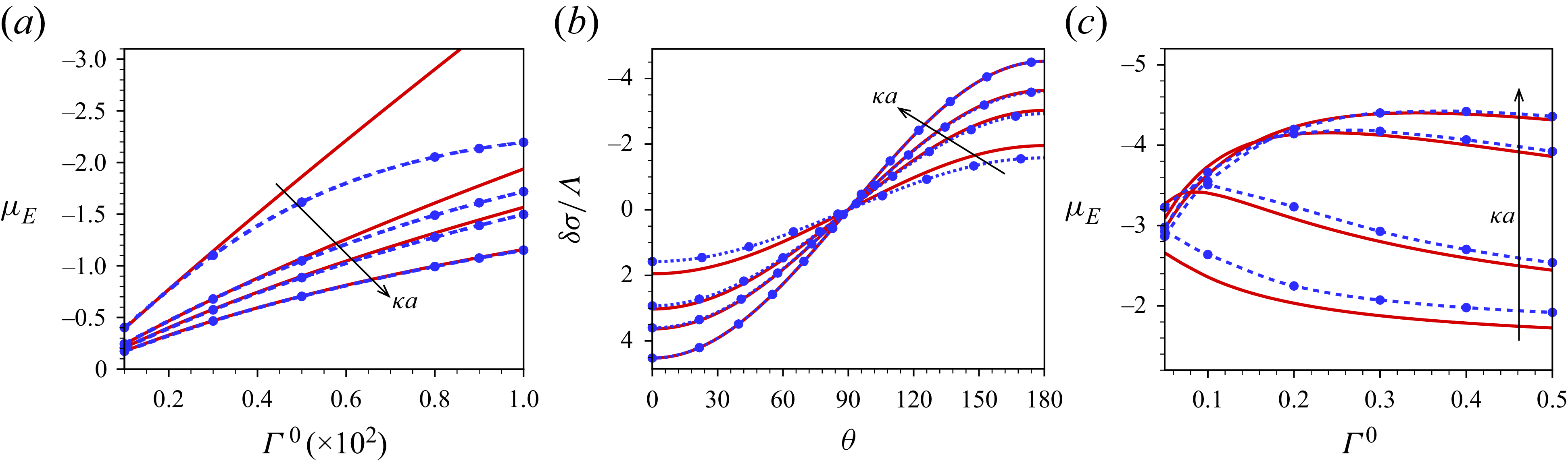
Figure 2. Variation of (a) electrophoretic mobility
 $\mu _{E}$
as a function of
$\mu _{E}$
as a function of
 $\varGamma ^{0}$
, (b) mobile surface charge density at the interface when
$\varGamma ^{0}$
, (b) mobile surface charge density at the interface when
 $\varGamma ^{0}=5\times 10^{-2}$
and (c)
$\varGamma ^{0}=5\times 10^{-2}$
and (c)
 $\mu _{E}$
as a function of
$\mu _{E}$
as a function of
 $\varGamma ^{0}$
. In (a,b), the viscosity ratio
$\varGamma ^{0}$
. In (a,b), the viscosity ratio
 $\mu _{r}=1$
,
$\mu _{r}=1$
,
 $\kappa a=1,5,10,50$
and
$\kappa a=1,5,10,50$
and
 $\varGamma ^{\infty }=1 \,\textrm{nm}^{-2}\ (Ma=876.61)$
. Red lines in (a) represent analytical expression (5.17), while in (b), they represent the analytical expression (5.26). In (c), the viscosity ratio
$\varGamma ^{\infty }=1 \,\textrm{nm}^{-2}\ (Ma=876.61)$
. Red lines in (a) represent analytical expression (5.17), while in (b), they represent the analytical expression (5.26). In (c), the viscosity ratio
 $\mu _{r}=0.1$
,
$\mu _{r}=0.1$
,
 $\kappa a=10,20,40,50$
,
$\kappa a=10,20,40,50$
,
 $\varGamma ^{\infty }=1 \,\textrm{nm}^{-2}\ (Ma=876.61)$
and red lines represent the analytical expression (5.53). In all panels, the blue lines with symbols represent the numerical solutions. All solutions are obtained for NaCl electrolyte.
$\varGamma ^{\infty }=1 \,\textrm{nm}^{-2}\ (Ma=876.61)$
and red lines represent the analytical expression (5.53). In all panels, the blue lines with symbols represent the numerical solutions. All solutions are obtained for NaCl electrolyte.
Figure 2(b) presents a comparison between the analytical and numerical solution for part of the surface charge density (
 $\delta \sigma$
) resulting from the non-uniform surfactant distribution. The analytical expression (5.26) exhibits slight deviations from the numerical simulation at smaller values of
$\delta \sigma$
) resulting from the non-uniform surfactant distribution. The analytical expression (5.26) exhibits slight deviations from the numerical simulation at smaller values of
 $\kappa a$
, primarily due to the relaxation effect. However, as
$\kappa a$
, primarily due to the relaxation effect. However, as
 $\kappa a$
increases, these deviations diminish, and the analytical solution aligns well with the numerical results. At higher values of
$\kappa a$
increases, these deviations diminish, and the analytical solution aligns well with the numerical results. At higher values of
 $\kappa a$
, the surface potential becomes lower than the thermal potential. Under these conditions, the Debye layer relaxation effects become negligible, resulting in an excellent agreement between the analytical solution and the numerical simulations.
$\kappa a$
, the surface potential becomes lower than the thermal potential. Under these conditions, the Debye layer relaxation effects become negligible, resulting in an excellent agreement between the analytical solution and the numerical simulations.
The mobility expression (5.53) based on the thin-layer analysis is validated with the numerical result for
 $\kappa a = 10, 20, 40, 50$
by varying
$\kappa a = 10, 20, 40, 50$
by varying
 $\varGamma ^{0}$
in figure 2(c). While the overall qualitative trends are identical, a slight deviation is observed for smaller values of
$\varGamma ^{0}$
in figure 2(c). While the overall qualitative trends are identical, a slight deviation is observed for smaller values of
 $\kappa a$
. This deviation arises because the analytical solution is based on a thin-Debye-layer consideration, which becomes less accurate at a lower
$\kappa a$
. This deviation arises because the analytical solution is based on a thin-Debye-layer consideration, which becomes less accurate at a lower
 $\kappa a$
.
$\kappa a$
.
6.2. Comparison of results based on the SEM with existing studies
In figure 3(a), we compare our numerical results based on the SEM with the analytical expression of Booth (Reference Booth1951) under the assumptions of immobile interfacial charge and no Marangoni stress. As demonstrated earlier in § 5.1.2, our analytical solution reduces to the expression derived by Booth (Reference Booth1951) under the Debye–Hückel approximation. Here, we observe that in the regime where the Debye–Hückel approximation holds, i.e. when
 $\sigma / (\kappa a + 1) \lt 1$
, our numerical results closely match with the analytical formula of Booth (Reference Booth1951). However, a deviation appears beyond this limit due to the occurrence of a significant double-layer polarisation effect, which is not accounted for in Booth (Reference Booth1951). Note that the expression of Booth (Reference Booth1951) is equivalent to that of Mahapatra et al. (Reference Mahapatra, Ohshima and Gopmandal2022) for non-conducting, non-polarisable droplets.
$\sigma / (\kappa a + 1) \lt 1$
, our numerical results closely match with the analytical formula of Booth (Reference Booth1951). However, a deviation appears beyond this limit due to the occurrence of a significant double-layer polarisation effect, which is not accounted for in Booth (Reference Booth1951). Note that the expression of Booth (Reference Booth1951) is equivalent to that of Mahapatra et al. (Reference Mahapatra, Ohshima and Gopmandal2022) for non-conducting, non-polarisable droplets.
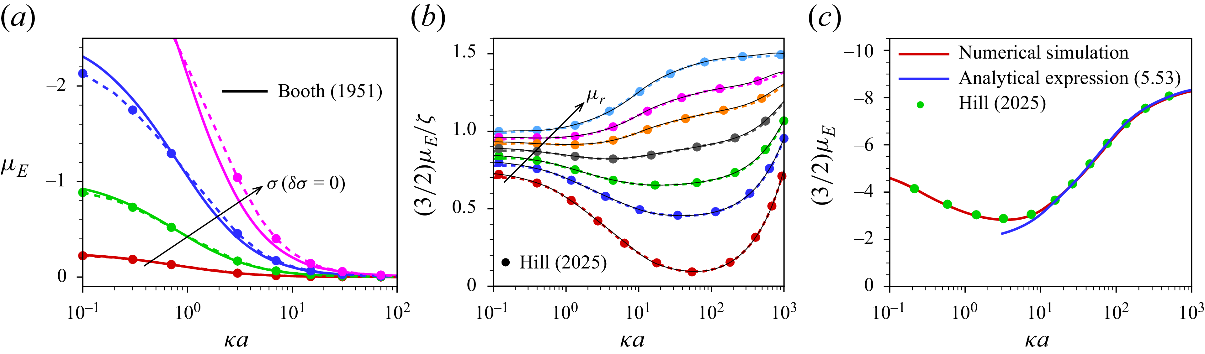
Figure 3. (a) Comparison of
 $\mu _E$
with the expression of Booth (Reference Booth1951) ((5.39)) as a function of
$\mu _E$
with the expression of Booth (Reference Booth1951) ((5.39)) as a function of
 $\kappa a$
for a non-polarisable, non-conducting droplet (
$\kappa a$
for a non-polarisable, non-conducting droplet (
 $\lambda =0.5$
). Solid lines, solution of Booth (Reference Booth1951); dashed lines, numerical results based on the present SEM for constant surface charge density and no Marangoni stress. The surface charge values
$\lambda =0.5$
). Solid lines, solution of Booth (Reference Booth1951); dashed lines, numerical results based on the present SEM for constant surface charge density and no Marangoni stress. The surface charge values
 $\sigma = -0.5$
,
$\sigma = -0.5$
,
 $-2$
,
$-2$
,
 $-5$
and
$-5$
and
 $-10$
correspond to
$-10$
correspond to
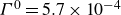 $\varGamma ^{0} = 5.7 \times 10^{-4}$
,
$\varGamma ^{0} = 5.7 \times 10^{-4}$
,
 $22.8 \times 10^{-4}$
,
$22.8 \times 10^{-4}$
,
 $57.1 \times 10^{-4}$
and
$57.1 \times 10^{-4}$
and
 $114.2 \times 10^{-4}$
, respectively, with
$114.2 \times 10^{-4}$
, respectively, with
 $\mu _r = 0.1$
and
$\mu _r = 0.1$
and
 $\varGamma ^\infty = 1\,\textrm{nm}^{-2}$
. (b) Comparison with Hill (Reference Hill2025) for non-polarisable droplets with mobile surface charge density
$\varGamma ^\infty = 1\,\textrm{nm}^{-2}$
. (b) Comparison with Hill (Reference Hill2025) for non-polarisable droplets with mobile surface charge density
 $\mu _{r}=0.001,0.25,0.5,1,2,4,10^{3}$
,
$\mu _{r}=0.001,0.25,0.5,1,2,4,10^{3}$
,
 $\zeta ^{0}=-0.001$
,
$\zeta ^{0}=-0.001$
,
 $D_{s}=10^{-6}\,\textrm{m}^{2}\textrm{s}^{-1}$
and
$D_{s}=10^{-6}\,\textrm{m}^{2}\textrm{s}^{-1}$
and
 $\varGamma ^{\infty }=1 \,\textrm{nm}^{-2}\ (Ma=876.61)$
. Circles, results taken from figure 1(a) of Hill (Reference Hill2025); solid black lines, present analytic solution (5.34); coloured dashed lines, computation from the present SEM neglecting the Marangoni stress. (c) Comparison with the figure 8(a) of Hill (Reference Hill2025) for a highly charged non-polarisable droplet with
$\varGamma ^{\infty }=1 \,\textrm{nm}^{-2}\ (Ma=876.61)$
. Circles, results taken from figure 1(a) of Hill (Reference Hill2025); solid black lines, present analytic solution (5.34); coloured dashed lines, computation from the present SEM neglecting the Marangoni stress. (c) Comparison with the figure 8(a) of Hill (Reference Hill2025) for a highly charged non-polarisable droplet with
 $\zeta ^{0}=-5$
and
$\zeta ^{0}=-5$
and
 $\mu _{r}=0.01$
. Here,
$\mu _{r}=0.01$
. Here,
 $a=50\,\textrm{nm}$
and
$a=50\,\textrm{nm}$
and
 $D_{s}=D^{\infty }_{2}=3.94\times 10^{-10}\,\textrm m^2\,{\textrm s}^{-1}$
. Symbols, Hill (Reference Hill2025) with
$D_{s}=D^{\infty }_{2}=3.94\times 10^{-10}\,\textrm m^2\,{\textrm s}^{-1}$
. Symbols, Hill (Reference Hill2025) with
 $k_{d}=0$
; red line, numerical results based on the SEM; blue line, analytical solution (5.53).
$k_{d}=0$
; red line, numerical results based on the SEM; blue line, analytical solution (5.53).
Figure 3(b) presents a comparison with figure 1(a) of Hill (Reference Hill2025) for mobile surface charge density but no Marangoni stress. For the computation,
 $\varGamma ^{0}$
is obtained through the relation
$\varGamma ^{0}$
is obtained through the relation
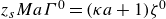 $z_{s}Ma\varGamma ^{0}=(\kappa a+1)\zeta ^{0}$
, valid for
$z_{s}Ma\varGamma ^{0}=(\kappa a+1)\zeta ^{0}$
, valid for
 $\zeta ^{0}\lt 1$
. We find that our analytical expression (5.34) as well as the numerical simulation perfectly match with the computed results of Hill (Reference Hill2025). In figure 3(b), comparisons are specifically made for droplets with very low
$\zeta ^{0}\lt 1$
. We find that our analytical expression (5.34) as well as the numerical simulation perfectly match with the computed results of Hill (Reference Hill2025). In figure 3(b), comparisons are specifically made for droplets with very low
 $\zeta ^{0}$
-potential and negligible Marangoni stress, covering viscosity ratios in the range of
$\zeta ^{0}$
-potential and negligible Marangoni stress, covering viscosity ratios in the range of
 $10^{-3}$
to
$10^{-3}$
to
 $10^{3}$
. Figure 3(c) further compares our results with those of Hill (Reference Hill2025) for droplets having high
$10^{3}$
. Figure 3(c) further compares our results with those of Hill (Reference Hill2025) for droplets having high
 $\zeta ^{0}$
-potential (
$\zeta ^{0}$
-potential (
 $\zeta ^{0}=-5$
), incorporating both interfacial charge mobility and Marangoni stress for a viscosity ratio
$\zeta ^{0}=-5$
), incorporating both interfacial charge mobility and Marangoni stress for a viscosity ratio
 $\mu _{r}=0.01$
based on the SEM. We find that our numerical results exactly match the results of Hill (Reference Hill2025) across the entire range of
$\mu _{r}=0.01$
based on the SEM. We find that our numerical results exactly match the results of Hill (Reference Hill2025) across the entire range of
 $\kappa a$
, as expected, given that both studies employ the same numerical approach. Remarkably, our thin-Debye-layer-based analytical expression (5.53) combined with (5.56) demonstrates exact agreement with numerical results of Hill (Reference Hill2025) for
$\kappa a$
, as expected, given that both studies employ the same numerical approach. Remarkably, our thin-Debye-layer-based analytical expression (5.53) combined with (5.56) demonstrates exact agreement with numerical results of Hill (Reference Hill2025) for
 $\kappa a\gt 10$
. Furthermore, as evidenced by figures 3(b) and 3(c), our analytical and numerical solutions are accurately valid for the entire range of
$\kappa a\gt 10$
. Furthermore, as evidenced by figures 3(b) and 3(c), our analytical and numerical solutions are accurately valid for the entire range of
 $\mu _{r}$
, confirming their applicability to bubbles (
$\mu _{r}$
, confirming their applicability to bubbles (
 $\mu _{r}\lt 0.1$
), droplets and rigid colloids (
$\mu _{r}\lt 0.1$
), droplets and rigid colloids (
 $\mu _{r}\to \infty$
). While these comparisons are for kinetic-exchange rate
$\mu _{r}\to \infty$
). While these comparisons are for kinetic-exchange rate
 $k_{d}=0$
, Hill (Reference Hill2025) studied the impact of kinetic-exchange and pointed out that it has a relatively weak influence on the mobility for a higher
$k_{d}=0$
, Hill (Reference Hill2025) studied the impact of kinetic-exchange and pointed out that it has a relatively weak influence on the mobility for a higher
 $\zeta ^{0}$
-potential.
$\zeta ^{0}$
-potential.
6.3. Droplet electrophoresis in monovalent electrolytes by different models
The variation of electrophoretic mobility of the droplet (
 $ \mu _E$
) as a function of the bulk ionic concentration (
$ \mu _E$
) as a function of the bulk ionic concentration (
 $\kappa a$
) is depicted in figure 4(a,b) for different droplet viscosity at a fixed Marangoni number and different equilibrium surfactant concentration
$\kappa a$
) is depicted in figure 4(a,b) for different droplet viscosity at a fixed Marangoni number and different equilibrium surfactant concentration
 $\varGamma ^0$
. The dashed lines correspond to the numerical results based on the SEM, while the solid lines represent the analytical solution derived from (5.53). For
$\varGamma ^0$
. The dashed lines correspond to the numerical results based on the SEM, while the solid lines represent the analytical solution derived from (5.53). For
 $\kappa a \gt 30$
, the numerical solutions based on the SEM align perfectly well with the analytical solution (5.53). Moreover, numerical results obtained with the MEMC show an insignificant difference compared with the SEM for
$\kappa a \gt 30$
, the numerical solutions based on the SEM align perfectly well with the analytical solution (5.53). Moreover, numerical results obtained with the MEMC show an insignificant difference compared with the SEM for
 $\kappa a \leqslant 110$
, corresponding to bulk molar concentrations up to
$\kappa a \leqslant 110$
, corresponding to bulk molar concentrations up to
 $ 115 \, \textrm{mM}$
. However, as
$ 115 \, \textrm{mM}$
. However, as
 $\kappa a$
exceeds 110, deviation between the SEM and MEMC become pronounced and this discrepancy increases with
$\kappa a$
exceeds 110, deviation between the SEM and MEMC become pronounced and this discrepancy increases with
 $\kappa a$
. Despite these quantitative differences, the pattern of variation of
$\kappa a$
. Despite these quantitative differences, the pattern of variation of
 $ \mu _E$
with
$ \mu _E$
with
 $\kappa a$
is similar for both models, with the MEMC determining slightly lower mobilities at a higher
$\kappa a$
is similar for both models, with the MEMC determining slightly lower mobilities at a higher
 $\kappa a$
. This reduction in
$\kappa a$
. This reduction in
 $-\mu _E$
under the MEMC arises as the electrostatic ion–ion correlations enhance the shielding effect by drawing more counterions into the vicinity of the charged surface. In addition, the modified model accounts for an increased electrolyte viscosity near the droplet, which results in greater viscous friction as well as lower ionic mobility. Together, these factors contribute to the observed reduction in
$-\mu _E$
under the MEMC arises as the electrostatic ion–ion correlations enhance the shielding effect by drawing more counterions into the vicinity of the charged surface. In addition, the modified model accounts for an increased electrolyte viscosity near the droplet, which results in greater viscous friction as well as lower ionic mobility. Together, these factors contribute to the observed reduction in
 $-\mu _{E}$
by the MEMC compared with the SEM.
$-\mu _{E}$
by the MEMC compared with the SEM.
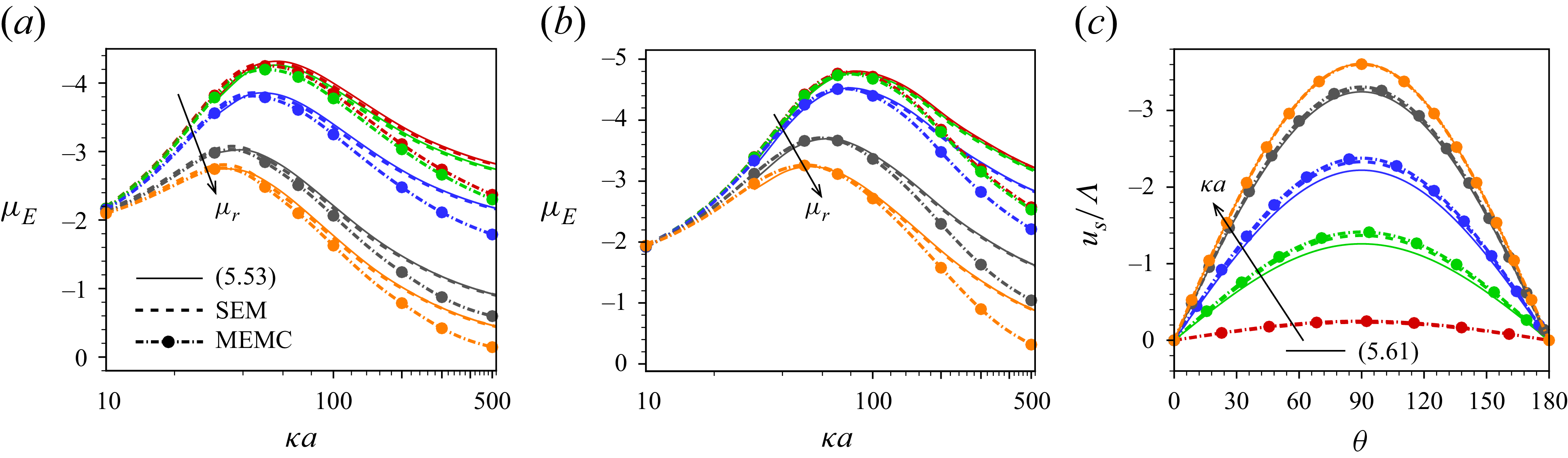
Figure 4. Variation of electrophoretic mobility
 $\mu _{E}$
as a function of
$\mu _{E}$
as a function of
 $\kappa a$
at (a)
$\kappa a$
at (a)
 $\varGamma ^{0}=0.2$
and (b)
$\varGamma ^{0}=0.2$
and (b)
 $\varGamma ^{0}=0.4$
for
$\varGamma ^{0}=0.4$
for
 $\mu _{r}=0.1,1,10,100,1000$
and (c) interface velocity
$\mu _{r}=0.1,1,10,100,1000$
and (c) interface velocity
 $u_{s}$
at
$u_{s}$
at
 $\varGamma ^{0}=0.4$
for different
$\varGamma ^{0}=0.4$
for different
 $\kappa a\ (=10,30,50,100,200)$
for
$\kappa a\ (=10,30,50,100,200)$
for
 $\mu _{r}=0.1$
. Here,
$\mu _{r}=0.1$
. Here,
 $\textit{Ma}=10^{3}$
. Solid lines, analytical solutions based on SEM for (a,b)
$\textit{Ma}=10^{3}$
. Solid lines, analytical solutions based on SEM for (a,b)
 $\mu _E$
(5.53) and (c)
$\mu _E$
(5.53) and (c)
 $u_{s}$
(5.61); dashed lines, SEM; dash-dotted lines, MEMC.
$u_{s}$
(5.61); dashed lines, SEM; dash-dotted lines, MEMC.
Figure 4(a,b) reveals a non-monotonic dependence of
 $\mu _E$
on
$\mu _E$
on
 $ \kappa a$
. Specifically,
$ \kappa a$
. Specifically,
 $|\mu _E|$
increases with
$|\mu _E|$
increases with
 $ \kappa a$
, reaching a local maximum at a critical
$ \kappa a$
, reaching a local maximum at a critical
 $ \kappa a$
, then decreases with further increases in
$ \kappa a$
, then decreases with further increases in
 $ \kappa a$
. The critical
$ \kappa a$
. The critical
 $\kappa a$
at which the maximum in
$\kappa a$
at which the maximum in
 $|\mu _{E}|$
occurs becomes higher for lower viscosity ratio
$|\mu _{E}|$
occurs becomes higher for lower viscosity ratio
 $(\mu _r)$
and higher equilibrium surfactant concentration
$(\mu _r)$
and higher equilibrium surfactant concentration
 $( \varGamma ^0 )$
. This non-monotonic behaviour of
$( \varGamma ^0 )$
. This non-monotonic behaviour of
 $\mu _{E}$
with
$\mu _{E}$
with
 $\kappa a$
arises due to the interplay between three key factors as
$\kappa a$
arises due to the interplay between three key factors as
 $\kappa a$
increases, namely: (i) a reduction in surface conduction, which contributes to enhancing
$\kappa a$
increases, namely: (i) a reduction in surface conduction, which contributes to enhancing
 $-\mu _{E}$
, (ii) a decrease in surface potential, which tends to reduce
$-\mu _{E}$
, (ii) a decrease in surface potential, which tends to reduce
 $-\mu _{E}$
, and (iii) an enhancement in interfacial velocity (figure 4
c) at the droplet surface contributing to the enhancement of
$-\mu _{E}$
, and (iii) an enhancement in interfacial velocity (figure 4
c) at the droplet surface contributing to the enhancement of
 $-\mu _{E}$
. At a lower
$-\mu _{E}$
. At a lower
 $ \kappa a$
, the reduction in surface conduction and the increase in interface velocity dominate, leading to an overall increase in
$ \kappa a$
, the reduction in surface conduction and the increase in interface velocity dominate, leading to an overall increase in
 $- \mu _E$
. However, with further increases of
$- \mu _E$
. However, with further increases of
 $ \kappa a$
, the diminishing surface potential becomes the dominant factor, causing
$ \kappa a$
, the diminishing surface potential becomes the dominant factor, causing
 $-\mu _E$
to decline. For this reason, a non-monotonic pattern in
$-\mu _E$
to decline. For this reason, a non-monotonic pattern in
 $\mu _{E}$
occurs as
$\mu _{E}$
occurs as
 $\kappa a$
(or the bulk concentration of the electrolyte) is varied.
$\kappa a$
(or the bulk concentration of the electrolyte) is varied.
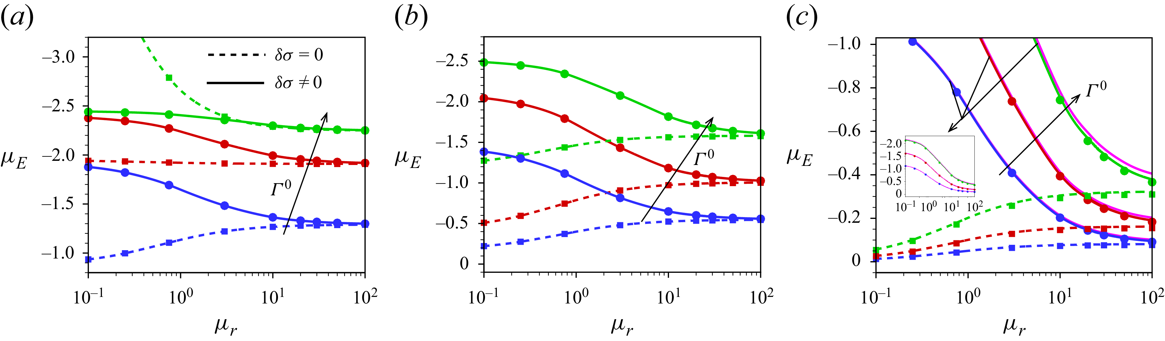
Figure 5. Variation of electrophoretic mobility
 $\mu _{E}$
as a function of viscosity ratio
$\mu _{E}$
as a function of viscosity ratio
 $\mu _{r}$
at (a)
$\mu _{r}$
at (a)
 $\kappa a=1$
, (b)
$\kappa a=1$
, (b)
 $\kappa a=5$
and (c)
$\kappa a=5$
and (c)
 $\kappa a=50$
for various
$\kappa a=50$
for various
 $\varGamma ^{0}=0.005,0.01,0.02$
(blue, red and green lines, respectively) at
$\varGamma ^{0}=0.005,0.01,0.02$
(blue, red and green lines, respectively) at
 $\varGamma ^{\infty }=1 \,\textrm{nm}^{-2}\ (Ma=876.61)$
. Solid lines correspond to the droplet with compressible surfactants (
$\varGamma ^{\infty }=1 \,\textrm{nm}^{-2}\ (Ma=876.61)$
. Solid lines correspond to the droplet with compressible surfactants (
 $\delta \sigma \neq 0$
), while dashed lines represent a uniformly charged droplet (
$\delta \sigma \neq 0$
), while dashed lines represent a uniformly charged droplet (
 $\delta \sigma = 0$
). Circles, MEMC (
$\delta \sigma = 0$
). Circles, MEMC (
 $\delta \sigma \neq 0$
); squares, MEMC (
$\delta \sigma \neq 0$
); squares, MEMC (
 $\delta \sigma =0$
); and in (c) pink lines, Smoluchowski mobility based on (5.29). Inset of (c) shows
$\delta \sigma =0$
); and in (c) pink lines, Smoluchowski mobility based on (5.29). Inset of (c) shows
 $\mu _{E}$
versus
$\mu _{E}$
versus
 $\mu _{r}$
for
$\mu _{r}$
for
 $\delta \sigma \neq 0$
at different
$\delta \sigma \neq 0$
at different
 $\varGamma ^{0}$
.
$\varGamma ^{0}$
.
Figure 4(c) shows that the tangential velocity
 $u_{s}$
at the surface of the droplet enhances as
$u_{s}$
at the surface of the droplet enhances as
 $\kappa a$
is increased and this increase in
$\kappa a$
is increased and this increase in
 $u_{s}$
is significant for a low-viscosity droplet. The analytical expression (5.61) shows an excellent agreement with the numerical results for
$u_{s}$
is significant for a low-viscosity droplet. The analytical expression (5.61) shows an excellent agreement with the numerical results for
 $\kappa a\gt 30$
. We find that the effect of the finite size of ions and the correlations among ions on the interface velocity is negligible. With the increase of
$\kappa a\gt 30$
. We find that the effect of the finite size of ions and the correlations among ions on the interface velocity is negligible. With the increase of
 $\kappa a$
, the hydrodynamic stress enhances the interface velocity and, hence, the internal circulation within the droplet. This increase in interfacial velocity, in turn, contributes to the augmentation of the liquid-phase component of
$\kappa a$
, the hydrodynamic stress enhances the interface velocity and, hence, the internal circulation within the droplet. This increase in interfacial velocity, in turn, contributes to the augmentation of the liquid-phase component of
 $\mu _{E}$
. Figure 5 illustrates the variation of droplet mobility as a function of viscosity ratio
$\mu _{E}$
. Figure 5 illustrates the variation of droplet mobility as a function of viscosity ratio
 $\mu _{r}$
for different values of the equilibrium surfactant concentration
$\mu _{r}$
for different values of the equilibrium surfactant concentration
 $\varGamma ^{0}$
and Debye-layer thickness. Previous studies (Wu et al. Reference Wu, Fan, Jian and Lee2021; Rashidi, Zargartalebi & Benneker Reference Rashidi, Zargartalebi and Benneker2021) on the electrophoresis of a dielectric droplet with uniform surface charge density (
$\varGamma ^{0}$
and Debye-layer thickness. Previous studies (Wu et al. Reference Wu, Fan, Jian and Lee2021; Rashidi, Zargartalebi & Benneker Reference Rashidi, Zargartalebi and Benneker2021) on the electrophoresis of a dielectric droplet with uniform surface charge density (
 $\delta \sigma =0$
) has shown that
$\delta \sigma =0$
) has shown that
 $\mu _{E}$
may enhance with the increase of
$\mu _{E}$
may enhance with the increase of
 $\mu _{r}$
for certain range of
$\mu _{r}$
for certain range of
 $\kappa a$
and surface charge density,
$\kappa a$
and surface charge density,
 $\varGamma ^{0}$
. In figure 5, the dashed lines represent such a scenario where the surfactant concentration is uniform, i.e. the Marangoni stress is absent (
$\varGamma ^{0}$
. In figure 5, the dashed lines represent such a scenario where the surfactant concentration is uniform, i.e. the Marangoni stress is absent (
 $\delta \sigma = 0$
). Under these conditions,
$\delta \sigma = 0$
). Under these conditions,
 $|\mu _E|$
increases with
$|\mu _E|$
increases with
 $\mu _r$
at low values of
$\mu _r$
at low values of
 $\varGamma ^0$
, while it decreases for higher
$\varGamma ^0$
, while it decreases for higher
 $\varGamma ^0$
when
$\varGamma ^0$
when
 $\kappa a = 1$
. For higher values of
$\kappa a = 1$
. For higher values of
 $\kappa a$
,
$\kappa a$
,
 $|\mu _E|$
increases with
$|\mu _E|$
increases with
 $\mu _r$
monotonically. However, this trend changes when Marangoni stress is included (
$\mu _r$
monotonically. However, this trend changes when Marangoni stress is included (
 $\delta \sigma \neq 0$
), as shown by the solid lines. In this case,
$\delta \sigma \neq 0$
), as shown by the solid lines. In this case,
 $|\mu _E|$
decreases with increasing
$|\mu _E|$
decreases with increasing
 $\mu _r$
. This numerical finding is corroborated by the analytical solutions (5.23) and (5.57), which explicitly show that
$\mu _r$
. This numerical finding is corroborated by the analytical solutions (5.23) and (5.57), which explicitly show that
 $|\mu _E|$
is a decreasing function of
$|\mu _E|$
is a decreasing function of
 $\mu _r$
when Marangoni stress is considered. When the surfactant concentration is uniform (i.e. no Marangoni stress), the flow field within the droplet is governed by the interaction of hydrodynamic and Maxwell stresses at the interface. The Maxwell stress spins the droplet in the opposite direction to the electrophoresis of the droplet. This results in formation of a recirculating toroidal vortex at the outer side of the droplet surface, which slows down the electrophoretic mobility and its impact is significant at a lower
$\mu _r$
when Marangoni stress is considered. When the surfactant concentration is uniform (i.e. no Marangoni stress), the flow field within the droplet is governed by the interaction of hydrodynamic and Maxwell stresses at the interface. The Maxwell stress spins the droplet in the opposite direction to the electrophoresis of the droplet. This results in formation of a recirculating toroidal vortex at the outer side of the droplet surface, which slows down the electrophoretic mobility and its impact is significant at a lower
 $\mu _{r}$
. For this
$\mu _{r}$
. For this
 $|\mu _{E}|$
increases with
$|\mu _{E}|$
increases with
 $\mu _{r}$
when
$\mu _{r}$
when
 $\delta \sigma = 0$
. It is evident from figure 6(a,b) that the internal circulation
$\delta \sigma = 0$
. It is evident from figure 6(a,b) that the internal circulation
 $\varOmega$
is counterclockwise and
$\varOmega$
is counterclockwise and
 $u_s$
is positive, but
$u_s$
is positive, but
 $\mu _E \lt 0$
(figure 5
b) for
$\mu _E \lt 0$
(figure 5
b) for
 $\delta \sigma = 0$
. As
$\delta \sigma = 0$
. As
 $\mu _r$
increases, this vortex shrinks, allowing the droplet to move faster, leading to an enhancement in mobility with increasing
$\mu _r$
increases, this vortex shrinks, allowing the droplet to move faster, leading to an enhancement in mobility with increasing
 $\mu _r$
.
$\mu _r$
.
When a non-uniform surfactant concentration is present (
 $\delta \sigma \neq 0$
), a non-zero surface tension gradient introduces Marangoni stress into the interfacial stress balance condition. The Marangoni stress has two origins: one arising from electromigration and the other from convection. The electromigration component counteracts the tangential Maxwell stress at the interface, leaving the flow field in the drop region primarily driven by hydrodynamic stress and the convective component of the Marangoni stress of surfactant. This results in the interfacial velocity along the direction of flow outside the droplet, i.e.
$\delta \sigma \neq 0$
), a non-zero surface tension gradient introduces Marangoni stress into the interfacial stress balance condition. The Marangoni stress has two origins: one arising from electromigration and the other from convection. The electromigration component counteracts the tangential Maxwell stress at the interface, leaving the flow field in the drop region primarily driven by hydrodynamic stress and the convective component of the Marangoni stress of surfactant. This results in the interfacial velocity along the direction of flow outside the droplet, i.e.
 $u_{s}\lt 0$
. With increasing
$u_{s}\lt 0$
. With increasing
 $\mu _{r}$
, the mobility
$\mu _{r}$
, the mobility
 $|\mu _{E}|$
decreases, which causes the internal circulation to diminish, as shown in figure 6(a,b).
$|\mu _{E}|$
decreases, which causes the internal circulation to diminish, as shown in figure 6(a,b).
Figure 6(c) depicts the distribution of the non-uniform part of the surface charge density
 $\delta \sigma$
created by
$\delta \sigma$
created by
 $\delta \varGamma$
as the Debye-layer thickness
$\delta \varGamma$
as the Debye-layer thickness
 $\kappa a$
is varied. The surface charge density on the droplet arises from the adsorption of surfactant molecules at the interface. Under the influence of an external electric field, the surfactant molecules become non-uniformly distributed along the interface. We find that
$\kappa a$
is varied. The surface charge density on the droplet arises from the adsorption of surfactant molecules at the interface. Under the influence of an external electric field, the surfactant molecules become non-uniformly distributed along the interface. We find that
 $\delta \sigma$
becomes higher for higher values of
$\delta \sigma$
becomes higher for higher values of
 $\kappa a$
.
$\kappa a$
.

Figure 6. Variation of (a) internal circulation strength (
 $\varOmega$
) as a function of
$\varOmega$
) as a function of
 $\mu _{r}$
at
$\mu _{r}$
at
 $\kappa a=5$
and (b) interface velocity at
$\kappa a=5$
and (b) interface velocity at
 $\kappa a=5$
and
$\kappa a=5$
and
 $\mu _{r}=0.1$
for various
$\mu _{r}=0.1$
for various
 $\varGamma ^{0}=0.005,0.01,0.02$
(shown as blue, red and green lines, respectively). (c) Mobile surface charge density
$\varGamma ^{0}=0.005,0.01,0.02$
(shown as blue, red and green lines, respectively). (c) Mobile surface charge density
 $\delta \sigma$
at
$\delta \sigma$
at
 $\varGamma ^{0}=0.01$
and
$\varGamma ^{0}=0.01$
and
 $\mu _{r}=0.1$
for different
$\mu _{r}=0.1$
for different
 $\kappa a=1,5,50$
(blue, red and green lines, respectively). Here,
$\kappa a=1,5,50$
(blue, red and green lines, respectively). Here,
 $\varGamma ^{\infty }=1 \,\textrm{nm}^{-2}\ (Ma=876.61)$
. Circles, MEMC (
$\varGamma ^{\infty }=1 \,\textrm{nm}^{-2}\ (Ma=876.61)$
. Circles, MEMC (
 $\delta \sigma \neq 0$
); squares, MEMC (
$\delta \sigma \neq 0$
); squares, MEMC (
 $\delta \sigma =0$
).
$\delta \sigma =0$
).

Figure 7. Variation of (a)
 $\mu _{E}$
and (b)
$\mu _{E}$
and (b)
 $\varPsi (1)$
(radial part of the perturbed electric potential) as a function of
$\varPsi (1)$
(radial part of the perturbed electric potential) as a function of
 $\varGamma ^{0}$
when
$\varGamma ^{0}$
when
 $\kappa a=50$
and
$\kappa a=50$
and
 $\varGamma ^{\infty }=1 \,\textrm{nm}^{-2}\ (Ma=876.61)$
. (c) Electrophoretic mobility
$\varGamma ^{\infty }=1 \,\textrm{nm}^{-2}\ (Ma=876.61)$
. (c) Electrophoretic mobility
 $\mu _{E}$
as a function of
$\mu _{E}$
as a function of
 $\textit{Ma}$
for various
$\textit{Ma}$
for various
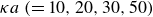 $\kappa a\ (=10,20,30,50)$
with
$\kappa a\ (=10,20,30,50)$
with
 $\varGamma ^{0}=0.3$
. Here,
$\varGamma ^{0}=0.3$
. Here,
 $\mu _{r}=0.1$
. In (a), pink solid line, analytical expression (5.53). Circles, MEMC (
$\mu _{r}=0.1$
. In (a), pink solid line, analytical expression (5.53). Circles, MEMC (
 $\delta \sigma\neq0$
); squares, MEMC (
$\delta \sigma\neq0$
); squares, MEMC (
 $\delta \sigma =0$
).
$\delta \sigma =0$
).
Figure 7(a) shows the variation of the mobility with equilibrium surfactant concentration
 $\varGamma ^{0}$
, assuming both a uniform surface charge density (
$\varGamma ^{0}$
, assuming both a uniform surface charge density (
 $\delta \sigma =0$
) as well as a non-uniform surfactant distribution (
$\delta \sigma =0$
) as well as a non-uniform surfactant distribution (
 $\delta \sigma \neq 0$
). We find that for the case of a uniformly charged surface,
$\delta \sigma \neq 0$
). We find that for the case of a uniformly charged surface,
 $\mu _{E}$
increases with
$\mu _{E}$
increases with
 $\varGamma ^{0}$
, then undergoes a jump discontinuity and ultimately becomes negative. Several authors (Schnitzer et al. Reference Schnitzer, Frankel and Yariv2014; Wu et al. Reference Wu, Fan, Jian and Lee2021) have encountered a jump discontinuity in
$\varGamma ^{0}$
, then undergoes a jump discontinuity and ultimately becomes negative. Several authors (Schnitzer et al. Reference Schnitzer, Frankel and Yariv2014; Wu et al. Reference Wu, Fan, Jian and Lee2021) have encountered a jump discontinuity in
 $\mu _{E}$
when varied with the uniform surface charge density for higher values of
$\mu _{E}$
when varied with the uniform surface charge density for higher values of
 $\kappa a$
. In those studies they adopted the SEM and failed to provide an explanation on the occurrence of this jump discontinuity in
$\kappa a$
. In those studies they adopted the SEM and failed to provide an explanation on the occurrence of this jump discontinuity in
 $\mu _{E}$
. In order to gain insight into this phenomenon, we have presented the radial part of the perturbed surface potential
$\mu _{E}$
. In order to gain insight into this phenomenon, we have presented the radial part of the perturbed surface potential
 $\varPsi (1)$
(figure 7
b) by varying
$\varPsi (1)$
(figure 7
b) by varying
 $\varGamma ^{0}$
for both uniform (
$\varGamma ^{0}$
for both uniform (
 $\delta \sigma =0$
) as well as non-uniform (
$\delta \sigma =0$
) as well as non-uniform (
 $\delta \sigma \neq 0$
) surface charge. It may be noted that
$\delta \sigma \neq 0$
) surface charge. It may be noted that
 $\varPsi (1)$
measures the Maxwell traction (
$\varPsi (1)$
measures the Maxwell traction (
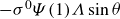 $-\sigma ^{0}\varPsi (1)\varLambda \sin \theta$
) at the interface for a fixed
$-\sigma ^{0}\varPsi (1)\varLambda \sin \theta$
) at the interface for a fixed
 $\sigma ^{0}$
. It is evident that
$\sigma ^{0}$
. It is evident that
 $\varPsi (1)$
becomes unboundedly large for the range of
$\varPsi (1)$
becomes unboundedly large for the range of
 $\varGamma ^{0}$
for which
$\varGamma ^{0}$
for which
 $\mu _{E}$
encounters a jump discontinuity when
$\mu _{E}$
encounters a jump discontinuity when
 $\delta \sigma =0$
, i.e. for the case of uniform surfactant distribution. Obviously, the weak-field analysis based on the first-order perturbation technique ceases to remain valid where
$\delta \sigma =0$
, i.e. for the case of uniform surfactant distribution. Obviously, the weak-field analysis based on the first-order perturbation technique ceases to remain valid where
 $\varPsi (1)$
becomes unboundedly large. However, the variation in
$\varPsi (1)$
becomes unboundedly large. However, the variation in
 $\mu _{E}$
as well as
$\mu _{E}$
as well as
 $\varPsi (1)$
with
$\varPsi (1)$
with
 $\varGamma ^{0}$
is found to be smooth when
$\varGamma ^{0}$
is found to be smooth when
 $\delta \sigma \neq 0$
. Based on the weak-field analysis we find that a non-uniform distribution of ionic surfactant creates a smooth variation of
$\delta \sigma \neq 0$
. Based on the weak-field analysis we find that a non-uniform distribution of ionic surfactant creates a smooth variation of
 $\varPsi (1)$
, leading to a continuous dependence of the Maxwell traction on
$\varPsi (1)$
, leading to a continuous dependence of the Maxwell traction on
 $\varGamma ^{0}$
. Hill (Reference Hill2025) also concluded that when the interfacial charge is considered to be mobile, a continuous mobility arises even in the absence of Marangoni effects. We have seen (not presented here for the sake of brevity) that the mobility has a smooth dependence on
$\varGamma ^{0}$
. Hill (Reference Hill2025) also concluded that when the interfacial charge is considered to be mobile, a continuous mobility arises even in the absence of Marangoni effects. We have seen (not presented here for the sake of brevity) that the mobility has a smooth dependence on
 $\varGamma ^{0}$
for the non-uniform surfactant distribution (
$\varGamma ^{0}$
for the non-uniform surfactant distribution (
 $\delta \sigma \neq 0$
) even when the Marangoni effect is neglected in the boundary condition (3.33). However,
$\delta \sigma \neq 0$
) even when the Marangoni effect is neglected in the boundary condition (3.33). However,
 $\mu _{E}$
differs once the Marangoni effect is excluded from the boundary condition (3.33). We may thus conclude that the singularity observed in
$\mu _{E}$
differs once the Marangoni effect is excluded from the boundary condition (3.33). We may thus conclude that the singularity observed in
 $\mu _{E}$
at a higher range of constant surface charge density is an artefact of the idealised immobile surface charge assumption compounded by the breakdown of the weak-field approximation at high surface coverage. The analytical expression (5.53) for
$\mu _{E}$
at a higher range of constant surface charge density is an artefact of the idealised immobile surface charge assumption compounded by the breakdown of the weak-field approximation at high surface coverage. The analytical expression (5.53) for
 $\mu _{E}$
also yields a smooth dependence on
$\mu _{E}$
also yields a smooth dependence on
 $\varGamma ^{0}$
.
$\varGamma ^{0}$
.
Figure 7(c) illustrates the impact of the Marangoni number (
 $\textit{Ma}$
) on the mobility (
$\textit{Ma}$
) on the mobility (
 $\mu _{E}$
) for various values of
$\mu _{E}$
) for various values of
 $\kappa a$
at
$\kappa a$
at
 $\varGamma ^{0} = 0.3$
for a low-viscosity droplet. The Marangoni number influences both the charge distribution at the droplet interface as well as the Marangoni stress. The results indicate a significant enhancement in
$\varGamma ^{0} = 0.3$
for a low-viscosity droplet. The Marangoni number influences both the charge distribution at the droplet interface as well as the Marangoni stress. The results indicate a significant enhancement in
 $|\mu _{E}|$
with increasing
$|\mu _{E}|$
with increasing
 $\textit{Ma}$
up to a moderate range for all values of
$\textit{Ma}$
up to a moderate range for all values of
 $\kappa a$
. For a higher range of
$\kappa a$
. For a higher range of
 $\textit{Ma}$
, the mobility reduces with the increase of
$\textit{Ma}$
, the mobility reduces with the increase of
 $\textit{Ma}$
for a lower
$\textit{Ma}$
for a lower
 $\kappa a$
, whereas
$\kappa a$
, whereas
 $|\mu _{E}|$
increases with
$|\mu _{E}|$
increases with
 $\textit{Ma}$
when
$\textit{Ma}$
when
 $\kappa a$
is higher. The interface potential generally enhances mobility, while surface conduction and Marangoni stress tend to reduce it. At a lower range of
$\kappa a$
is higher. The interface potential generally enhances mobility, while surface conduction and Marangoni stress tend to reduce it. At a lower range of
 $\textit{Ma}$
, both surface conduction and Marangoni stress remain weak, allowing
$\textit{Ma}$
, both surface conduction and Marangoni stress remain weak, allowing
 $|\mu _{E}|$
to increase rapidly with the increase of
$|\mu _{E}|$
to increase rapidly with the increase of
 $\textit{Ma}$
due to the enhancement of interface potential. However, as
$\textit{Ma}$
due to the enhancement of interface potential. However, as
 $\textit{Ma}$
increases, the effects of surface conduction and Marangoni stress amplify, which inhibits the rapid enhancement of
$\textit{Ma}$
increases, the effects of surface conduction and Marangoni stress amplify, which inhibits the rapid enhancement of
 $|\mu _{E}|$
. For lower
$|\mu _{E}|$
. For lower
 $\kappa a$
, surface conduction and Marangoni stress dominate, leading to a decrease in
$\kappa a$
, surface conduction and Marangoni stress dominate, leading to a decrease in
 $|\mu _{E}|$
with an increase of
$|\mu _{E}|$
with an increase of
 $\textit{Ma}$
for the higher range of
$\textit{Ma}$
for the higher range of
 $\textit{Ma}$
. In contrast, at larger
$\textit{Ma}$
. In contrast, at larger
 $\kappa a$
, surface conduction and Marangoni stress weaken, and despite a reduction in interface potential,
$\kappa a$
, surface conduction and Marangoni stress weaken, and despite a reduction in interface potential,
 $|\mu _{E}|$
continues to increase, albeit at a diminishing rate.
$|\mu _{E}|$
continues to increase, albeit at a diminishing rate.

Figure 8. Variation of
 $\mu _{E}$
at (a)
$\mu _{E}$
at (a)
 $\kappa a=50$
and (b)
$\kappa a=50$
and (b)
 $\kappa a=100$
and variation of internal circulation strength at (c)
$\kappa a=100$
and variation of internal circulation strength at (c)
 $\kappa a=100$
as a function of
$\kappa a=100$
as a function of
 $\varGamma ^{0}$
for various
$\varGamma ^{0}$
for various
 $\mu _{r}=0.1,1,10,100,1000$
and
$\mu _{r}=0.1,1,10,100,1000$
and
 $\varGamma ^{\infty }=1 \,\textrm{nm}^{-2}\ (Ma=876.61)$
. Solid lines, analytical solution of (a,b) mobility (5.53) and (c) internal circulation strength (5.62); dashed lines, SEM; circles, MEMC.
$\varGamma ^{\infty }=1 \,\textrm{nm}^{-2}\ (Ma=876.61)$
. Solid lines, analytical solution of (a,b) mobility (5.53) and (c) internal circulation strength (5.62); dashed lines, SEM; circles, MEMC.
The influence of equilibrium surfactant concentration
 $\varGamma ^{0}$
on the mobility
$\varGamma ^{0}$
on the mobility
 $\mu _{E}$
and the internal circulation strength
$\mu _{E}$
and the internal circulation strength
 $\varOmega$
is analysed in figure 8 for a fixed Marangoni number
$\varOmega$
is analysed in figure 8 for a fixed Marangoni number
 $\textit{Ma}$
. Figure 8(a) demonstrates that
$\textit{Ma}$
. Figure 8(a) demonstrates that
 $|\mu _E|$
increases rapidly with
$|\mu _E|$
increases rapidly with
 $\varGamma ^{0}$
at its lower values. This rate of increase slows down when
$\varGamma ^{0}$
at its lower values. This rate of increase slows down when
 $\varGamma ^{0}$
is increased further. Eventually, the mobility attains a saturation at higher values of
$\varGamma ^{0}$
is increased further. Eventually, the mobility attains a saturation at higher values of
 $\varGamma ^{0}$
and the critical value of
$\varGamma ^{0}$
and the critical value of
 $\varGamma ^{0}$
for which the saturation in
$\varGamma ^{0}$
for which the saturation in
 $\mu _{E}$
occurs is lower for a low-viscosity droplet. This behaviour arises because increasing
$\mu _{E}$
occurs is lower for a low-viscosity droplet. This behaviour arises because increasing
 $\varGamma ^{0}$
elevates the surface charge density, which enhances the surface potential of the droplet, thereby amplifying
$\varGamma ^{0}$
elevates the surface charge density, which enhances the surface potential of the droplet, thereby amplifying
 $\mu _{E}$
. However, as the surface potential rises, Debye-layer polarisation manifests, which exerts a retardation effect that becomes progressively stronger, ultimately leading to a mobility saturation at a sufficiently large
$\mu _{E}$
. However, as the surface potential rises, Debye-layer polarisation manifests, which exerts a retardation effect that becomes progressively stronger, ultimately leading to a mobility saturation at a sufficiently large
 $\varGamma ^{0}$
. A saturation in mobility for a low-viscosity droplet when varying the constant surface charge density (i.e. in the absence of Marangoni stress) is attributed to the stronger retardation forces due to enhanced surface conduction (Majhi & Bhattacharyya Reference Majhi and Bhattacharyya2024). A higher
$\varGamma ^{0}$
. A saturation in mobility for a low-viscosity droplet when varying the constant surface charge density (i.e. in the absence of Marangoni stress) is attributed to the stronger retardation forces due to enhanced surface conduction (Majhi & Bhattacharyya Reference Majhi and Bhattacharyya2024). A higher
 $\varGamma ^{0}$
amplifies the Marangoni stress, further contributing to the observed saturation behaviour. In contrast, figure 8(b) shows that for
$\varGamma ^{0}$
amplifies the Marangoni stress, further contributing to the observed saturation behaviour. In contrast, figure 8(b) shows that for
 $\kappa a = 100$
,
$\kappa a = 100$
,
 $|\mu _E|$
continues to increase with
$|\mu _E|$
continues to increase with
 $\varGamma ^{0}$
but follows a slightly different qualitative pattern. No saturation in
$\varGamma ^{0}$
but follows a slightly different qualitative pattern. No saturation in
 $|\mu _{E}|$
is observed for the considered range of
$|\mu _{E}|$
is observed for the considered range of
 $\varGamma ^{0}$
, as at higher
$\varGamma ^{0}$
, as at higher
 $\kappa a$
the impact of double-layer polarisation diminishes.
$\kappa a$
the impact of double-layer polarisation diminishes.
Figure 8(c) shows that the internal circulation strength
 $\varOmega$
enhances with
$\varOmega$
enhances with
 $\varGamma ^{0}$
and attains a saturation for a low-viscosity droplet. As
$\varGamma ^{0}$
and attains a saturation for a low-viscosity droplet. As
 $\varGamma ^{0}$
increases, the surface potential rises, enhancing the hydrodynamic stress at the interface and thereby increasing the velocity of the flow within the droplet’s interior, leading to an increase in
$\varGamma ^{0}$
increases, the surface potential rises, enhancing the hydrodynamic stress at the interface and thereby increasing the velocity of the flow within the droplet’s interior, leading to an increase in
 $\varOmega$
. Much like mobility,
$\varOmega$
. Much like mobility,
 $\varOmega$
eventually saturates for low-viscosity droplets due to the combined effects of high surface conduction and Marangoni stress. The increase in Marangoni stress with
$\varOmega$
eventually saturates for low-viscosity droplets due to the combined effects of high surface conduction and Marangoni stress. The increase in Marangoni stress with
 $\varGamma ^{0}$
creates a stabilising effect that limits further enhancement of
$\varGamma ^{0}$
creates a stabilising effect that limits further enhancement of
 $\varOmega$
.
$\varOmega$
.
6.4. Droplet electrophoresis in multivalent electrolyte solutions by the MEMC
As indicated in § 1, for a multivalent electrolyte with high surface charge density, the electrostatic coupling parameter becomes large enough so that the correlation among ions becomes strong. Unless otherwise specified, we consider electrophoresis in an LaCl
 $_3$
electrolyte solution and equilibrium surfactant concentration
$_3$
electrolyte solution and equilibrium surfactant concentration
 $\varGamma ^{0}$
large enough to create a high surface charge density. A comparison of the mobility obtained by the SEM and MEMC for electrophoresis in a trivalent electrolyte is provided and discussed in Appendix B (figure 13
b). The results presented in this section are obtained based on the MEMC. We begin by comparing the mobility (
$\varGamma ^{0}$
large enough to create a high surface charge density. A comparison of the mobility obtained by the SEM and MEMC for electrophoresis in a trivalent electrolyte is provided and discussed in Appendix B (figure 13
b). The results presented in this section are obtained based on the MEMC. We begin by comparing the mobility (
 $\mu _E$
) obtained by using our proposed boundary condition, BC-1 (2.9), i.e.
$\mu _E$
) obtained by using our proposed boundary condition, BC-1 (2.9), i.e.
 $\boldsymbol{t}\boldsymbol{\cdot }{{\nabla} }^{3}\psi =0$
, with results based on the frequently adopted boundary condition, i.e. BC-2,
$\boldsymbol{t}\boldsymbol{\cdot }{{\nabla} }^{3}\psi =0$
, with results based on the frequently adopted boundary condition, i.e. BC-2,
 $\boldsymbol{n}\boldsymbol{\cdot }{{\nabla} }^{3}\psi =0$
(Bazant et al. Reference Bazant, Storey and Kornyshev2011), as depicted in figure 9(a). To ensure accuracy, the comparison is performed for various electrolyte solutions and bulk ionic concentrations. The results reveal that the difference in mobility obtained by BC-1 (2.9) and BC-2 is negligible, highlighting the consistency of our proposed boundary condition with the established one.
$\boldsymbol{n}\boldsymbol{\cdot }{{\nabla} }^{3}\psi =0$
(Bazant et al. Reference Bazant, Storey and Kornyshev2011), as depicted in figure 9(a). To ensure accuracy, the comparison is performed for various electrolyte solutions and bulk ionic concentrations. The results reveal that the difference in mobility obtained by BC-1 (2.9) and BC-2 is negligible, highlighting the consistency of our proposed boundary condition with the established one.
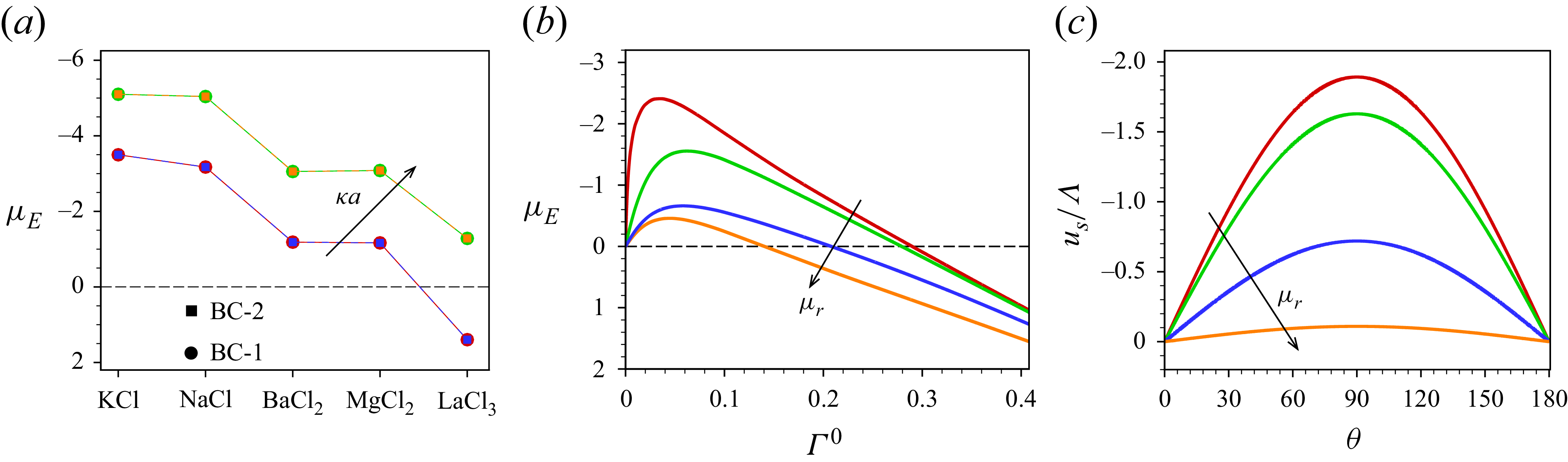
Figure 9. Variation of mobility (a) for different electrolyte solutions at
 $\kappa a=30\text{ and }100$
when
$\kappa a=30\text{ and }100$
when
 $\mu _{r}=0.1$
and
$\mu _{r}=0.1$
and
 $\varGamma ^{0}=0.3$
and (b) as a function of
$\varGamma ^{0}=0.3$
and (b) as a function of
 $\varGamma ^{0}$
for various
$\varGamma ^{0}$
for various
 $\mu _{r}\ (=0.1,10,100,1000)$
at
$\mu _{r}\ (=0.1,10,100,1000)$
at
 $\kappa a=50$
. (c) Interface velocity for various
$\kappa a=50$
. (c) Interface velocity for various
 $\mu _{r}\ (=0.1,10,100,1000)$
at
$\mu _{r}\ (=0.1,10,100,1000)$
at
 $\kappa a=50$
and
$\kappa a=50$
and
 $\varGamma ^{0}=0.2$
. In (a), BC-1 is
$\varGamma ^{0}=0.2$
. In (a), BC-1 is
 $\boldsymbol{t}\boldsymbol{\cdot }{{\nabla} }^{3}\psi =0$
((2.9)) and BC-2 is
$\boldsymbol{t}\boldsymbol{\cdot }{{\nabla} }^{3}\psi =0$
((2.9)) and BC-2 is
 $\boldsymbol{n}\boldsymbol{\cdot }{{\nabla} }^{3}\psi =0$
and in (b,c) we have taken LaCl
$\boldsymbol{n}\boldsymbol{\cdot }{{\nabla} }^{3}\psi =0$
and in (b,c) we have taken LaCl
 $_3$
as electrolyte. Here, we have taken
$_3$
as electrolyte. Here, we have taken
 $\varGamma ^{\infty }=2\,\textrm{nm}^{-2}$
(
$\varGamma ^{\infty }=2\,\textrm{nm}^{-2}$
(
 $\textit{Ma}=1753.2$
).
$\textit{Ma}=1753.2$
).
The ion–ion correlations enhance the concentration of counterions in the vicinity of a charged surface due to the strong electrostatic coupling in a trivalent electrolyte. These counterions form a densely adsorbed layer, referred to as the counterion condensed layer, which overcompensates the surface charge. This overcompensation leads to an attraction of coions into the EDL to maintain charge neutrality. This process may result in an oscillation in polarity of the charge density as well as in electric potential, as depicted in figure 10(a,b). These effects cause mobility reversal in rigid colloids (
 $\mu _{r} \to \infty$
), as demonstrated in existing studies (Semenov et al. Reference Semenov, Raafatnia, Sega, Lobaskin, Holm and Kremer2013; Stout & Khair Reference Stout and Khair2014; Paik et al. Reference Paik, Bhattacharyya and Majhi2024). However, in droplets, the dynamics becomes significantly different owing to the interface velocity and mobility of the interface charge.
$\mu _{r} \to \infty$
), as demonstrated in existing studies (Semenov et al. Reference Semenov, Raafatnia, Sega, Lobaskin, Holm and Kremer2013; Stout & Khair Reference Stout and Khair2014; Paik et al. Reference Paik, Bhattacharyya and Majhi2024). However, in droplets, the dynamics becomes significantly different owing to the interface velocity and mobility of the interface charge.
Figure 9(b) illustrates the variation of mobility,
 $\mu _{E}$
, as a function of
$\mu _{E}$
, as a function of
 $\varGamma ^{0}$
, for droplets with different viscosity ratios
$\varGamma ^{0}$
, for droplets with different viscosity ratios
 $\mu _{r}$
, at
$\mu _{r}$
, at
 $\kappa a =50$
. The results exhibit a non-monotonic trend, where
$\kappa a =50$
. The results exhibit a non-monotonic trend, where
 $-\mu _{E}$
increases with
$-\mu _{E}$
increases with
 $\varGamma ^{0}$
in its lower range, then it decreases and reverses direction from positive to negative as
$\varGamma ^{0}$
in its lower range, then it decreases and reverses direction from positive to negative as
 $\varGamma ^{0}$
is further increased. This reversal in mobility is strongly influenced by the droplet viscosity. For droplets with low
$\varGamma ^{0}$
is further increased. This reversal in mobility is strongly influenced by the droplet viscosity. For droplets with low
 $\mu _{r}$
, the mobility reversal is delayed, while for high-viscosity droplets, the reversal occurs at comparatively lower surfactant concentration. At lower values of
$\mu _{r}$
, the mobility reversal is delayed, while for high-viscosity droplets, the reversal occurs at comparatively lower surfactant concentration. At lower values of
 $\varGamma ^{0}$
, the ion–ion correlation effects and Marangoni stress are relatively weak, leading to an increase in
$\varGamma ^{0}$
, the ion–ion correlation effects and Marangoni stress are relatively weak, leading to an increase in
 $\mu _{E}$
with
$\mu _{E}$
with
 $\varGamma ^{0}$
. This increase is more pronounced for droplets with lower
$\varGamma ^{0}$
. This increase is more pronounced for droplets with lower
 $\mu _{r}$
, where the interfacial velocity is stronger. The interfacial velocity as presented in figure 9(c) shows that it is higher for droplets with lower
$\mu _{r}$
, where the interfacial velocity is stronger. The interfacial velocity as presented in figure 9(c) shows that it is higher for droplets with lower
 $\mu _{r}$
. However, as
$\mu _{r}$
. However, as
 $\varGamma ^{0}$
increases, the combined effect of enhanced Marangoni stress, surface conduction and stronger shielding effect due to ion correlations reduces
$\varGamma ^{0}$
increases, the combined effect of enhanced Marangoni stress, surface conduction and stronger shielding effect due to ion correlations reduces
 $-\mu _{E}$
. At a sufficiently high
$-\mu _{E}$
. At a sufficiently high
 $\varGamma ^{0}$
, the dominance of ion correlations leads to a reversal in mobility. This transition is further elucidated in subsequent discussion by presenting the spatial distribution of charge density and electric potential.
$\varGamma ^{0}$
, the dominance of ion correlations leads to a reversal in mobility. This transition is further elucidated in subsequent discussion by presenting the spatial distribution of charge density and electric potential.

Figure 10. Variation of (a)
 $\overline {\rho }_{e}$
and (b) electric potential at
$\overline {\rho }_{e}$
and (b) electric potential at
 $\theta =\pi /2$
for
$\theta =\pi /2$
for
 $\mu _{r}=0.1$
and
$\mu _{r}=0.1$
and
 $\varGamma ^{0}=0.05,0.1,0.2,0.3, 0.4$
. In (a,b),
$\varGamma ^{0}=0.05,0.1,0.2,0.3, 0.4$
. In (a,b),
 $\varGamma ^{\infty }=2\,\textrm{nm}^{-2}$
(
$\varGamma ^{\infty }=2\,\textrm{nm}^{-2}$
(
 $\textit{Ma}=1753.2$
) and
$\textit{Ma}=1753.2$
) and
 $\kappa a=50$
; electrolyte is LaCl
$\kappa a=50$
; electrolyte is LaCl
 $_3$
. Arrow in the inset of figure 10(b) is along the decreasing direction of
$_3$
. Arrow in the inset of figure 10(b) is along the decreasing direction of
 $\varGamma ^{0}$
. (c) Variation of
$\varGamma ^{0}$
. (c) Variation of
 $\mu _{E}$
as a function of
$\mu _{E}$
as a function of
 $\textit{Ma}$
at
$\textit{Ma}$
at
 $\kappa a=50$
,
$\kappa a=50$
,
 $\varGamma ^{0}=0.3$
and
$\varGamma ^{0}=0.3$
and
 $\mu _{r}=0.1$
for different electrolyte salts (KCl, BaCl
$\mu _{r}=0.1$
for different electrolyte salts (KCl, BaCl
 $_2$
, LaCl
$_2$
, LaCl
 $_3$
).
$_3$
).

Figure 11. Variation of (a)
 $\mu _{E}$
as a function of
$\mu _{E}$
as a function of
 $\textit{Ma}$
, (b) interface velocity at
$\textit{Ma}$
, (b) interface velocity at
 $\textit{Ma}=5000$
for
$\textit{Ma}=5000$
for
 $\mu _{r}=0.1$
and
$\mu _{r}=0.1$
and
 $\varGamma ^{0}=0.2$
and (c)
$\varGamma ^{0}=0.2$
and (c)
 $\mu _{E}$
as a function of viscosity ratio
$\mu _{E}$
as a function of viscosity ratio
 $\mu _{r}$
at
$\mu _{r}$
at
 $\varGamma ^{0}=0.3$
when
$\varGamma ^{0}=0.3$
when
 $\varGamma ^{\infty }=2\,\textrm{nm}^{-2}\ (Ma=1753.2)$
. Here,
$\varGamma ^{\infty }=2\,\textrm{nm}^{-2}\ (Ma=1753.2)$
. Here,
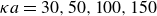 $\kappa a=30,50,100,150$
and electrolyte is LaCl
$\kappa a=30,50,100,150$
and electrolyte is LaCl
 $_3$
.
$_3$
.
Figure 10(a) illustrates the average space charge density, defined as
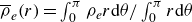 $\overline {\rho }_{e}(r) = \int _{0}^{\pi } \rho _{e} r {\textrm d}\theta / \int _{0}^{\pi } r {\textrm d}\theta$
, for different values of
$\overline {\rho }_{e}(r) = \int _{0}^{\pi } \rho _{e} r {\textrm d}\theta / \int _{0}^{\pi } r {\textrm d}\theta$
, for different values of
 $\varGamma ^{0}$
for the case of a low-viscosity droplet. The results indicate the formation of a condensed layer of counterions near the interface, followed by a sharp decrease in
$\varGamma ^{0}$
for the case of a low-viscosity droplet. The results indicate the formation of a condensed layer of counterions near the interface, followed by a sharp decrease in
 $\overline {\rho }_{e}(r)$
and eventually a reversal in polarity of the charge density. This reversal becomes pronounced with increasing
$\overline {\rho }_{e}(r)$
and eventually a reversal in polarity of the charge density. This reversal becomes pronounced with increasing
 $\varGamma ^{0}$
, corroborating the inversion in polarity of the electric potential observed in figure 10(b). These findings substantiate the previously discussed mobility reversal at higher
$\varGamma ^{0}$
, corroborating the inversion in polarity of the electric potential observed in figure 10(b). These findings substantiate the previously discussed mobility reversal at higher
 $\varGamma ^{0}$
.
$\varGamma ^{0}$
.
Figure 10(c) illustrates the variation of electrophoretic mobility (
 $\mu _{E}$
) as a function of the Marangoni number (
$\mu _{E}$
) as a function of the Marangoni number (
 $\textit{Ma}$
) for three electrolyte solutions, namely monovalent (KCl), divalent (BaCl
$\textit{Ma}$
) for three electrolyte solutions, namely monovalent (KCl), divalent (BaCl
 $_2$
) and trivalent (LaCl
$_2$
) and trivalent (LaCl
 $_3$
), in a low-viscosity droplet at a moderate surface coverage (
$_3$
), in a low-viscosity droplet at a moderate surface coverage (
 $\varGamma ^{0} = 0.3$
). The results show that the mobility reversal is found for the electrolyte with trivalent counterions, while no such reversal in mobility is seen for the monovalent or divalent electrolyte solutions. The impact of the electrostatic correlations depends on the scaled correlation length,
$\varGamma ^{0} = 0.3$
). The results show that the mobility reversal is found for the electrolyte with trivalent counterions, while no such reversal in mobility is seen for the monovalent or divalent electrolyte solutions. The impact of the electrostatic correlations depends on the scaled correlation length,
 $\delta _{c}$
, which depends on the counterion valency (
$\delta _{c}$
, which depends on the counterion valency (
 $V_{c}$
). For monovalent (
$V_{c}$
). For monovalent (
 $V_{c}=1$
) and divalent (
$V_{c}=1$
) and divalent (
 $V_{c}=2$
) electrolytes,
$V_{c}=2$
) electrolytes,
 $\delta _{c}$
remains significantly lower than in the trivalent (
$\delta _{c}$
remains significantly lower than in the trivalent (
 $V_{c}=3$
) case. For instance, at
$V_{c}=3$
) case. For instance, at
 $\kappa a = 50$
,
$\kappa a = 50$
,
 $\varGamma ^{0} = 0.3$
and
$\varGamma ^{0} = 0.3$
and
 $\textit{Ma} = 2000$
,
$\textit{Ma} = 2000$
,
 $\delta _{c}$
is 0.453, 0.307 and 0.158 for trivalent, divalent and monovalent electrolytes, respectively. Consequently, electrostatic correlations in monovalent and divalent electrolytes are not strong enough to cause mobility reversal. A similar trend has been observed for rigid colloids (Kubíčková et al. Reference Kubíčková, Křížek, Coufal, Vazdar, Wernersson, Heyda and Jungwirth2012; Semenov et al. Reference Semenov, Raafatnia, Sega, Lobaskin, Holm and Kremer2013).
$\delta _{c}$
is 0.453, 0.307 and 0.158 for trivalent, divalent and monovalent electrolytes, respectively. Consequently, electrostatic correlations in monovalent and divalent electrolytes are not strong enough to cause mobility reversal. A similar trend has been observed for rigid colloids (Kubíčková et al. Reference Kubíčková, Křížek, Coufal, Vazdar, Wernersson, Heyda and Jungwirth2012; Semenov et al. Reference Semenov, Raafatnia, Sega, Lobaskin, Holm and Kremer2013).
Figure 11(a) illustrates the variation of the mobility
 $\mu _{E}$
as a function of the Marangoni number (
$\mu _{E}$
as a function of the Marangoni number (
 $\textit{Ma}$
) for different values of
$\textit{Ma}$
) for different values of
 $\kappa a$
, considering a low-viscosity droplet with a fixed equilibrium surfactant concentration
$\kappa a$
, considering a low-viscosity droplet with a fixed equilibrium surfactant concentration
 $\varGamma ^{0}$
. The Marangoni number, in conjunction with the surfactant concentration, specifies the surface charge at the interface, which increases with
$\varGamma ^{0}$
. The Marangoni number, in conjunction with the surfactant concentration, specifies the surface charge at the interface, which increases with
 $\textit{Ma}$
. Simultaneously,
$\textit{Ma}$
. Simultaneously,
 $\textit{Ma}$
amplifies the effects of the Marangoni stress. As shown in figure 11(a),
$\textit{Ma}$
amplifies the effects of the Marangoni stress. As shown in figure 11(a),
 $\mu _{E}$
is negative at a lower
$\mu _{E}$
is negative at a lower
 $\textit{Ma}$
and
$\textit{Ma}$
and
 $-\mu _{E}$
increases with
$-\mu _{E}$
increases with
 $\textit{Ma}$
, reaching a critical value where
$\textit{Ma}$
, reaching a critical value where
 $\mu _{E}$
attains a peak for all considered values of
$\mu _{E}$
attains a peak for all considered values of
 $\kappa a$
. Beyond this critical
$\kappa a$
. Beyond this critical
 $\textit{Ma}$
,
$\textit{Ma}$
,
 $-\mu _{E}$
begins to decrease and
$-\mu _{E}$
begins to decrease and
 $\mu _{E}$
eventually becomes positive for increasingly larger values of
$\mu _{E}$
eventually becomes positive for increasingly larger values of
 $\textit{Ma}$
for a higher
$\textit{Ma}$
for a higher
 $\kappa a$
. At a low
$\kappa a$
. At a low
 $\textit{Ma}$
, the surface charge is moderate, leading to weaker ion–ion correlations and weaker surface conduction. For this,
$\textit{Ma}$
, the surface charge is moderate, leading to weaker ion–ion correlations and weaker surface conduction. For this,
 $\mu _{E}$
is negative and
$\mu _{E}$
is negative and
 $-\mu _{E}$
increases as
$-\mu _{E}$
increases as
 $\textit{Ma}$
enhances up to a critical value. Beyond this critical
$\textit{Ma}$
enhances up to a critical value. Beyond this critical
 $\textit{Ma}$
, which depends on
$\textit{Ma}$
, which depends on
 $\kappa a$
, electrostatic correlations become significant due to the enhanced surface charge density. These cause a reduction in
$\kappa a$
, electrostatic correlations become significant due to the enhanced surface charge density. These cause a reduction in
 $-\mu _{E}$
, eventually a change of sign of
$-\mu _{E}$
, eventually a change of sign of
 $\mu _{E}$
from negative to positive. The critical
$\mu _{E}$
from negative to positive. The critical
 $\textit{Ma}$
at which this reversal occurs increases with
$\textit{Ma}$
at which this reversal occurs increases with
 $\kappa a$
. At a higher
$\kappa a$
. At a higher
 $\kappa a$
, the interfacial velocity becomes significant, as shown in figure 11(b), which delays the flow reversal by imparting larger positive momentum to the liquid adjacent to the interface. Simultaneously, the impact of correlations diminishes due to a reduction in the interfacial electric potential. A lower interfacial potential suppresses oscillations in space charge density as fewer counterions and coions accumulate in the EDL, resulting in mobility remaining negative.
$\kappa a$
, the interfacial velocity becomes significant, as shown in figure 11(b), which delays the flow reversal by imparting larger positive momentum to the liquid adjacent to the interface. Simultaneously, the impact of correlations diminishes due to a reduction in the interfacial electric potential. A lower interfacial potential suppresses oscillations in space charge density as fewer counterions and coions accumulate in the EDL, resulting in mobility remaining negative.
Figure 11(c) depicts the variation of mobility
 $\mu _{E}$
with the viscosity ratio
$\mu _{E}$
with the viscosity ratio
 $\mu _{r}$
for different values of
$\mu _{r}$
for different values of
 $\kappa a$
at a fixed Marangoni number, considering an equilibrium surfactant concentration
$\kappa a$
at a fixed Marangoni number, considering an equilibrium surfactant concentration
 $\varGamma ^{0} = 0.3$
in an LaCl
$\varGamma ^{0} = 0.3$
in an LaCl
 $_3$
electrolyte solution. Results indicate that
$_3$
electrolyte solution. Results indicate that
 $|\mu _{E}|$
decreases with
$|\mu _{E}|$
decreases with
 $\mu _{r}$
when
$\mu _{r}$
when
 $\mu _{E} \lt 0$
, while it increases with
$\mu _{E} \lt 0$
, while it increases with
 $\mu _{r}$
when
$\mu _{r}$
when
 $\mu _{E} \gt 0$
. When
$\mu _{E} \gt 0$
. When
 $\mu _{E}$
is negative, no outer vortex develops and the adjacent flows just inside and outside of the droplet interface align in the same direction, similar to the behaviour observed in monovalent electrolytes. Consequently,
$\mu _{E}$
is negative, no outer vortex develops and the adjacent flows just inside and outside of the droplet interface align in the same direction, similar to the behaviour observed in monovalent electrolytes. Consequently,
 $|\mu _{E}|$
decreases with increasing
$|\mu _{E}|$
decreases with increasing
 $\mu _{r}$
under these conditions. The reversal in mobility arises due to the accumulation of coions within the EDL, which reverses the outer flow direction from positive to negative while the interfacial flow and the internal vortex retain the same sign. This reversal creates a vortex just outside the droplet, as shown in figure 12(b), creating a retarding force. This retarding force causes
$\mu _{r}$
under these conditions. The reversal in mobility arises due to the accumulation of coions within the EDL, which reverses the outer flow direction from positive to negative while the interfacial flow and the internal vortex retain the same sign. This reversal creates a vortex just outside the droplet, as shown in figure 12(b), creating a retarding force. This retarding force causes
 $\mu _{E}$
to become an increasing function of
$\mu _{E}$
to become an increasing function of
 $\mu _{r}$
. Interestingly, it is observed that
$\mu _{r}$
. Interestingly, it is observed that
 $\mu _{E}$
is positive across all values of
$\mu _{E}$
is positive across all values of
 $\mu _{r}$
for lower
$\mu _{r}$
for lower
 $\kappa a$
, where correlation effects dominate, but as
$\kappa a$
, where correlation effects dominate, but as
 $\kappa a$
increases the interface flow intensifies owing to enhanced convection in the surfactant distribution, delaying the reversal for the lower range of
$\kappa a$
increases the interface flow intensifies owing to enhanced convection in the surfactant distribution, delaying the reversal for the lower range of
 $\mu _{r}$
.
$\mu _{r}$
.
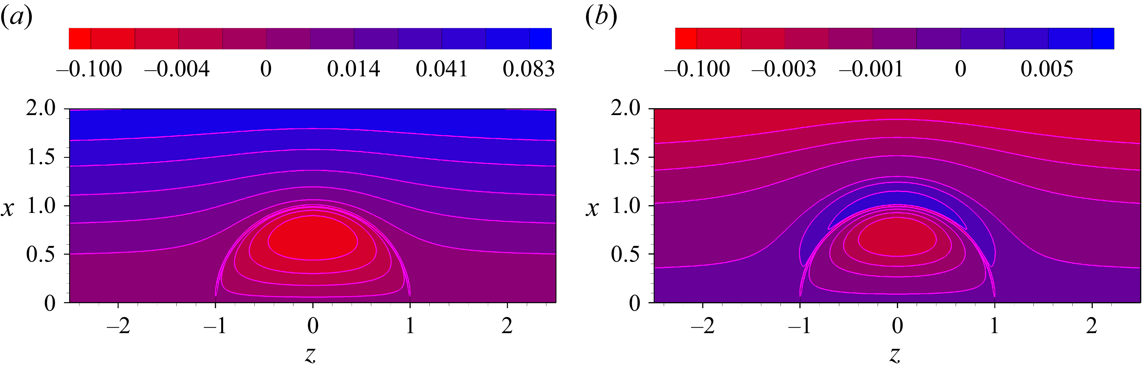
Figure 12. Streamlines at (a)
 $\mu _{r}=10$
and (b)
$\mu _{r}=10$
and (b)
 $\mu _{r}=200$
at
$\mu _{r}=200$
at
 $\kappa a=100$
and
$\kappa a=100$
and
 $\varGamma ^{0}=0.3$
. Here,
$\varGamma ^{0}=0.3$
. Here,
 $\varGamma ^{\infty }=2\,\textrm{nm}^{-2}$
(
$\varGamma ^{\infty }=2\,\textrm{nm}^{-2}$
(
 $\textit{Ma}=1753.2$
) and
$\textit{Ma}=1753.2$
) and
 $\varLambda =0.04$
. Electrolyte is LaCl
$\varLambda =0.04$
. Electrolyte is LaCl
 $_3$
.
$_3$
.
Figure 12 illustrates the streamline patterns inside and outside the droplet for a low-viscosity droplet (figure 12 a) and a high-viscosity droplet (figure 12 b), under a fixed equilibrium surfactant concentration and Marangoni number. The stream function describing the flow field can be obtained as
 \begin{equation} \nu (r,\theta ) = \begin{cases} \dfrac {1}{2}\dfrac {{\textrm d}\mathcal{H}}{{\textrm d}r}(1)r^{2}(1-r^{2})\varLambda \sin ^{2}\theta & \text{if } r \leqslant 1, \\[6pt] -r\mathcal{H}(r)\varLambda \sin ^{2}\theta & \text{if } r \gt 1. \end{cases} \end{equation}
Previous studies on droplet electrophoresis have reported vortex formation on the droplet surface by the flow adjacent to the interface of the droplet in both monovalent and multivalent electrolytes caused by the Maxwell traction imposed by the interfacial boundary condition. However, as discussed earlier, the Marangoni stress counteracts the tangential electric stress at the interface. Consequently, no vortices form due to the Maxwell traction, and the flow pattern resembles typical Stokes flow as depicted in figure 12(a). As discussed previously, for higher-viscosity or highly charged droplets in a trivalent electrolyte, ion correlations lead to a mobility reversal. This reversal is attributed to the reversed direction of the outer flow, while the internal flow direction remains unchanged. As a result, the flow adjacent to the droplet interface changes direction, creating a re-circulating vortex adjacent to the outer interface of the droplet as demonstrated in figure 12(b). Thus, the outer vortex emerges when the electrostatic correlations are strong enough to create an inversion in mobility direction, and it is observed in higher-viscosity droplets. For low-viscosity droplets, an enhanced interfacial flow compensates the momentum loss created by the coion-dominated layer induced by electrostatic correlations, leading to a suppression of mobility reversal.
7. Conclusion and outlook
This study investigates the electrophoresis of a non-polarizable, viscous droplet coated with irreversibly adsorbed ionic surfactants, suspended in monovalent or multivalent electrolytes. The surfactant concentration at the droplet interface is determined based on the Langmuir isotherm model. The surface charge of the droplet arises due to the adsorbed surfactants. The interface condition is governed by the balance of Marangoni stress, Maxwell stress and hydrodynamic stress. A modified electrokinetic model is adopted, which incorporates ion steric interactions and correlations of finite-sized ions, which ensures its validity for arbitrary surface potentials and bulk molar concentrations. The governing coupled set of equations are solved using a perturbation method under a weak applied electric field consideration, valid for an arbitrary interface potential and Debye-layer thickness. Based on the SEM, in which ions are considered as point charge and correlations between ions are neglected, we have derived analytical solutions for droplet electrophoresis in monovalent electrolytes under the Debye–Hückel approximation as well as the thin-EDL consideration.
We demonstrate that the mobility of a droplet laden with an insoluble ionic surfactant consistently decreases with increasing droplet-to-electrolyte viscosity ratio in monovalent electrolytes. This behaviour arises due to the counteraction between the Marangoni stress and tangential Maxwell stress. When a non-uniform distribution of surfactants is considered, the tangential electric stress at the droplet interface remains bounded and it varies continuously with the variation of surfactant concentration creating the droplet mobility to vary smoothly. Hill (Reference Hill2025) based on numerical simulation of the SEM also demonstrated a continuous variation of the droplet mobility with surface charge density when the mobility of interfacial charge is accounted for. Our analytical solution, derived under the SEM with a thin-Debye-layer assumption, complements this finding. A non-monotonic relationship between the droplet mobility and bulk ionic concentration is demonstrated through both analytical and numerical solutions. We find that in monovalent electrolytes, the mobility obtained by the MEMC is significantly lower than that obtained using the SEM at larger values of
 $\kappa a$
due to the occurrence of enhanced viscosity of the electrolyte.
$\kappa a$
due to the occurrence of enhanced viscosity of the electrolyte.
One of the key contributions of this study is to incorporate the effects of electrostatic correlations (MEMC) among finite-sized ions in the electrophoresis of surfactant-laden droplets. This elucidates the mechanisms of droplet mobility reversal in multivalent electrolytes, as found in existing experimental studies. The overcompensation of surface charge by multivalent counterions changes the polarity of the charge density in the EDL, thereby promoting mobility reversal, while the interfacial velocity acts in opposition, delaying or preventing the reversal entirely. In particular, the stronger interfacial velocity for low-viscosity droplets defers the mobility reversal induced by electrostatic correlations by creating an enhanced convection of the counterions in the condensed layer. Furthermore, we demonstrated that in situations where the mobility reverses direction, it may become an increasing function of the droplet-to-electrolyte viscosity ratio, due to induced vortices in the outer flow field near the droplet surface, generating a retarding force that counteracts its motion.
The modified model presented in this study can also be adapted to investigate related transport phenomena such as diffusiophoresis, thermophoresis and sedimentation of surfactant-laden droplets. The present model can be extended to include dynamic adsorption–desorption of ionic surfactant for a more generalised electrokinetic framework which accounts for ion saturation due to steric interactions and correlations among finite-sized ions. While this study focuses on weak electric fields, the framework provides a foundation for future investigations into strong-field regimes.
Funding
Financial support from the Anusandhan National Research Foundation (ANRF), Government of India (grant no. CRG/2022/005758) is gratefully acknowledged.
Declaration of interests
The authors report no conflict of interest.
Appendix A. Detailed derivation of equation (5.53)
To understand the approximations leading to (5.53), we first derive expressions for
 $\varPhi _\pm (1)$
. Abbreviating the integrals from (5.51) and (5.52) as
$\varPhi _\pm (1)$
. Abbreviating the integrals from (5.51) and (5.52) as
 \begin{align} \mathcal{I}_1(\zeta ^0; z_i) &= \int _0^{\zeta ^0} \frac {\beta (\psi ^{0};z_{i})}{\text{sgn}(\zeta ^{0})\chi (\psi ^0)} \, {\textrm d}\psi ^0, \end{align}
 \begin{align} \mathcal{I}_2(\zeta ^{0};z_{i}) &={\int _{0}^{\zeta ^{0}}\int _{\psi ^{0}}^{\zeta ^{0}} \frac {\beta (\psi ^{0};z_{i})}{\chi (\psi ^0)\chi ({\psi ^0}')}\,{\textrm d}{\psi ^{0}}'\,{\textrm d}\psi ^{0} }, \end{align}
 \begin{align} \mathcal{I}_3(\zeta ^{0}; z_i, z_j) &= \int _{0}^{\zeta ^{0}}\int _{\zeta ^{0}}^{\psi ^{0}}\int _{0}^{{\psi ^{0}}'}\frac {\beta (\psi ^{0};z_{i})\beta ({\psi ^{0}}'';z_{j})}{\text{sgn}(\zeta ^{0})\chi (\psi ^{0})\chi ({\psi ^{0}}')\chi ({\psi ^{0}}'')}\,{\textrm d}{\psi ^{0}}''\,{\textrm d}{\psi ^{0}}'\,{\textrm d}\psi ^{0}, \end{align}
with
 $\chi (\psi _0) = 2\sinh ({\psi ^0}/{2})\,\text{sgn}(\zeta ^{0})$
, one gets
$\chi (\psi _0) = 2\sinh ({\psi ^0}/{2})\,\text{sgn}(\zeta ^{0})$
, one gets
 \begin{align} \mathcal{I}_1(\zeta ^{0}; \pm 1) &= 2 \left (e^{\mp \zeta ^{0}/2} - 1\right )\!, \end{align}
 \begin{align} \mathcal{I}_2(\zeta ^{0}; \pm 1) &= 4\ln \left (\frac {1+e^{{\mp }{\zeta ^{0}/2}}}{2}\right )\!, \end{align}
 \begin{align} \mathcal{I}_3(\zeta ^{0}; z_i, z_i)\big |_{z_i = \pm 1} &= 8 \left [ \left (1 - e^{\mp \zeta ^{0}/2}\right ) + 2 \ln \left ( \frac {1+e^{\mp \zeta ^{0}/2}}{2}\right )\right ]\!, \end{align}
 \begin{align} \mathcal{I}_3(\zeta ^{0}; z_i, -z_i)\big |_{z_i = \pm 1} &= 16 \ln \left (\frac {e^{\zeta ^{0}/4} + e^{-\zeta ^{0}/4}}{2}\right ). \\[9pt] \nonumber \end{align}
Following Ohshima et al. (Reference Ohshima, Healy and White1983), we assume that
 $e^{|\zeta ^{0}|}$
can grow to the order of
$e^{|\zeta ^{0}|}$
can grow to the order of
 $\kappa a$
and approximate:
$\kappa a$
and approximate:
 \begin{equation} \frac {e^{|\zeta ^{0}|/2} - 1}{\kappa a} \sim \mathcal{O}((\kappa a)^0), \quad \frac {e^{-|\zeta ^{0}|/2} - 1}{\kappa a} \sim \mathcal{O}((\kappa a)^{-1}). \end{equation}
Assuming
 $\zeta ^{0} \gt 0$
, evaluation of (5.52) leads to
$\zeta ^{0} \gt 0$
, evaluation of (5.52) leads to
 \begin{align} \varPhi _+(1) &= \frac {3}{2} - \frac {{\textit{Pe}}_+}{2} \frac {\mathcal{I}_1(\zeta ^{0}; 1) \left [\varPhi _+ \mathcal{I}_1(\zeta ^{0}; 1) - \varPhi _- \mathcal{I}_1(\zeta ^{0}; -1)\right ]}{(3\mu _{r}+{\textit{Ma}}\varGamma ^{0}{\textit{Pe}}_{s}+ 2)} + \mathcal{O}((\kappa a)^{-1}), \end{align}
 \begin{align} \varPhi _-(1) &= \frac {3}{2} - F_1 \varPhi _- + \frac {{{\textit{Pe}}}_-}{2} \frac {\mathcal{I}_1(\zeta ^{0}; -1) \left [\varPhi _+ \mathcal{I}_1(\zeta ^{0}; 1) - \varPhi _- \mathcal{I}_1(\zeta ^{0}; -1)\right ]}{(3\mu _{r}+{\textit{Ma}}\varGamma ^{0}{\textit{Pe}}_{s}+ 2)} + \mathcal{O}((\kappa a)^{-1}), \end{align}
where
 \begin{equation} F_1 = \frac {\mathcal{I}_1(\zeta ^{0}; -1) - (1/2){{\textit{Pe}}}_- \mathcal{I}_3(\zeta ^{0}; -1, -1)}{\kappa a} = 2(1 + 2{{\textit{Pe}}}_-) \frac {e^{\zeta ^{0}/2} - 1}{\kappa a} + \mathcal{O}((\kappa a)^{-1}). \end{equation}
Solving for
 $\varPhi _\pm (1)$
yields
$\varPhi _\pm (1)$
yields
 \begin{align} \varPhi _+(1) &= \frac {3(s + 2)}{2(s + 2 + 3F_2)} + \frac {3 \mathcal{I}_1(\zeta ^{0}; -1) \left ({{\textit{Pe}}}_+ \mathcal{I}_1(\zeta ^{0}; 1) + \boldsymbol{Pe}_- \mathcal{I}_1(\zeta ^{0}; -1)\right )}{4(1 + F_1)(s + 2 + 3F_2)}, \end{align}
 \begin{align} \varPhi _-(1) &= \frac {3(s + 2)}{2(1 + F_1)(s + 2 + 3F_2)} + \frac {3 \mathcal{I}_1(\zeta ^{0}; 1) \left ({\textit{Pe}}_+ \mathcal{I}_1(\zeta ^{0}; 1) + \boldsymbol{Pe}_- \mathcal{I}_1(\zeta ^{0}; -1)\right )}{4(1 + F_1)(s + 2 + 3F_2)}, \end{align}
where
 $s = 3\mu _{r}+{\textit{Ma}}\varGamma ^{0}{\textit{Pe}}_{s}$
and
$s = 3\mu _{r}+{\textit{Ma}}\varGamma ^{0}{\textit{Pe}}_{s}$
and
 \begin{equation} F_2 = \frac {2}{3} \left ( {{\textit{Pe}}}_+ \left [{\mathcal{I}_1(\zeta ^{0}; 1)}/{2}\right ]^2 + \frac {{{\textit{Pe}}}_-}{1 + F_1} \left [{\mathcal{I}_1(\zeta ^{0}; -1)}/{2}\right ]^2 \right )\!, \end{equation}
which agrees with (5.54b ). Finally, the mobility expression (5.51) can be written as
 \begin{equation} \mu _{E}=-\frac {1}{3}\sum _{j}z_{j}\varPhi _{j}(1)\mathcal{I}_{2}(\zeta ^{0};z_{j})-\frac {1}{3}\frac {\kappa a}{(3\mu _{r}+{\textit{Ma}}\varGamma ^{0}{\textit{Pe}}_{s}+ 2)}\sum _{j}z_{j}\varPhi _{j}(1)\mathcal{I}_{1}(\zeta ^{0};z_{j}). \end{equation}
Substituting the expressions for
 $\varPhi _{j}(1)$
,
$\varPhi _{j}(1)$
,
 $\mathcal{I}_{1}(\zeta ^{0};z_{j})$
and
$\mathcal{I}_{1}(\zeta ^{0};z_{j})$
and
 $\mathcal{I}_{2}(\zeta ^{0};z_{j})$
into expression (A15), the mobility expression given in (5.53) can be obtained.
$\mathcal{I}_{2}(\zeta ^{0};z_{j})$
into expression (A15), the mobility expression given in (5.53) can be obtained.
Appendix B. Experimental validation and comparison between the SEM and MEMC
Figure 13(a) presents a comparison of the derived analytical expression and numerical solution with the existing experimental results for the limiting case
 $\mu _{r}\to \infty$
. For both poly(methyl methacrylate) particles of diameter
$\mu _{r}\to \infty$
. For both poly(methyl methacrylate) particles of diameter
 $520\,\textrm{nm}$
and polystyrene particles of diameter
$520\,\textrm{nm}$
and polystyrene particles of diameter
 $370\,\textrm{nm}$
, the numerical solutions are in excellent agreement with the experimental data for the considered range of bulk molar concentration i.e.,
$370\,\textrm{nm}$
, the numerical solutions are in excellent agreement with the experimental data for the considered range of bulk molar concentration i.e.,
 $0.1$
–
$0.1$
–
 $100\,\textrm{mM}$
. It is evident that the analytical solution given by (5.53) also aligns with the experimental results when the corresponding
$100\,\textrm{mM}$
. It is evident that the analytical solution given by (5.53) also aligns with the experimental results when the corresponding
 $\kappa a \geqslant {ca }\ 30$
. We find that the modified model (MEMC) does not deviate significantly from the point-charge-based SEM for this monovalent electrolyte with moderate surface charge density.
$\kappa a \geqslant {ca }\ 30$
. We find that the modified model (MEMC) does not deviate significantly from the point-charge-based SEM for this monovalent electrolyte with moderate surface charge density.

Figure 13. (a) Comparison of the present results with the experimental study of Tottori et al. (Reference Tottori, Misiunas, Keyser and Bonthuis2019), obtained by varying the bulk molar concentration (
 $n_{\textit{KCl}}/N_{A}$
) of a KCl electrolyte solution. The blue curves represent poly(methyl methacrylate) particles with a diameter of
$n_{\textit{KCl}}/N_{A}$
) of a KCl electrolyte solution. The blue curves represent poly(methyl methacrylate) particles with a diameter of
 $520\,\textrm{nm}$
and an estimated surface charge density
$520\,\textrm{nm}$
and an estimated surface charge density
 $\sigma ^{0*} = -13.1\,\textrm{mC m}^{-2}$
, which corresponds to the equilibrium surfactant concentration
$\sigma ^{0*} = -13.1\,\textrm{mC m}^{-2}$
, which corresponds to the equilibrium surfactant concentration
 ${\varGamma ^{0}}^{*}=0.26\,\textrm{nm}^{-2}$
. The red curves correspond to polystyrene particles with a diameter of
${\varGamma ^{0}}^{*}=0.26\,\textrm{nm}^{-2}$
. The red curves correspond to polystyrene particles with a diameter of
 $370\,\textrm{nm}$
and
$370\,\textrm{nm}$
and
 $\sigma ^{0*} = -41.7\,\textrm{mC m}^{-2}$
, which corresponds to
$\sigma ^{0*} = -41.7\,\textrm{mC m}^{-2}$
, which corresponds to
 ${\varGamma ^{0}}^{*}=0.08\,\textrm{nm}^{-2}$
. The applied electric field is maintained below
${\varGamma ^{0}}^{*}=0.08\,\textrm{nm}^{-2}$
. The applied electric field is maintained below
 $2.5 \times 10^{3}\,\textrm{V m}^{-1}$
, and the viscosity ratio
$2.5 \times 10^{3}\,\textrm{V m}^{-1}$
, and the viscosity ratio
 $\mu _{r} = 10^{5}$
. Triangles, experimental data; dashed lines, numerical results based on MEMC; dashed-dot lines, numerical results based on SEM; solid lines, analytical expression (5.53). (b) Comparison between the SEM and MEMC for a droplet by varying
$\mu _{r} = 10^{5}$
. Triangles, experimental data; dashed lines, numerical results based on MEMC; dashed-dot lines, numerical results based on SEM; solid lines, analytical expression (5.53). (b) Comparison between the SEM and MEMC for a droplet by varying
 $\varGamma ^{0}$
for a fixed
$\varGamma ^{0}$
for a fixed
 $\mu _{r}=1$
,
$\mu _{r}=1$
,
 $\kappa a=30$
and
$\kappa a=30$
and
 $\varGamma ^{\infty }=2\,\textrm{nm}^{-2}\ (Ma=1753.2)$
. In (b), the electrolyte is LaCl
$\varGamma ^{\infty }=2\,\textrm{nm}^{-2}\ (Ma=1753.2)$
. In (b), the electrolyte is LaCl
 $_3$
.
$_3$
.
Due to the lack of closed-form expressions for the electrophoretic mobility of surfactant-laden droplets, it is a common practice in experimental studies to apply mobility expressions derived for rigid particles to estimate the
 $\zeta$
-potential. This may lead to significant inaccuracies in interpreting the electrostatic condition of the droplet. In this context, the analytical expressions and numerical results developed in the present study provides a valuable framework for experimentalists to accurately determine the surface charge condition of surfactant-laden droplets.
$\zeta$
-potential. This may lead to significant inaccuracies in interpreting the electrostatic condition of the droplet. In this context, the analytical expressions and numerical results developed in the present study provides a valuable framework for experimentalists to accurately determine the surface charge condition of surfactant-laden droplets.
In figure 13(b), we compare the mobility in a trivalent electrolyte (LaCl
 $_3$
) obtained by the SEM with the mobility determined by MEMC, which incorporate ion–ion correlations of finite-sized ions. The two models are in agreement for a lower range of surface charge density (lower
$_3$
) obtained by the SEM with the mobility determined by MEMC, which incorporate ion–ion correlations of finite-sized ions. The two models are in agreement for a lower range of surface charge density (lower
 $\varGamma ^{0}$
). As the equilibrium surfactant concentration
$\varGamma ^{0}$
). As the equilibrium surfactant concentration
 $\varGamma ^{0}$
increases,
$\varGamma ^{0}$
increases,
 $-\mu _{E}$
based on the SEM increases, reaches a maximum and then saturates as the double-layer polarisation sets in. In the MEMC, the short-range correlation effects manifest at a higher surface charge density, which creates an overscreening of the surface charge resulting in a reversal in mobility. Such mobility reversal in multivalent electrolytes cannot be explained through the mean-field-based SEM.
$-\mu _{E}$
based on the SEM increases, reaches a maximum and then saturates as the double-layer polarisation sets in. In the MEMC, the short-range correlation effects manifest at a higher surface charge density, which creates an overscreening of the surface charge resulting in a reversal in mobility. Such mobility reversal in multivalent electrolytes cannot be explained through the mean-field-based SEM.


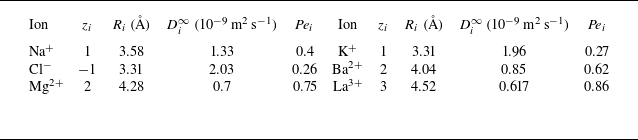


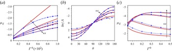


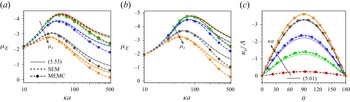


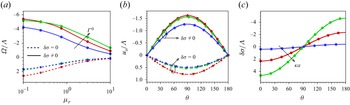


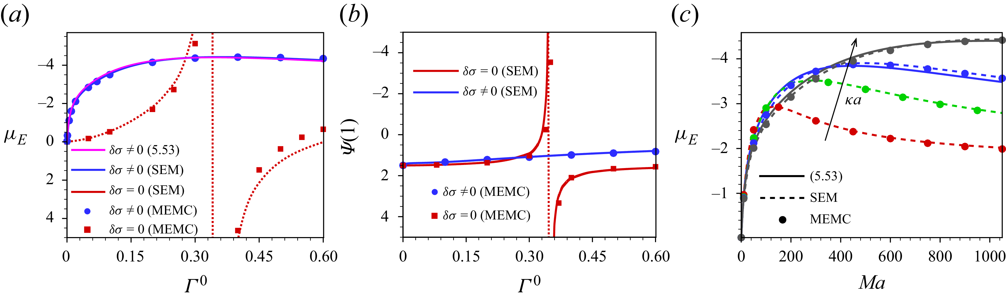


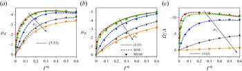


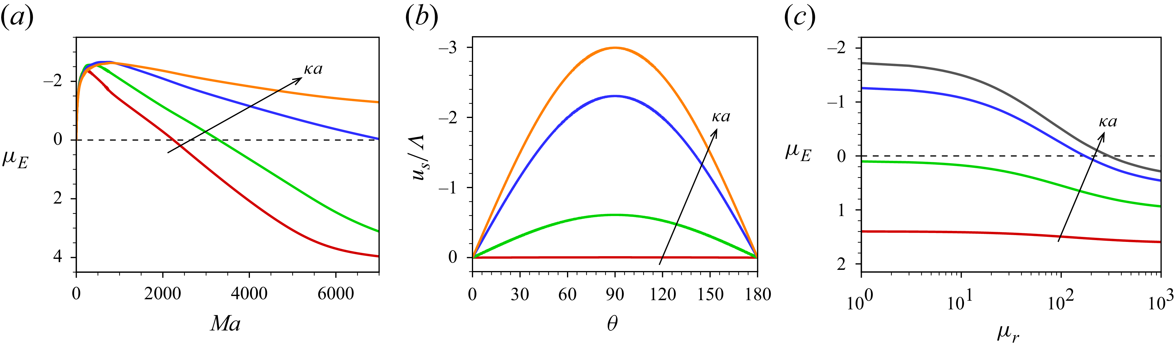


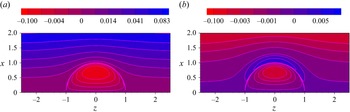


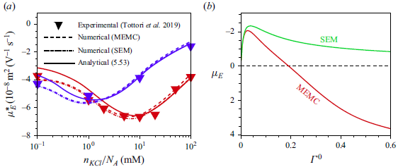


 Open access