


1. Introduction
The formation of wood is pivotal for the development, functioning and adaptation of trees to environmental factors (Cuny et al., Reference Cuny, Rathgeber, Frank, Fonti, Makinen, Prislan and Fournier2015; Rathgeber et al., Reference Rathgeber, Cuny and Fonti2016). In addition, phenology has been demonstrated to be a vital element of tree growth and forest productivity (Albert et al., Reference Albert, Restrepo-Coupe, Smith, Wu, Chavana-Bryant, Prohaska and Saleska2019; Delpierre et al., Reference Delpierre, Berveiller, Granda and Dufrene2016). Furthermore, tree radial growth has been shown to correlate with biomass production and carbon sequestration (Barford et al., Reference Barford, Wofsy, Goulden, Munger, Pyle, Urbanski and Moore2001; Cabon et al., Reference Cabon, Kannenberg, Arain, Babst, Baldocchi, Belmecheri and Anderegg2022). Wood formation is a complex process that occurs beneath the bark of trees and is therefore challenging to observe (Albert et al., Reference Albert, Restrepo-Coupe, Smith, Wu, Chavana-Bryant, Prohaska and Saleska2019). To observe the xylogenesis process directly, it is necessary to take small samples of wood (microcores) and process them in the laboratory for anatomical observation under the microscope (Rossi et al., Reference Rossi, Deslauriers and Anfodillo2006a). A detailed analysis of the obtained anatomical data allows us to accurately describe the wood phenology, i.e. the onset and cessation dates of the different stages of the xylogenesis process (Rathgeber et al., Reference Rathgeber, Longuetaud, Mothe, Cuny and Le Moguédec2011, Reference Rathgeber, Santenoise and Cuny2018).
In the context of climatic changes, numerous studies have investigated the effect of meteorological conditions on the onset, cessation and duration of tree stem growth (e.g. Rossi et al., Reference Rossi, Deslauriers, Anfodillo, Morin, Saracino, Motta and Borghetti2006b, Reference Rossi, Anfodillo, Cufar, Cuny, Deslauriers, Fonti and Rathgeber2013; Huang et al., Reference Huang, Ma, Rossi, Biondi, Deslauriers, Fonti and Ziaco2020). Many of these studies used wood samples (e.g. microcores) for histological observations of wood formation, at the cost of intense field and lab work (Cuny et al., Reference Cuny, Fonti, Rathgeber, von Arx, Peters and Frank2019; Marchand et al., Reference Marchand, Gričar, Zuccarini, Dox, Marien, Verlinden and Campioli2025; Moser et al., Reference Moser, Fonti, Büntgen, Esper, Luterbacher, Franzen and Frank2009). To avoid these costs, many other studies used records of stem radius or girth variations from dendrometers to obtain information on wood growth (e.g. Deslauriers et al., Reference Deslauriers, Rossi and Anfodillo2007; Dow et al., Reference Dow, Kim, D'Orangeville, Gonzalez-Akre, Helcoski, Herrmann and Anderson-Teixeira2022; McMahon et al., Reference McMahon, Parker and Miller2010; Zweifel et al., Reference Zweifel, Sterck, Braun, Buchmann, Eugster, Gessler and Etzold2021). Dendrometers are devices used to measure variations in the size of a tree trunk at more or less regular intervals (Drew & Downes, Reference Drew and Downes2009). There are several types of dendrometers, depending on whether they are automatic or manual, or whether they measure the radius of a tree or its circumference. A number of studies have been conducted in an attempt to ascertain the most effective method of analysing dendrometer readings for the purpose of estimating the beginning and end of tree radial growth (e.g. Cruz-García et al., Reference Cruz-García, Balzano, Čufar, Scharnweber, Smiljanić and Wilmking2019; Korpela et al., Reference Korpela, Mäkinen, Nöjd, Hollmn and Sulkava2010; Miller et al., Reference Miller, Stangler, Larysch, Honer, Seifert and Kahle2022). The majority of these studies concluded that the implementation of logistic growth curves, in conjunction with thresholds of 5 and 95%, represented the optimal approach (e.g. McMahon & Parker, Reference McMahon and Parker2015; Miller et al., Reference Miller, Stangler, Larysch, Honer, Seifert and Kahle2022). This finding is of particular interest as this approach can be applied to all types of dendrometers, provided that the measurement frequency is sufficient (at least monthly).
Comparison of dendrometer records with microcore observations has proved useful in understanding the temporal dynamics of the tree-ring formation process (e.g. Cocozza et al., Reference Cocozza, Palombo, Tognetti, La Porta, Anichini, Giovannelli and Emiliani2016). However, these two approaches have mainly been compared between different trees growing in the same stands with similar growth rates (e.g. Mäkinen et al., Reference Mäkinen, Seo, Nöjd, Schmitt and Jalkanen2008). Only a couple of studies have compared dendrometer records and microcore observations on the same trees, and these studies have not focused on wood phenology (Cuny et al., Reference Cuny, Rathgeber, Lebourgeois, Fortin and Fournier2012; Michelot et al., Reference Michelot, Simard, Rathgeber, Dufrêne and Damesin2012; Ziaco et al., Reference Ziaco, Biondi, Rossi and Deslauriers2016; Güney et al., Reference Güney, Küppers, Rathgeber, Şahin and Zimmermann2017). Therefore, the reliability of dendrometer records in providing estimates of wood phenology has not yet been properly assessed. In order to address this knowledge gap, data were collected from dendrometers and microcores on the same trees, and the critical dates estimated using the dendrometers were then compared with those obtained from the microcores. The dataset under consideration included five tree species, exhibiting contrasting phylogenetic groups (gymnosperms vs. angiosperms), tree-ring structures (i.e. non-porous, diffuse and ring porous), bark types (i.e. smooth, scaled, fissured), site conditions (warm vs. cold) and climatic years (humid vs. dry).
2. Methods
2.1. Datasets and study sites
The present study is based on data coming from three distinct datasets: the ‘Donon’, ‘Mélézin’ and ‘Hesse’ datasets. These three datasets have in common to contain weekly xylogenesis observations and manual band dendrometer data collected on the very same trees.
The “Donon” dataset was produced during the course of Henri Cuny’s PhD thesis (Cuny, Reference Cuny2013a) and has already been used as the basis for several publications (e.g. Cuny et al., Reference Cuny, Rathgeber, Lebourgeois, Fortin and Fournier2012, Reference Cuny, Rathgeber, Frank, Fonti and Fournier2014, Reference Cuny2013b, Reference Cuny, Rathgeber, Frank, Fonti, Makinen, Prislan and Fournier2015, Reference Cuny, Fonti, Rathgeber, von Arx, Peters and Frank2019; Cuny & Rathgeber, Reference Cuny and Rathgeber2016). The dataset includes three sites spread along the slope of the Donon mountain: Walscheid (370 m ASL, 48°38'90''N, 7°099E), Abreschviller (430 m ASL, 48°36'90''N, 7°08'90''E), and Grandfontaine (650 m ASL, 48°28'09'', 7°08'90''E). At each site, three species of conifer: silver fir (Abies alba Mill.), Norway spruce (Picea abies L.), and Scots pine (Pinus sylvestris L.) were growing in mature mixed stands. Based on comprehensive inventories of the stands, five dominant and healthy trees of each species were selected each year for monitoring wood formation. Microcores and dendrometer records were collected on a weekly basis at breast height on the stem of the selected trees from 2007 to 2009, amounting to a total of 135 tree-year series (5 trees x 3 species x 3 plots x 3 years). Daily meteorological data (temperature, precipitation, cumulative global radiation, wind speed and relative humidity) of the period 2007 to 2009 were gathered from three meteorological stations located in the vicinity of the study sites. Over the past three decades, mean annual temperatures were: 8.74, 8.55 and 7.73 °C, while total annual precipitation was: 1159, 1253 and 1532 mm, for Walsheid, Abreschviller and Grandfontaine, respectively. While 2007 and 2009 exhibited lower spring precipitations than the average, 2008 exhibited higher spring precipitations.
The ‘Mélézin’ dataset was produced during Masoumeh Saderi’s PhD thesis (Saderi, Reference Saderi2017) and has been used in two publications (Delpierre et al., Reference Delpierre, Lireux, Hartig, Camarero, Cheaib, Čufar and Rathgeber2019; Saderi et al., Reference Saderi, Rathgeber, Rozenberg and Fournier2019). This dataset includes four instrumented sites spread along an elevation gradient at 1350, 1700, 2000, and 2300 m ASL. The elevation gradient is centred on the Mélézin hamlet (44°51'29''N, 6°38'26''E, 1898 m ASL), which belongs to the municipality of Villard St. Pancrace, located in proximity to the city of Briançon, in the Southern French Alps. Fifteen dominant and healthy European larches (Larix decidua L.) were selected per elevation levels. Microcores and dendrometer records were collected on a weekly basis at breast height on the stem of the selected trees from April to October 2013 for a total of 60 tree-year series (15 trees x 1 species x 3 plots x 1 year). Weather stations were installed along the elevation gradient in small clearings close to the monitored stands to record meteorological data. The daily minimum, maximum, and mean temperatures, along with air humidity, vapor pressure deficit, global radiation and wind speed, were directly obtained from these local weather stations. Daily precipitations from Villard St. Pancrace meteorological station (1300 m a.s.l.) were provided by Météo-France. We combined Villard St. Pancrace daily data and WorldClim 2 (Fick & Hijmans, Reference Fick and Hijmans2017) monthly lapse rates, to compute daily precipitations for the four elevation levels (see Saderi (Reference Saderi2017) for more details).
The ‘Hesse’ dataset was produced during Anjy Andrianantenaina’s (Reference Andrianantenaina2019a) and Ignatius Adikurnia’s PhD theses, and has been partially published in one article (Andrianantenaina et al., Reference Andrianantenaina2019b). This dataset includes one site (48°40’36”N, 7°04’06”E) located in the Hesse forest, which is situated close to the Hesse village, in north-eastern France. This site is a class 1 ecosystem site (FR-Hes) of the Integrated Carbon Observation System (ICOS), which has an Eddy covariance flux tower that measures ecosystem fluxes as well as meteorological and ancillary variables. The studied stand is a young beech forest, interspersed with some oaks. For each year of observation, from 2015 to 2019, seven dominant and healthy European beech (Fagus sylvatica L.) and sessile oak (Quercus petraea (Matt.) Liebl.) trees were selected. Microcores and dendrometer records were collected on a weekly basis at breast height on the stem of the selected trees from March 2015 to October 2019 for a total of 70 tree-year series (7 trees x 2 species x 5 years). Mean annual temperature and mean annual precipitation were 9.5 °C and 885 mm, respectively, over the last 30 years. All study years were characterised by higher-than-average temperatures, with 2015 and 2018 being drier than average and 2016, 2017 and 2019 being wetter than average, particularly during the spring months.
2.2. Tree species life traits and individual characteristics
The final dataset comprises six tree species characterised by contrasting life traits (Supplementary Table S1). Among the species under consideration, there are four gymnosperm species (silver fir, Scots pine, Norway spruce and European larch) and two angiosperm species (European beech and sessile oak). Silver fir and Norway spruce present homogeneous non-porous growth rings (encompassing transition wood in between early- and late-wood) and quite thick scaly bark, while European larch and Scots pine present heterogenous non-porous growth rings (exhibiting an abrupt transition between early- and late-wood) and thick fissured bark (see Cuny et al., Reference Cuny, Rathgeber, Frank, Fonti and Fournier2014, for more details about the tree-ring structure). European beech presents diffuse porous growth rings and a thin, smooth bark, while sessile oak presents ring-porous growth rings and very thick fissured bark.
The characteristics of the studied tree populations were also contrasted. The beech and oak trees, which were growing in a young stand, were the thinnest (diameter at breast height (DBH) of 25.2 ± 2.4 and 26.1 ± 2.9 cm, respectively), the smallest (height of 19.5 ± 4.8 and 19.8 ± 4.2 m, respectively) and the youngest (age of 55 ± 3.6 and 40.6 ± 1.5 years, respectively). Larch trees, which were growing in mature to old stands, were intermediate in terms of dimensions (DBH of 44.2 ± 7.5 cm and height of 23.3 ± 4.9 m) despite being the oldest (age of 155.9 ± 39.2 years) (Supplementary Table S2). Finally, Fir, spruce and pine trees, which were growing in mature stands, were the thickest (DBH of 58.5 ± 6.0, 50.2 ± 8.7 and 56.3 ± 7.3 cm, respectively), tallest (height of 32.9 ± 3.3, 32.3 ± 1.9 and 31.5 ± 4.4 m, respectively) and quite old (age of 101 ± 26.7, 82.8 ± 12.2 and 125.2 ± 29.4 years, respectively).
2.3. Wood microcore approach
For one to three growing seasons, microcores (i.e. wood samples of 2 mm in diameter and 15-20 mm in length) were taken weekly from the stem at breast height of all selected trees using a Trephor® tool (Vitzani, Belluno, Italy) following an ascending spiral pattern (Rossi et al., Reference Rossi, Deslauriers and Anfodillo2006a). Immediately after extraction, the microcores were placed in a solution of 50% ethanol and then stored at 5°C before being dehydrated in the laboratory by successive immersions in baths of ethanol and d-limonene and embedded in paraffin according to classical protocols (Rossi et al., Reference Rossi, Deslauriers and Anfodillo2006a). Transverse sections, 5-10 μm thick, were cut on a rotary microtome, stained with cresyl violet acetate or safranin and astra blue, and permanently mounted on glass slides (Fonti et al., Reference Fonti, von Arx, Harroue, Schneider, Nievergelt, Björklund and Fonti2025). In total, more than 8,000 anatomical sections were observed under white and polarised lights at 125–400 magnifications, using an optical microscope to describe the temporal changes in forming xylem over the monitored growing seasons.
In xylogenesis studies, the formation of a xylem cell is commonly categorised into four distinct differentiation phases: (i) the dividing phase, during which the division of a cambial mother cell gives rise to a new daughter cell; (ii) the enlarging phase, during which the newly formed xylem cell undergoes radial expansion; (iii) the thickening phase, characterised by the formation of secondary walls and the lignification of cell walls; and finally (iv) the programmed cell death, which marks the conclusion of cell differentiation and the advent of mature, fully functional tracheary element (Rathgeber et al., Reference Rathgeber, Cuny and Fonti2016).
The sorting of cells in the cambial, cell-enlarging, wall-thickening and mature zones was conducted in accordance with the criteria established by Rossi et al. (Reference Rossi, Deslauriers and Anfodillo2006a). In cross-section, cambial cells were distinguished by their thin cell walls and diminutive radial diameters. In contrast, cells in the enlargement phase exhibited radial diameters at least twice as larger as cambial cells and possessed thin walls. Cells in the wall thickening and lignification phase exhibited birefringence under polarised light, while displaying bi-coloured walls. Xylem cells were considered mature when their walls were completely stained in a single, uniform colour (blue with cresyl violet acetate or red with safranin and astra blue).
For the gymnosperm species, the number of cells in the cambial, cell-enlarging, wall-thickening and mature zone, along with the number of cells in the previous ring (i.e. the tree-ring formed during the previous growing season), were counted along at least three radial files, according to the criteria described above (see Cuny et al., Reference Cuny, Rathgeber, Lebourgeois, Fortin and Fournier2012 for more details). For the angiosperm species, the width of the cambial, cell-enlarging, wall-thickening and mature zone for fibre cells, along with the width of the previous ring, were measured in at least three different regions of the section (see Dox et al. (Reference Dox, Prislan, Gričar, Marien, Delpierre, Flores and Campioli2021) for more details). The final xylogenesis dataset comprises approximately 100,000 cell counts or width measurements, constituting the elementary raw data.
The present study focuses on the onset and cessation of the period of xylem cell enlargement, which also demarcates the beginning and end of stem wood growth (Rathgeber et al., Reference Rathgeber, Cuny and Fonti2016). At the beginning of the growing season, the onset of xylem cell enlargement (b E) is defined as the date at which 50% of the observed radial files for gymnosperm, or section regions for angiosperm species, present at least one first enlarging cell. The cessation of xylem cell enlargement (c E) is defined as the date at which 50% of the observed radial files for gymnosperms, or section regions for angiosperms, present at most one last enlarging cell. The estimation of b E and c E was made using the ‘computeCriticalDates’ function of the R-package CAVIAR (Rathgeber et al., Reference Rathgeber, Longuetaud, Mothe, Cuny and Le Moguédec2011), which employs logistic regressions to analyse the counts of enlarging cells (for gymnosperms) or the widths of enlarging bands (for angiosperms).
2.4. Manual band dendrometer approach
A few weeks prior to the commencement of the wood formation monitoring, manual band dendrometers (EMS DB20) were installed on all the trees under study. These dendrometers were placed at breast height, after the bark had been cleaned, and above the area where the microcores were to be taken. They were subsequently read with an accuracy of 0.1 mm on a weekly basis, concurrently with the collection of the microcores. The stem girth measurements were then converted into DBH estimates.
The DBH estimates were fitted using a classical five-parameter logistic model approach using the R package RDendrom (McMahon & Parker, Reference McMahon and Parker2015). The observed DBH on a given day of the year (DOY) is modelled as follows:
 $$\begin{align}{\mathrm{DBH}}_{\mathrm{DOY}}=\frac{L+\left(K-L\right)}{1+1/\theta \times \exp {\left[-\mathrm{r}\left(\mathrm{DOY}-{\mathrm{DOY}}_{\mathrm{ip}}\right)/\theta \right]}^{\theta }}\end{align}$$
where L and K are the lower and upper asymptotes of the curve, DOYip is the date of the inflection point, r shapes the slope at the inflection point, and $\theta$
is a tuning parameter controlling the slope towards the upper asymptote. The RDendrom functions take the time series of the dendrometer records and return maximum likelihood-optimized values of the above five parameters that best predict DBH increase over time.
$\theta$
is a tuning parameter controlling the slope towards the upper asymptote. The RDendrom functions take the time series of the dendrometer records and return maximum likelihood-optimized values of the above five parameters that best predict DBH increase over time.
The root mean squared error (RMSE), which measures the difference between the estimated and actual data (Chai & Draxler, Reference Chai and Draxler2014) is used to evaluate the fit of the five-parameter logistic curves. The RMSE is computed as follows:
 $$\begin{align}\mathrm{RMSE}=\sqrt{\frac{\sum_{i=1}^N{\left({\mathrm{DBH}}_i-{\widehat{\mathrm{DBH}}}_i\right)}^2}{N}}\end{align}$$
where ${\mathrm{DBH}}_i$
is the observed stem diameter,
${\mathrm{DBH}}_i$
is the observed stem diameter, $\widehat{{\mathrm{DBH}}_i}$
is the predicted stem diameter (provided by the five-parameters logistic model) and
$\widehat{{\mathrm{DBH}}_i}$
is the predicted stem diameter (provided by the five-parameters logistic model) and $N$
is the number of data points. The RMSE can only take positive values. If the RMSE is equal to zero, this indicates a perfect fit to the data. Therefore, as the RMSE increases, the goodness-of-fit decreases.
$N$
is the number of data points. The RMSE can only take positive values. If the RMSE is equal to zero, this indicates a perfect fit to the data. Therefore, as the RMSE increases, the goodness-of-fit decreases.
The RDendrom package was then used to calculate the dates on which 5% (DOY.05) and 95% (DOY.95) of the simulated annual growth was completed, based on the parameters of the logistic models previously fitted (McMahon & Parker, Reference McMahon and Parker2015). These dates were used as surrogates for the beginning and the end of stem radial growth.
2.5. Statistical analyses
This study aimed to compare the critical dates obtained using the dendrometer approach (i.e. DOY.05 and DOY.95, the beginning and the end of stem radial growth) with the corresponding critical dates provided by the microcore approach (i.e. b E and c E, the onset and cessation of xylem cell enlargement). The dispersion of the critical dates produced by the dendrometer and the microcore approaches was calculated using classical measures of variance (e.g. standard deviation) as well as visualisation tools (e.g. boxplots). The difference between the values produced by the two approaches was calculated, at the elementary level, as the absolute difference (AD, in days) between dendrometer and microcore dates. Moreover, at the group level, mean absolute difference (MAD, in days) and root mean square difference (RMSD, in days) were used to assess the differences between dendrometer and microcore dates. Note that RMSD and RMSE share the same mathematical formula, but for clarity, we speak about RMSE when assessing the level of error of a model and about RMSD when assessing the level of difference between two estimates. AD, MAD were computed as follows:
 $$\begin{align}{\mathrm{AD}}_i=\left|{\mathrm{microCD}}_i-{\mathrm{dendroCD}}_i\right|\end{align}$$
 $$\begin{align}\mathrm{MAD}=\frac{\sum_{i=1}^N\left|{\mathrm{microCD}}_i-{\mathrm{dendroCD}}_i\right|}{N}\end{align}$$
where ${\mathrm{microCD}}_i$
is the critical date provided by the microcore approach,
${\mathrm{microCD}}_i$
is the critical date provided by the microcore approach, ${\mathrm{dendroCD}}_i$
is critical date provided by the dendrometer approach, and
${\mathrm{dendroCD}}_i$
is critical date provided by the dendrometer approach, and $N$
is the number of data points.
$N$
is the number of data points.
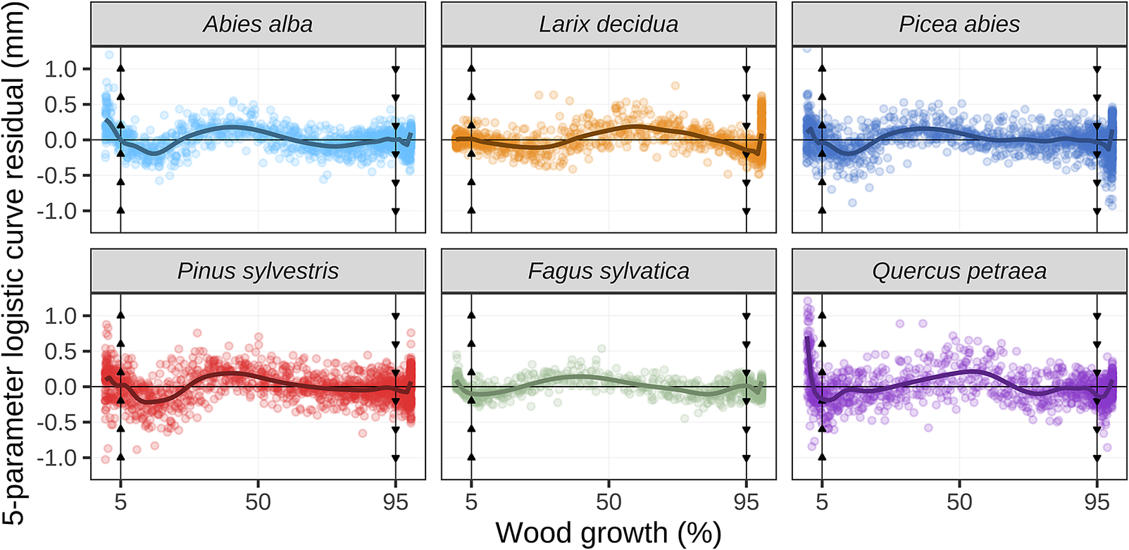
Figure 1. Plots of the residuals of the five-parameter logistic growth model applied to dendrometer measurements. Data points represent the residuals. The x-axis is presented in percentage of the annual growth (rather than day of year) to facilitate comparison of data from different trees, sites and years. The vertical arrowed lines mark the 5% and 95% growth thresholds. The solid lines represent the generalized additive models fitted to the residuals to highlight the overall patterns.
Following Rossi et al. (Reference Rossi, Anfodillo, Cufar, Cuny, Deslauriers, Fonti and Rathgeber2013), we performed reduced major axis (RMA) regression to assess any bias in the dendrometer approach. RMA regression minimises the sum of the product of both vertical and horizontal deviations, which is equivalent to the area of the triangles formed by the deviation of a point from the line in the vertical and horizontal directions (Smith, Reference Smith2009). RMA regression was more appropriate than the conventional ordinary least squares regression because here both response variables (DOY.05 and DOY.95) and predictors (b E and c E) were estimated with errors (Mesplé et al., Reference Mesplé, Troussellier, Casellas and Legendre1996). Thereafter, the 95% confidence interval was employed to test the null hypothesis that the intercept was not significantly different from zero and that the slope was not significantly different from one. This was done to check for an offset (i.e. whether the confidence interval around the intercept does not include zero) and/or a bias (i.e. whether the confidence interval around the slope does not include 1) in the dendrometer estimates.
Finally, the T-test and ANOVA were performed to evaluate the differences between different groups of species and growing conditions. All data were prepared and analysed using the programming language R version 4.1.0 (R Core Team, 2022).
3. Results
3.1. Goodness of fit of the logistic growth models
Overall, the dendrometer records showed S-shaped growth patterns that were well fitted by the five-parameter logistic growth model with a combined average RMSE of 0.17 ± 0.06 mm. Nevertheless, important differences in the goodness of fit were observed between species. The European beeches exhibited the best fittings, followed by the firs, larches, spruces, pines, and oaks (RMSE = 0.10, 0.16, 0.18, 0.20, 0.21 and 0.24 mm, respectively; Supplementary Figures S3–S8).
An analysis of the residuals showed that the quality of the fittings varied throughout the growing period (Figure 1). For the 5% growth threshold, the fittings were accurate for the gymnosperms (firs, larches, pines and spruces), but not for the angiosperms (beeches and oaks). For the 95% growth threshold, the fittings were accurate for the beeches, firs, pines and spruces, but not for the larches and oaks. Indeed, the firs, spruces, pines and oaks commonly exhibited stem shrinkage at the beginning of the vegetation season, while larches kept increasing stem diameter until the end of the year (Supplementary Figure S9).
3.2. Comparison between dendrometer and microcore estimates of wood phenology
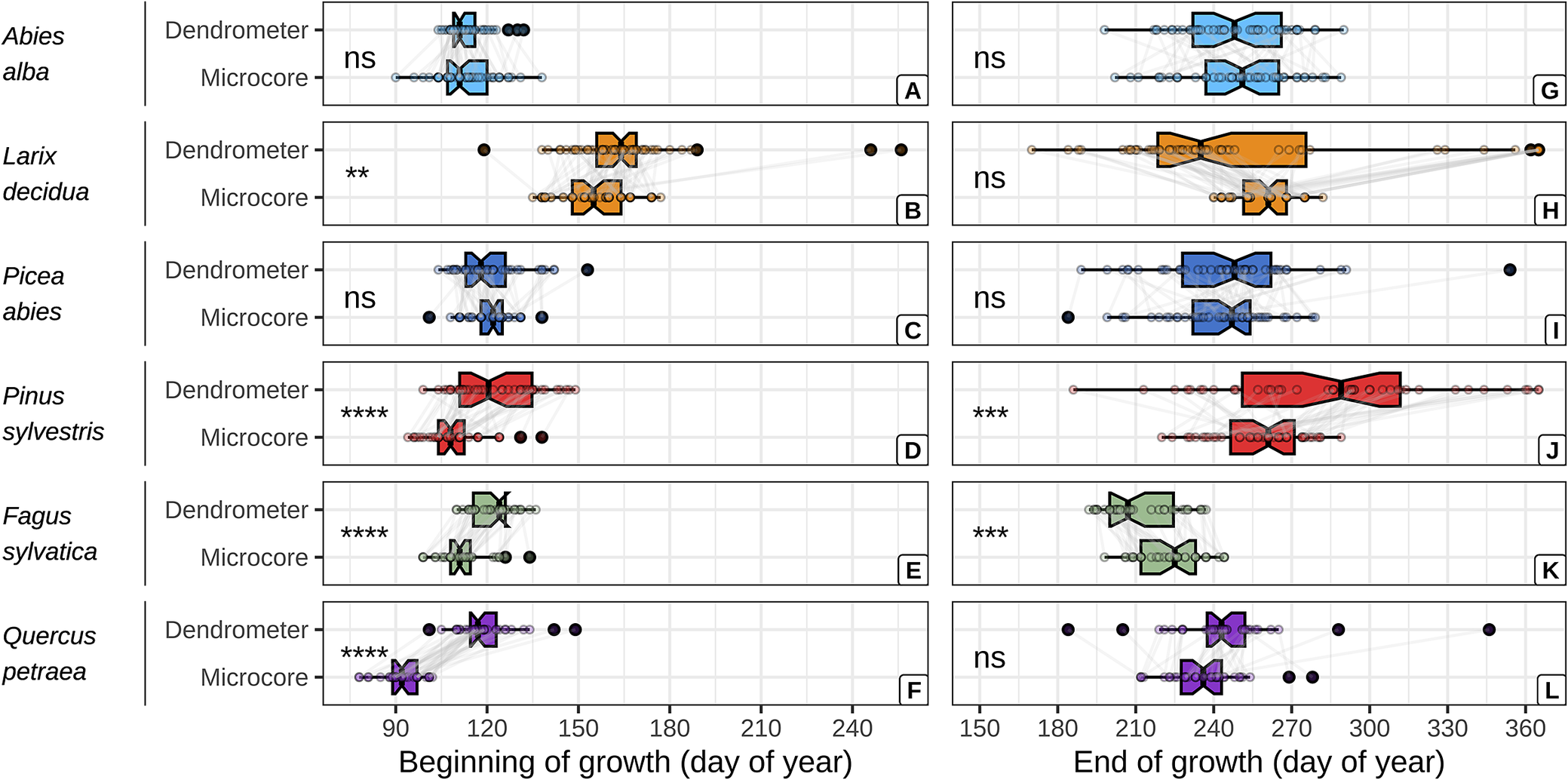
The dendrometer and microcore approaches yielded comparable estimates of the beginning and end of wood growth for firs and spruces (Figure 2, Supplementary Table S10). However, the dendrometer approach yielded systematically later estimates of the beginning of wood growth for the other species. With mean absolute difference (MAD) increasing from the larches, beeches, pines and oaks (MAD = 9 ± 24, 10 ± 6, 13 ± 13 and 27 ± 11 days, respectively). Moreover, the dendrometer approach yielded earlier estimates of the end of wood growth for the larches and beeches (MAD = 0 ± 62 and 12 ± 10 days, respectively) and later ones for the oaks and pines (MAD = 8 ± 23 and 28 ± 48 days, respectively).

Figure 2. Comparison between dendrometer and microcore estimates of the beginning and the end of wood growth, for each studied species. The critical dates derived from both approaches for a given tree are represented by points connected with grey lines. The significance of the mean comparison test (t-test) is indicated on the left side of each plot and is denoted as follows: * for p < 0.05, ** for p < 0.01, *** for p < 0.001, **** for p < 0.0001, and ns for p ≥ 0.05.
Further investigation using reduced major axis (RMA) regressions of the relationship between dendrometer- and microcore-based estimates showed that the dendrometer approach provided better estimates of the beginning of the season than the end in all conifer species (Figure 3, Supplementary Table S11). Among the six studied species, only the beeches and firs presented significant relationships for both the beginning and the end of the growing season (p < 0.05). However, even for these two species, the RMA regression analysis showed that the linear relationships between dendrometer and microcore-based estimates presented offsets and bias. The RMA regression analysis further revealed the presence of biased linear relationships for the pines and the spruces at the beginning of the growing season. Moreover, for the pines, the spruces and the larches, the analysis also showed the absence of relationships between dendrometer and microcore-based estimates at the end of the growing season. For these three species, microcores estimates presented a variability of approximately one month, while dendrometer estimates exhibited a surprisingly high variability of approximately six months. Finally, for oaks, the relationship was not significant at the beginning of the growing season, but it was significant at the end (p < 0.05).
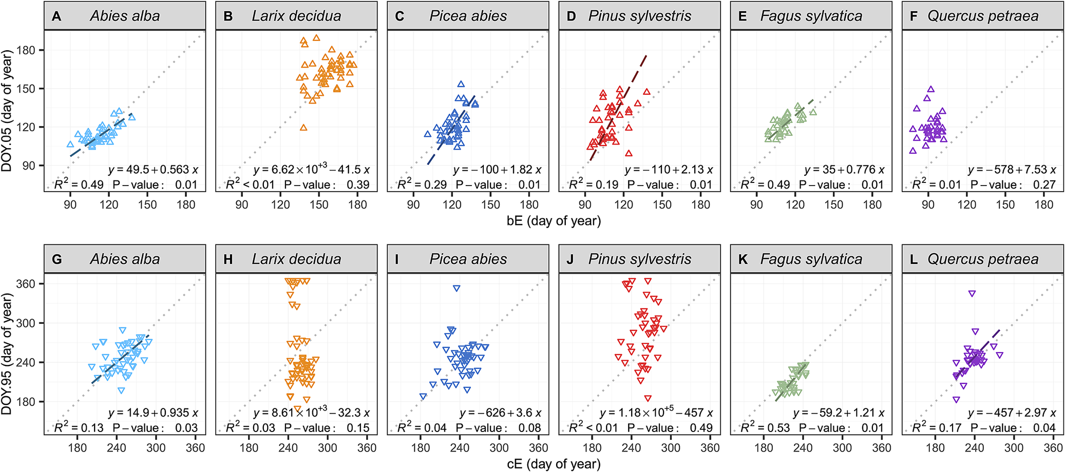
Figure 3. Relationships between dendrometer and microcore estimates of the beginning and the end of wood growth (DOY.05 and DOY.95 and b E and c E, respectively), for each studied species. The data points represent single-year values for each tree. The dotted lines represent the x:y baseline, while the striped lines represent the significantly reduced major axis (RMA) regressions. The equations of the RMA regressions, the coefficients of determination (R 2), and the p-value of the permutation test are provided in the plots.
3.3. Relationships between life traits and accuracy of dendrometer estimates
Negative significant relationships were found between dendrometer- and microcore-based estimates discrepancies and stem growth rates for the beginning of the growing season for the larches, oaks and pines and for the end of the growing season for the beeches, firs, larches, oaks and pines (Supplementary Figure S12). This suggests that faster growth rates are generally associated with greater accuracy in dendrometer estimates, especially at the end of the growing season. Surprisingly, no significant relationships were found between the goodness-of-fit of the logistic growth models and the discrepancies between dendrometer and microcore-based estimates (Supplementary Figure S13).
While exploring the causes of discrepancy between dendrometers- and microcores-based estimates we found that MAD was significantly greater for angiosperms at the beginning of the growing season and significantly lower at the end (Figure 4a–e). A more detailed analysis of the composition of each taxonomic group revealed that, at the beginning of the growing season, MAD increased with increasing tree-ring structure heterogeneity from homogeneous non-porous and diffuse-porous tree-rings to heterogeneous non-porous and ring-porous ones (Figure 4b). At the end of the growing season, diffuse-porous, ring-porous and homogeneous non-porous tree-rings showed substantial MAD, while heterogeneous non-porous tree-rings showed significantly greater MAD (Figure 4b).
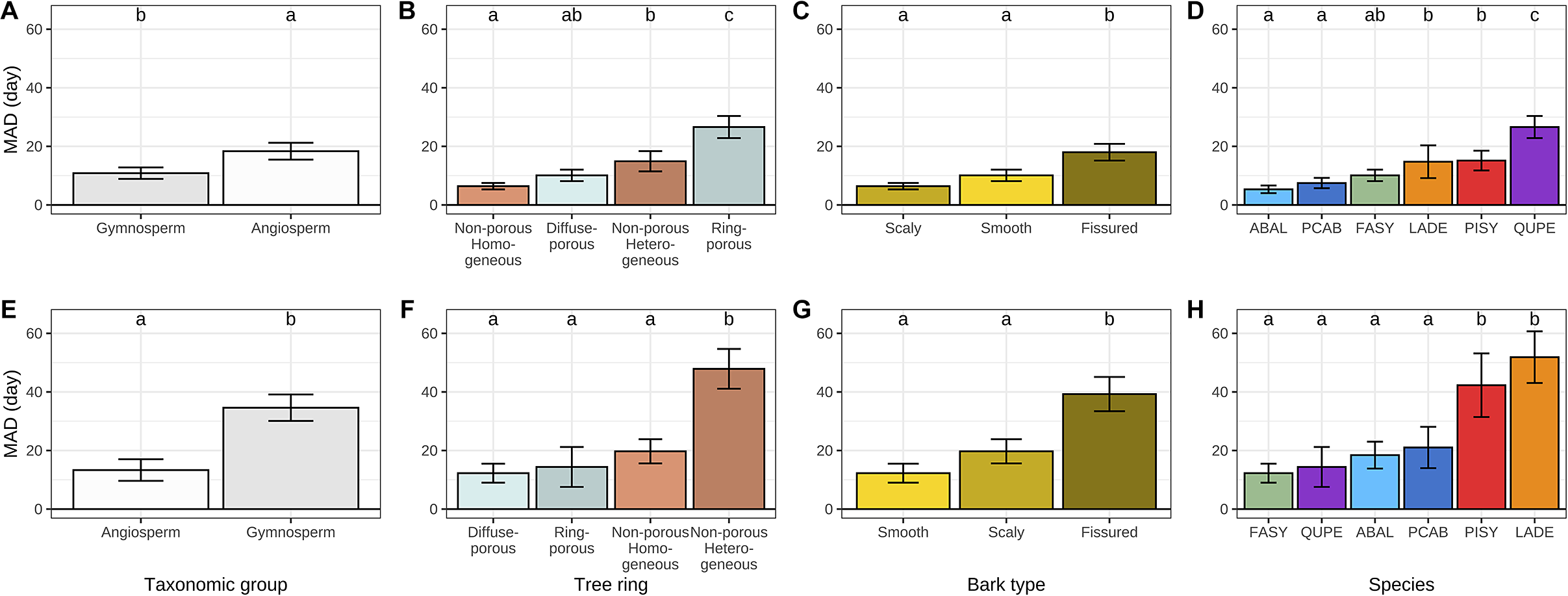
Figure 4. Mean absolute difference (MAD) between dendrometer and microcore-based estimates of the beginning (a–d) and the end (e–h) of wood growth over different life traits, including taxonomic groups, tree-ring structure, bark types and tree species. The whiskers are defined as the 5 and 95 percentiles. The results of the post-hoc Tukey ANOVA test are indicated by small letters above each bar, with shared letters signifying non-statistically different means. In plots D and H, the acronyms ABAL, FASY, LADE, PCAB, PISY and QUPE correspond to the species Abies alba, Fagus sylvatica, Larix decidua, Picea abies, Pinus sylvestris and Quercus petraea, respectively.
The influence of bark traits on discrepancies between dendrometer and microcore-based estimates was also examined. With regard to the beginning of the growing season, the scaly and smooth bark types showed substantial MAD, while the fissured bark type showed significantly greater MAD (Figure 4c). At the end of the growing season, all bark types exhibited much higher MAD than they did at the beginning. However, the overall pattern remained consistent, with only the fissured bark type demonstrating a significantly higher MAD than the smooth and scaly types (Figure 4g). We also investigated the relationships between the accuracy of dendrometer-based estimates and the bark thickness, but we did not find any significant relationship.
A species-level analysis yielded three clusters at the beginning of the growing season and two clusters at its end. With regard to the beginning of the growing season, MAD increased sequentially from the firs, spruces and beeches to the larches and pines, ultimately reaching a peak with the oaks. Concerning the end of the growing season, MAD increased sequentially from the beeches, oaks, firs and spruces to culminate with the pines and larches.
3.4. Relationships between environmental factors and accuracy of dendrometer estimates
In exploring the environmental causes of discrepancies between dendrometer and microcore-based estimates, we found that, at the beginning of the growing season, MAD were greater when springs were wetter. This effect holds at the species level for the firs, beeches and oaks, only the pines and spruces did not present any significant differences (Figure 5a–e, Supplementary Figure S14A). We didn’t observe the same relationships at the end of the growing season, MAD weren’t significantly greater when autumns were wetter (Figure 5g–k, Supplementary Figure S14B).
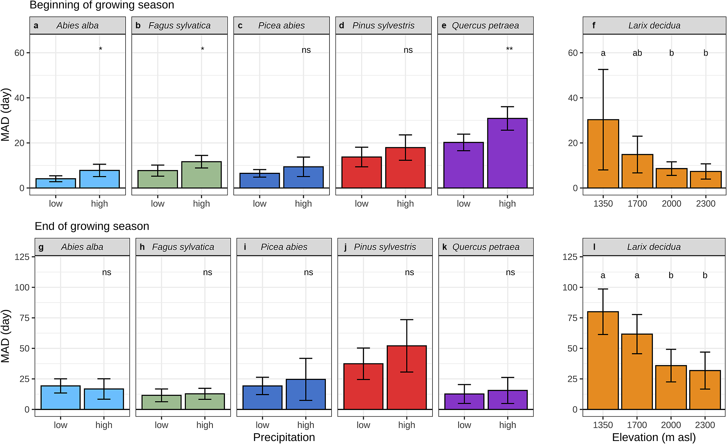
Figure 5. Mean absolute difference (MAD) between dendrometers and microcores at the beginning (a–f) and end (g–l) of wood growth. (a) to (e) illustrate the comparison between two levels of spring precipitation, while (g) to (k) show the comparison for summer precipitation. For (a), (c) and (d), the precipitation data were taken in March and a threshold of 50 mm was used to separate high and low values. In (b) and (e), the precipitation data are measured in April and a threshold of 100 mm is applied. For (g), (i) and (j), the precipitation data are the sum of June, July and August, with a threshold of 300 mm used to separate high and low values. In (h) and (k), the precipitation data are the sum of August, September and October and a threshold of 100 mm is applied (see Supplementary Figure S14 for more details). (f) and (l) show the comparison for four elevation levels. In the lower panel, the whiskers are defined as the 5 and 95 percentiles. For (a) to (e) and (g) to (k) the significance of the mean comparison test (t-test) is indicated on the top of each plot and is denoted as follows: * for p < 0.05, ** for p < 0.01, *** for p < 0.001, **** for p < 0.0001, and ns for p ≥ 0.05. For (f) and (l) the results of the post-hoc Tukey ANOVA tests are indicated by small letters above each elevation, with shared letters signifying non-statistically different means.
We also found a strong effect of elevation on the accuracy of the dendrometer-based estimates. For the larches, at the beginning and the end of the growing season, MAD decreased significantly from the lowest to the highest elevation level (Figure 5f, l). Estimates based on dendrometers lagged behind those based on microcores for the three lowest sites, whereas they were ahead for the highest one.
4. Discussion
4.1. Dendrometer are poor indicators of wood phenology
Manual band dendrometers are inexpensive and easy to use, and they do not harm the trees. This enabled us to place them systematically on all the trees we cored. We always sampled the trees in the same order, even between sites, ensuring that the dendrometers were read at roughly the same time each day and avoiding most diel variation. Therefore, we believe that our manual band dendrometers provided precise measurements of weekly stem girth variations.
A direct comparison of the dendrometer and microcore-based critical dates revealed no statistically significant differences for two species (out of six) regarding the beginning of wood growth, and for four species concerning the end. However, these favourable outcomes can be attributed to the substantial variability observed in critical dates, particularly towards the end of the growing season and do not imply a strong agreement between the two approaches. Indeed, a deeper investigation into the relationships between the dendrometer and microcore-based estimates revealed the absence of a relationship for two species concerning the beginning of wood growth and for three species regarding the end. Furthermore, in instances where a significant relationship was found, it was generally biased or offset.
As is usually the case (e.g. Deslauriers et al., Reference Deslauriers, Rossi and Anfodillo2007; Dow et al., Reference Dow, Kim, D'Orangeville, Gonzalez-Akre, Helcoski, Herrmann and Anderson-Teixeira2022; McMahon & Parker, Reference McMahon and Parker2015), fitting the dendrometer data using the five-parameter logistic model provided excellent results in our study. However, the variability of the critical dates estimated using the dendrometer approach is much higher than that obtained using the microcore approach, particularly at the end of wood growth. This suggests that the inability of the dendrometer-based approach to provide reliable critical dates is not due to the accuracy of the dendrometers or the quality of the growth model adjustments, but rather to the use of thresholds (5% and 95% in our case) for extracting critical dates from the curves generated by these models. Logistic growth curves and assimilated methods (e.g. Deslauriers et al., Reference Deslauriers, Rossi and Anfodillo2007) are highly effective in modelling the annual dynamics of wood growth, particularly during the core of the season (e.g. Dow et al., Reference Dow, Kim, D'Orangeville, Gonzalez-Akre, Helcoski, Herrmann and Anderson-Teixeira2022). However, they are not well defined at the boundaries of the growing season, when growth rates are low and the overall growth contribution is negligible.
Automatic point dendrometers could have been used instead of manual band dendrometers. The main advantages are greater precision and the ability to provide sub-hourly measurements of stem radius variations. This allows diel variations to be taken into account properly, rather than trying to exclude them (De Swaef et al., Reference De Swaef, De Schepper, Vandegehuchte and Steppe2015). However, as well as being harmful to trees, they only provide information for one point around the tree circumference. Consequently, we found them to be less suitable for comparison with microcores, which also only provide anatomical information at a single point around the circumference. For a given tree, the microcore sampling point changes every week, whereas the dendrometer stays in the same place. This could introduce a significant random component to the comparison of the two approaches, as growth variability could be high around the stem.
The zero-growth approach (Zweifel et al., Reference Zweifel, Haeni, Buchmann and Eugster2016) has produced excellent results in describing and relating growth patterns to climate conditions over a year (e.g. Bose et al., Reference Bose, Etzold, Meusburger, Gessler, Baltensweiler, Braun and Zweifel2025; Etzold et al., Reference Etzold, Sterck, Bose, Braun, Buchmann, Eugster and Zweifel2021). However, based on our reasoning, the method may not be useful for assessing wood phenology, since critical dates would also be computed by applying thresholds to cumulative curves (Jankowski et al., Reference Jankowski, Calama, Aldea, García, Madrigal and Pardos2025). Building on the pioneering work of King et al. (Reference King, Fonti, Nievergelt, Büntgen and Frank2013) and Cocozza et al. (Reference Cocozza, Palombo, Tognetti, La Porta, Anichini, Giovannelli and Emiliani2016), a promising approach to estimating critical dates of wood phenology using automatic point dendrometers would be to analyse the diel cycles of diameter variations, rather than the growth signal itself, in order to characterise the state of the forming xylem (e.g. cambium at rest, growing new xylem or maturing new xylem).
4.2. Contribution of phloem and bark to stem girth variations
Despite the frequent use of dendrometers to estimate wood phenology (e.g. Bose et al., Reference Bose, Etzold, Meusburger, Gessler, Baltensweiler, Braun and Zweifel2025; Deslauriers et al., Reference Deslauriers, Rossi and Anfodillo2007; Dow et al., Reference Dow, Kim, D'Orangeville, Gonzalez-Akre, Helcoski, Herrmann and Anderson-Teixeira2022; van der Maaten et al., Reference van der Maaten, Pape, van der Maaten-Theunissen, Scharnweber, Smiljanic, Cruz-Garcia and Wilmking2018), it is important to note that these instruments record the growth signals of both the xylem and the phloem (Mencuccini et al., Reference Mencuccini, Salmon, Mitchell, Hölttä, Choat, Meir and Pfautsch2017). Moreover, as well as recording the growth of living tissue, dendrometers also pick up signals related to the moisture content of living and dead tissue (xylem, phloem and periderm), as well as signals related to tissue and device temperature (De Swaef et al., Reference De Swaef, De Schepper, Vandegehuchte and Steppe2015).
Current knowledge suggests that early phloem cell differentiation occurs slightly before that of early xylem cells. This ensures that the tree can transport sugars from the leaves to fuel cambial activity. This timing difference is most pronounced in ring-porous species and less so in diffuse-porous species; it is also present in non-porous species (Evert, Reference Evert2006; Gričar, Reference Gričar2024). However, our results on six different tree species (beech, fir, larch, pine, oak and spruce) in temperate and mountain forests confirm previous works on Norway spruce in boreal forests (Mäkinen et al., Reference Mäkinen, Seo, Nöjd, Schmitt and Jalkanen2008) and on Scots pine, European beech, and sessile oak in temperate forests (Michelot et al., Reference Michelot, Simard, Rathgeber, Dufrêne and Damesin2012) indicating later dates for dendrometer estimates than for microcores. Moreover, the response of xylem and phloem to external stimuli is not necessarily coordinated, as has been shown in the case of heating and cooling experiments in Norway spruce (Gričar et al., Reference Gričar, Zupančič, Čufar, Koch, Schmitt and Oven2006) or in post-fire response in pubescens oak stems (Gričar et al., Reference Gričar, Hafner, Lavric, Ferlan, Ogrinc, Krajnc and Vodnik2020). In both cases, the phloem was the first to respond to the increased temperature.
Dendrometers also integrate signal from the periderm and especially its water content (De Swaef et al., Reference De Swaef, De Schepper, Vandegehuchte and Steppe2015). Indeed, in Spring, a dehydration–rehydration cycle (a particularly salient phenomenon in angiosperm species in relation to the process of leaf unfolding) frequently coincides with the onset of xylem formation (Shtein et al., Reference Shtein, Gričar, Lev-Yadun, Oskolski, Pace, Rosell and Crivellaro2023), thereby obscuring the xylem growth signal in dendrometer data. In a similar manner, the progressive rehydration of the bark in Autumn, following the summer dehydration period, can mask the discrete cessation of xylem growth (van der Maaten et al., Reference van der Maaten, Pape, van der Maaten-Theunissen, Scharnweber, Smiljanic, Cruz-Garcia and Wilmking2018). General Additive Models (GAM) could provide an efficient means to fit dendrometer recordings more closely and take into account the seasonal dehydration–rehydration cycle (Cuny, Reference Cuny2013b). However, this would not necessarily improve critical dates estimation (Miller et al., Reference Miller, Stangler, Larysch, Honer, Seifert and Kahle2022).
4.3. Influences of life traits on dendrometer estimate accuracy
The species under scrutiny exhibited contrasting sets of relationships between the dendrometers and microcore-based critical dates. At the beginning of the growing season, the dendrometer approach overestimated the start of wood production for four species (pine, larch, beech and oak) while two species demonstrated no significant differences (fir and spruce). These results were largely explained by the bark types. Indeed, smooth and scaly barks (beech, fir and spruce) are relatively thin, while fissured barks (pine, larch and oak) are thick and undergo substantial cycles of shrinkage and swelling (Shtein et al., Reference Shtein, Gričar, Lev-Yadun, Oskolski, Pace, Rosell and Crivellaro2023). The observation that even ring-porous oak, which initiates xylem formation with a distinctive surge of growth to produce its substantial early wood vessels, is not detected by dendrometers at the beginning of wood growth underscores the major contribution of bark in spring stem girth variations.
At the end of the growing season, the variability in dendrometer estimates was such that it prevented us from finding significant differences in four species (fir, pine, larch and oak).
However, a slight tendency for dendrometers to overestimate the end of wood formation (i.e. estimate it later) for fissured bark (e.g. pine) while underestimating it (i.e. estimate it earlier) for scaly and smooth barks (e.g. beech) was observed. Although the rehydration of bark during the autumn may provide a rationale for the overestimation observed in fissured barks, the underestimation seen in smooth barks remains to be explained.
4.4. Influences of environmental factors on dendrometer estimate accuracy
In exploring the influences of environmental factors, we found that the discrepancies between dendrometer- and microcore-based estimates of wood phenology were greater when springs were wetter. Furthermore, contrary to what we expected from Tumajer et al. (Reference Tumajer, Scharnweber, Smiljanic and Wilmking2022), no discernible effect of vapour pressure deficit was observed on the accuracy of dendrometer-based estimates. Although these results are difficult to interpret in terms of ecophysiological mechanisms, they clearly demonstrate that changes in the water balance alter the accuracy of dendrometer-based estimates.
We also found a strong effect of temperature on the accuracy of dendrometer-based estimates. For larch, the discrepancies between dendrometer and microcore increased from the highest to the lowest site along a 1,000 m elevation gradient – representing a 5°C transect in mean annual temperature. These results show that the dendrometer approach can yield good estimates of wood phenology in very cold sites, but its accuracy drops as the temperatures rise.
5. Conclusion
Our study exposes the complexities of using dendrometers to assess wood phenology critical dates. We have shown that dendrometer measurements provide biased estimates of the beginning, the end and therefore the duration of wood growth. The discrepancies between dendrometer- and microcores-based estimates can be partially explained by tree species life traits, such as tree-ring structure and bark type. Therefore, we recommend taking these factors into account in future studies. However, we also demonstrated that the discrepancies between dendrometer- and microcores-based estimates are also related to site conditions and climate variations. This complicates the use of dendrometers to study spatial and temporal changes in wood phenology and calls into question the results of this approach regarding the impact of climate change on forest productivity and carbon sequestration. Finally, we argue that dendrometers, which have the capacity to be deployed over large areas and for long periods, should be used in conjunction with microcore-based wood formation monitoring studies. This combination is proposed as a means of compensating for some of the biases of dendrometers and thus enabling their potential to be exploited to the full.
Open peer review
To view the open peer review materials for this article, please visit http://doi.org/10.1017/qpb.2025.10031.
Acknowledgements
The authors would like to thank H. Cuny, M. Saderi and A. Andrianantenaina for providing wood formation monitoring data and E. Cornu, E. Farré, C. Freyburger, P. Gelhaye, M. Harroué, A. Mercanti, A. Motz and J. Ruelle for their contribution to wood sample collection and processing. The authors also thank the SilvaTech platform (UMR 1434 SILVA, INRAE Grand-Est Nancy, France, Structural and functional analysis of tree and wood Facility, doi: 10.15454/1.5572400113627854E12) for access to wood laboratory equipment, microscopy facility and technical assistance.
Competing interest
The authors declare none.
Data availability statement
The elaborated data that support the findings of this study are available from Cyrille Rathgeber upon reasonable request. The complete dataset (i.e. the raw data in conjunction with its accompanying metadata) has been incorporated into the GloboXylo database, which will also be released in the coming month (data paper in preparation).
Author contributions
CBKR designed the study and directed the project. IKA collected the data and performed the analyses. IKA prepared the figures. CBKR wrote the manuscript with the help of IKA.
Funding statement
This work was supported by a grant overseen by the Agence Nationale de la Recherche (ANR) as part of the “Investissements d’Avenir” program (ANR-11-LABX-0002-01, Lab of Excellence ARBRE).
Supplementary material
The supplementary material for this article can be found at http://doi.org/10.1017/qpb.2025.10031.


 Open access
Comments
March 31, 2025
Dear Quantitative Plant Biology editors,
We are pleased to submit a research article entitled “Monitoring wood phenology using dendrometers: opportunities and pitfalls” for publication in Quantitative Plant Biology.
The formation of wood is a pivotal for the development, functioning and adaptation of trees to environmental factors. Moreover, tree radial growth has been shown to correlate with biomass production and carbon sequestration. As well as phenology has been shown to be a crucial component of tree growth and forest productivity.
In the context of climatic changes, numerous studies have investigated the effect of meteorological conditions on the onset, cessation and duration of tree stem growth. Many of these studies used wood samples (e.g. microcores) for almost direct observation of wood formation, at the cost of intense field and lab works. To avoid these costs, many other studies used records of stem girth variations from dendrometers to obtain information on stem radial growth.
However, it has not been properly assessed yet if dendrometers can provide reliable estimates of wood phenology. For six tree species growing in contrasted site conditions and exhibiting contrasted tree-ring structures (coniferous, diffuse-porous and ring-porous) and bark types (smooth, scaled, fissured), we compared the phenology estimated using dendrometer and microcore-based approaches. Our results show that dendrometer estimate accuracy is poor and varied according to several factors, including species life traits, climate variability and site conditions.
These results underscore the limitations of employing dendrometers in evaluating wood phenology and carbon sequestration in trees, and advocate for the concurrent monitoring of xylogenesis. Finally, we argue that dendrometers, which have the capacity to be deployed over large areas and for long periods, should be used in conjunction with microcore-based wood formation monitoring studies. This combination is proposed as a means of compensating for some of the biases of dendrometers and thus enabling their potential to be exploited to the full.
The work presented in this manuscript is original and has not been published nor is under consideration for publication elsewhere. We have no conflicts of interest to disclose. We thank you for considering our manuscript and remain at your disposition for any further information.
Sincerely,
Cyrille B. K. Rathgeber, on behalf of all co-authors