


1. Introduction
The Northern Patagonian Icefield (NPI, 3976 km2, 46.7∘S − 73.5∘W) and Southern Patagonian Icefield (SPI, 13219 km2, 50.3∘S, 73.6∘W) constitute the largest ice mass in the Andes and the second largest in the Southern Hemisphere (Rignot and others, Reference Rignot, Rivera and Casassa2003). These extensive Patagonian icefields are an important component of the changing cryosphere and climate system, and significant contributors to recent sea level rise among southern hemisphere mountain glaciers (Dussaillant and others, Reference Dussaillant2019a). Observations over the last 40 years show an accelerating trend in Patagonian ice mass loss (Aniya, Reference Aniya1999; Lopez and others, Reference Lopez, Chevallier, Favier, Pouyaud, Ordenes and Oerlemans2010; Casassa and others, Reference Casassa, Rodríguez, Loriaux, Kargel, Leonard, Bishop, Kääb and Raup2014), with several analyses of the underlying causes (Rignot and others, Reference Rignot, Rivera and Casassa2003; Glasser and others, Reference Glasser, Harrison, Jansson, Anderson and Cowley2011; Jacob and others, Reference Jacob, Wahr, Pfeffer and Swenson2012; Foresta and others, Reference Foresta2018; Braun and others, Reference Braun2019; Wouters and others, Reference Wouters, Gardner and Moholdt2019; Zemp and others, Reference Zemp2019; Dussaillant and others, Reference Dussaillant2019a; Van Wyk de Vries and others, Reference Van Wyk de Vries, Romero, Penprase, Ng and Wickert2023). Based on remote sensing observations, Dussaillant (Reference Dussaillant2019b) showed increasing mass loss from 1975 to 2016 over the NPI, with icefield-wide losses on the order of  $-0.6\,\mathrm{m w.e. a}^{-1}$ before 2000 and $-0.8\,\mathrm{m w.e. a}^{-1}$ through 2012. We need to understand the reason for the increase in the loss of these ice fields and to do so we must understand the influence of climate on the mass balance. More studies are still needed in the Patagonian area to improve the understanding and predictions of the cryosphere and its relation with climate and meteorological variables.
Understanding and quantifying mass loss over the NPI requires estimation of changes in ice mass at the surface and ice loss at the front of the glaciers. More formally, the total mass balance accounts for all the processes to gain or lose mass in a glacier (Haeberli, Reference Haeberli2011). For Patagonian glaciers, with a large percentage of calving glaciers, surface mass balance accounting for accumulation and ablation, and ice discharge, accounting for calving and frontal ablation loss (Hooke, Reference Hooke2019; Minowa and others, Reference Minowa, Schaefer, Sugiyama, Sakakibara and Skvarca2021)(see Equation 1 in Section 2.) All these processes rely upon weather variables (precipitation, temperature, humidity, pressure, wind, radiation, etc.) (Hock and Holmgren, Reference Hock and Holmgren2005), that depend on climate.
In the global circulation climatic context, Patagonia is located in the southern part of the mid-latitude in the core of the Westerly winds (Fig. 1). The Andes mountains, where the icefields are placed, constitute a barrier to the westerly winds, which are forced to ascend along the slopes. Together with the high air humidity of the surface atmosphere associated with the presence of the Pacific Ocean, the especially strong zonal winds observed at these latitudes have a direct influence on Patagonian climate and precipitation (Garreaud and others, Reference Garreaud, Vuille, Compagnucci and Marengo2009). Precipitation in Patagonia is mainly due to synoptic-scale frontal systems related to migratory surface cyclones caused by the baroclinic atmospheric structure. These cyclones travel along the zonal flow, within a narrow latitudinal range known as the storm track (Garreaud, Reference Garreaud2007). This justifies why a higher precipitation band extends along the western slopes of Patagonia and over the Tierra del Fuego (Garreaud and others, Reference Garreaud, Vuille, Compagnucci and Marengo2009). The westerly flow advects large amounts of moisture from the southern Pacific Ocean toward the continent. Moisture is lifted upwards over the Andes, leading to large orographic precipitation on the western side of the Andes and a strong westward gradient in precipitation (Carrasco and others, Reference Carrasco, Casassa and Rivera2002; Garreaud and others, Reference Garreaud, Lopez, Minvielle and Rojas2013). Climate in western Patagonia is thus temperate and very humid, the largest measured annual mean precipitation is  $7.2\,\mathrm{m a}^{-1}$ at Guarello Station ( $50.35^\circ\mathrm{S}$) on the west side of Southern Patagonian Icefield (Aravena and Luckman, Reference Aravena and Luckman2009). Due to the foehn effect, precipitation decreases quickly on the eastern side of the Andes, with values of less than $0.3\,\mathrm{m a}^{-1}$, 100 km away from maximum elevations (Garreaud and others, Reference Garreaud, Lopez, Minvielle and Rojas2013). Seasonal variability of precipitation is small in stations at the east and almost disappears at the stations located on the fjords at the west (Lopez and others, Reference Lopez, Chevallier, Favier, Pouyaud, Ordenes and Oerlemans2010).

Figure 1. Patagonian Icefields location in southern South America and model domain in red. Background corresponds to mean zonal winds (m/s) at 850 hPa, and grey arrows are  $ \gt $10 m/s winds, from ERA-interim 1980–2014. The 850 hPa corresponds to approximately 1.5 km a.s.l. and mid-level westerly flow correlated to precipitation over Patagonia (Garreaud and others, Reference Garreaud, Lopez, Minvielle and Rojas2013).
Mean annual temperatures in the western valleys of Patagonia vary from  $10.3^\circ\mathrm{C}$ at Puerto Montt station at $41.4^\circ\mathrm{S}$ in the north, to $6.1^\circ\mathrm{C}$ at Punta Arenas station at $53.0^\circ\mathrm{S}$ at the southern end. Mean annual temperature is slightly different between coastal and inland stations (Carrasco and others, Reference Carrasco, Casassa and Rivera2002). There is an important temperature seasonality which is less marked on the coast due to ocean influence (Lopez and others, Reference Lopez, Chevallier, Favier, Pouyaud, Ordenes and Oerlemans2010). The monthly average temperatures are between 8 and $14^\circ\mathrm{C}$ in summer and 2 and $6^\circ\mathrm{C}$ in winter. And the $0^\circ\mathrm{C}$ isotherm or freezing level is located at 1691 m a.s.l. (García-Lee and others, Reference García-Lee, Bravo, Gónzalez-Reyes and Mardones2024).
Patagonia and the NPI climate are significantly influenced by the Southern Annular Mode (SAM) through the position and strength of the midlatitude storm track and westerlies (Thompson and Wallace, Reference Thompson and Wallace2000; Garreaud and others, Reference Garreaud, Vuille, Compagnucci and Marengo2009). These strong zonal winds transport large amounts of moisture from the southern Pacific Ocean toward the continent (Fig. 1). In addition to frontal precipitation, air parcels lifted upwards over the Andes produce intense orographic precipitation on the west side (Garreaud and others, Reference Garreaud, Vuille, Compagnucci and Marengo2009), with strong west-east gradients. Precipitation is highly uncertain but expected to exceed 10 m w.e. a $^{-1}$ in the highest zone (Carrasco and others, Reference Carrasco, Casassa and Rivera2002; Garreaud and others, Reference Garreaud, Lopez, Minvielle and Rojas2013), where cold temperatures and solid precipitation favor the development of large glaciers.
Furthermore, El Niño Southern Oscillation (ENSO) is another climatic pattern impacting South America, but the influence of ENSO is rather limited in the mid-latitudes (Aravena and Luckman, Reference Aravena and Luckman2009; Moreno and others, Reference Moreno2018). Both of these climatic indices could potentially impact the accumulation and ablation processes in the icefield and, therefore, the surface mass balance; however, this relationship has not yet been studied conclusively.
Changes and trends in the icefield-wide surface mass balance have been estimated with reanalysis data and different models spanning a range of complexity, but these have yielded inconsistent findings over the NPI (Schaefer and others, Reference Schaefer, Machguth, Falvey and Casassa2013; Lenaerts and others, Reference Lenaerts2014; Mernild and others, Reference Mernild, Liston, Hiemstra and Wilson2017; Bravo and others, Reference Bravo, Bozkurt, Ross and Quincey2021; Carrasco-Escaff and others, Reference Carrasco-Escaff, Rojas, Garreaud, Bozkurt and Schaefer2023). For instance, Lenaerts and others (Reference Lenaerts2014) and Mernild and others (Reference Mernild, Liston, Hiemstra and Wilson2017) found positive icefield-wide surface mass balance, with the first study reporting increasing trends. In contrast, Schaefer and others (Reference Schaefer, Machguth, Falvey and Casassa2013) and Bravo and others (Reference Bravo, Bozkurt, Ross and Quincey2021) showed a negative surface mass balance. The largest uncertainty in the icefield-wide surface mass balance, for all the studies, is the accumulations due to poorly constrained precipitation estimates in the accumulation zone, where long-term meteorological data are not available.
A different approach to estimate the surface mass balance was proposed by Collao-Barrios and others (Reference Collao-Barrios2018), who estimated the San Rafael Glacier glacier-wide surface mass balance indirectly as the residual between the mass balance and the ice discharge ( $\dot{D}$) (see Equation 1). Using an ice-flow model including ice discharge constrained by satellite mass balance change observations, their results suggested that the San Rafael Glacier surface mass balance was $0.08 \pm 0.06\,\mathrm{Gt a}^{-1}$ during the period 2000–12. They proposed that the maximum accumulation at 4000 m a.s.l. was $5.4 \pm 0.6\,\mathrm{m w.e. a}^{-1}$, two to four times lower than the values proposed by Lenaerts and others (Reference Lenaerts2014) and Mernild and others (Reference Mernild, Liston, Hiemstra and Wilson2017). With a similar method, Minowa and others (Reference Minowa, Schaefer, Sugiyama, Sakakibara and Skvarca2021) estimated the San Rafael Glacier and NPI surface mass balance from the ice discharge during the period 2000–19 derived using ice flow velocities from satellite data and from the mass balance given by geodetic techniques. Their results yielded a surface mass balance equal to $0.18 \pm 0.35\,\mathrm{Gt a}^{-1}$ and $-1.5 \pm 0.9\,\mathrm{Gt a}^{-1}$ for San Rafael Glacier and NPI, respectively. They also confirmed that previous surface mass balance values given by downscaling approaches were too large to agree with the mass balance and ice discharge, in agreement with the results from Collao-Barrios and others (Reference Collao-Barrios2018) and with a recent review of precipitation in Patagonia (Sauter, Reference Sauter2020). The recent studies from Bravo and others (Reference Bravo, Bozkurt, Ross and Quincey2021) and Carrasco-Escaff and others (Reference Carrasco-Escaff, Rojas, Garreaud, Bozkurt and Schaefer2023) agree with the results from Minowa and others (Reference Minowa, Schaefer, Sugiyama, Sakakibara and Skvarca2021). Carrasco-Escaff and others (Reference Carrasco-Escaff, Rojas, Garreaud, Bozkurt and Schaefer2023) estimated the combined surface mass balance of the NPI and SPI, focusing on interannual anomalies and their relation to climate and contributing to the knowledge in this area. Therefore, more precise estimates of the surface mass balance of NPI have only recently been made, and the linkages between climate, surface mass balance and NPI mass loss are still under study.
The motivation of this study is to improve the estimation of the surface mass balance and its uncertainty of the NPI through a new calculation in order to improve our understanding of the relationship with meteorological variables and climatic indices, to ameliorate predictions in the future. With special focus on the San Rafael glacier because of its glaciological importance, since this glacier covers the entire elevation range of the NPI and is the second largest glacier in the ice field. Here we use a model that solves the atmospheric physics coupled with a complete surface model with 10 layers that solves the surface mass balance and surface energy balance, unlike previous studies that use parameterizations or simplified surface mass balance models (Schaefer and others, Reference Schaefer, Machguth, Falvey and Casassa2013; Lenaerts and others, Reference Lenaerts2014; Mernild and others, Reference Mernild, Liston, Hiemstra and Wilson2017; Carrasco-Escaff and others, Reference Carrasco-Escaff, Rojas, Garreaud, Bozkurt and Schaefer2023), with the exception of Bravo and others (Reference Bravo, Bozkurt, Ross and Quincey2021). This physically based modeling allows a better analysis of the impact and relationship between the surface mass balance and meteorological variables and climatic indices, as the physical processes are more accurately represented and contribute to a new result for model inter-comparison.
We used the MAR regional atmospheric model (Gallée and Schayes, Reference Gallée and Schayes1994) over the NPI during the period 1980–2014 forced by ERA-Interim. With the objective of reduce and asses surface mass balance uncertainty, we evaluated the sensitivity of the model to key parameters in order to select the model setup in best agreement with accumulation measurements in the plateau, precipitation in the valleys, as well as the San Rafael Glacier’s surface mass balance results from previous studies with different approaches and mass balance from geodetic methods (Collao-Barrios and others, Reference Collao-Barrios2018; Minowa and others, Reference Minowa, Schaefer, Sugiyama, Sakakibara and Skvarca2021), allowing a better constrain of accumulation as has been show by Bravo and others (Reference Bravo, Bozkurt, Ross and Quincey2021) and Carrasco-Escaff and others (Reference Carrasco-Escaff, Rojas, Garreaud, Bozkurt and Schaefer2023). We focus on the San Rafael glacier because of its glaciological importance, since this glacier covers the entire elevation range of the NPI and is the second largest glacier in the icefield. With the selected model setup, we obtained the NPI icefield-wide surface mass balance over the period 1980–2014 and discuss our results in comparison with previous estimations. Finally, to understand how climate impacts the NPI, we analyzed the relationship between surface mass balance interannual variability and large-scale modes of climate variability, namely SAM, and we also included the ENSO to check if it has some influence.
2. Data and methods
2.1. Study area description
The study area is the NPI which is located between  $46.5^\circ\mathrm{S}$ and $47.5^\circ\,\mathrm{S}$ (Fig. 1). The NPI is formed by 38 main glaciers of different terminus types: one tidewater calving glacier (18% of the total surface area), 18 freshwater calving glaciers (64% of the total surface area) and 19 land-terminating glaciers (18% of the total surface area) (Rivera and others, Reference Rivera, Benham, Casassa, Bamber and Dowdeswell2007; Willis and others, Reference Willis, Melkonian, Pritchard and Ramage2012). This icefield is characterized by an Equilibrium line (ELA) between 950 to 1300 m a.s.l., leading to a mean accumulation area ratio of 0.68 (Rivera and others, Reference Rivera, Benham, Casassa, Bamber and Dowdeswell2007). This elevation band corresponds to a flat and vast plateau, making the icefield-wide surface mass balance particularly sensitive to changes in temperature and accumulation. Among all NPI glaciers, the San Rafael Glacier is one of the largest with a surface of 734 km $^{2}$ (Collao-Barrios and others, Reference Collao-Barrios2018) and the fastest with velocities above 7 km a $^{-1}$ (Mouginot and Rignot, Reference Mouginot and Rignot2015b) due to its tidewater calving front. It is located in the northwestern part of the icefield and covers the entire altitude range of the NPI. The highest point of the glacier catchment is San Valentin Peak (4032 m a.s.l.) and it ends at sea level in Laguna San Rafael.
2.2. Observational data
The data used to develop and evaluate the model include in-situ measurements from the plateau and precipitation and temperature data from weather stations located around the icefield at lower elevations. We also utilized the albedo derived from satellite remote sensing measurements to further evaluate the model.
2.2.1. In-situ measurements
Direct observations of surface mass balance at a point and temperature acquired by Geoestudios and DGA (2014) during a field campaign on the San Rafael Glacier plateau were used to assess the accuracy of solid precipitation and ablation in the model. Observations included: (i) snow height acquired on an 18-m high tower installed directly on the snowpack (1158 m a.s.l.,  $46.75^\circ\,\mathrm{S}$, $73.51^\circ\mathrm{W}$), and (ii) surface air temperature recorded by an automatic weather station (AWS) (1197 m a.s.l., $46.71^\circ\mathrm{S}$, $73.60^\circ\mathrm{W}$). Sensor characteristics are: i) snow height during the period $03/09/2013-22/08/2014$ from a Campbell SR50A sensor with $\pm 1\,\mathrm{cm}$ or 0.4 $\%$ of uncertainty and ii) air temperature during the period $03/09/2013-22/08/2014$ from Campbell 107 Temperature probe sensor with $\pm0.2 ^\circ\mathrm{C}$ of uncertainty. Additionally, six-point surface mass balance at a point measurements on NPI from previous publications were used as a reference (Table 1).
Table 1. Published point surface mass-balance measurements over the Northern Patagonia Icefield.

Precipitation and temperature data from 12 and 8 AWSs, respectively, located at lower elevations around NPI were also used to validate the model (Table 2 and Fig. 2). These datasets were obtained from the compiled metadata of CR2 (Center for Climate and Resilience Research, Universidad de Chile) for the period 2000–14. Precipitation was measured by the DGA (‘Dirección General de Aguas de Chile’) and DMC (‘Dirección meteorológica de Chile’) with ‘standard’ rain gauges (details not specified in the CR2 metadata). There is a high uncertainty in the precipitation measurements, as strong winds and solid precipitation events are common in Patagonia, and this directly impacts hydrometeor collection in gauges, typically resulting in an underestimation of solid precipitation. A reference value of uncertainty of 20% was proposed by Schneider et al. (Reference Schneider, Glaser, Kilian, Santana, Butorovic and Casassa2003) for an unshielded tipping-bucket rain gauge at Puerto Bahamondes in Tierra del Fuego at  $53^\circ\mathrm{S}$, which has similar climatic conditions to our study area.

Figure 2. Northern Patagonian Icefield (NPI; black contour), San Rafael Glacier (SRG; red contour), low altitude weather stations (black points; weather stations around the icefield), weather station with air temperature sensor (magenta circle) and weather station with snow height sensor (yellow circle) at the icefield plateau.
Table 2. Weather stations and data. Data availability (in  $\%$) is given for the period 2000–14. P is monthly mean precipitation, T is monthly mean temperature, Tmax is average of monthly maximum temperature and Tmin is average of monthly minimum temperature.

Monthly precipitation data from 12 stations were used, corresponding to stations with more than 70% of data available (Table 2). From these datasets, anomalous data were removed, such as constant values or values above a realistic threshold. The monthly mean temperature from two stations was also used (stations 4 and 12 in Table 2), as they were the only stations with more than 50% data available over the study period. Finally, monthly averages of daily maxima and minima from eight stations were also used to check the simulation’s accuracy.
Observations were compared with model outputs from the reanalysis grid cell (used to force the model, section 2.3) in which each weather station is located. Because the elevations of the weather stations and corresponding grid cells differed, we applied a correction factor to the temperature data. Temperatures simulated with the MAR model were corrected to the elevation of each weather station using regional linear lapse rates. The lapse rate values were estimated for each station, using the temperature and altitude of the cell where the meteorological station is located and of the nearest surrounding cell. No correction with elevation was applied to the precipitation data because precipitation is highly dependent on location and orientation, and no clear linear lapse rate was found.
2.2.2. Remotely sensed albedo
Albedo data at the scale of the NPI were retrieved using MODIS satellite imagery and the MODImLab Matlab toolbox (Sirguey, Reference Sirguey2009). This methodology has been used in previous studies to estimate the albedo in New Zealand, the Himalaya and the Alps (Brun and others, Reference Brun2015; Sirguey and others, Reference Sirguey, Still, Cullen, Dumont, Arnaud and Conway2016; Davaze and others, Reference Davaze2018). The data products used in this study were the MODIS/TERRA Level 1B C5 products (MOD02QKM, MOD02HKM, MOD021KM, MOD03). They correspond to calibrated radiances at the top of the atmosphere and relative geometry parameters such as solar and sensor zenith angles to provide 250m resolution albedo.
The albedo values used in this study are the white-sky albedo, which enables comparisons of albedo maps obtained at different periods of the year when the solar zenith angles are not the same. Albedo maps at a 250 m resolution were obtained from each processed MODIS image with MODImLab. We then checked the cloud cover maps and manually selected the albedo maps without clouds, filtering for errors in the cloud recognition. After this filtering, a total of 114 albedo maps under clear sky conditions were obtained over San Rafael Glacier for the validation period of 5 years (2010–14), due to the time-consuming filtering.
2.2.3. Large scale forcing
The regional climate model (MAR, see section 2.6) was forced with ERA-interim data from the ECMWF (European Centre for Medium-Range Weather Forecasts; Dee and others (Reference Dee2011)) over the period from 1980 to 2014. There are a few observations to constrain regional models in the Southern Hemisphere and Patagonia, due to the low population and the small land cover compared to the ocean surface (Nicolas and Bromwich, Reference Nicolas and Bromwich2010). In Patagonia and Tierra del Fuego, only three or four radiosondes are assimilated by ERA-interim every day, depending on the period, with one to three reports available every two days on average (Uppala and others, Reference Uppala2005). We used ERA-Interim data because when our analysis commenced, these data were among the most reliable global reanalyses in high altitude southern latitudes: in Antarctica (Nicolas and Bromwich, Reference Nicolas and Bromwich2010; Bracegirdle and Marshall, Reference Bracegirdle and Marshall2012) and in the Amundsen and Bellingshausen sea areas (Bracegirdle, Reference Bracegirdle2013), which are climatically similar to Patagonia. Here, we use temperature, humidity, wind, atmospheric pressure and sea surface temperature from ERA-interim at 6-hourly resolution and  $\sim$79km spatial resolution to force MAR at its lateral and top boundaries.
2.2.4. Evaluation of large-scale forcing
In this study, we have used the ERA-Interim to force the model because this reanalysis was one of the most reliable global reanalyses at high altitude southern latitudes when we ran the model and developed our analysis. However, other reanalyses are now available, in particular a new version of the ECMWF reanalysis data, ERA5 (Hersbach and others, Reference Hersbach2020). This new version has a higher spatial and temporal resolution, and several improvements like the troposphere description, global balance between evaporation and precipitation, and precipitation over land and in the tropical zone, among others (Condom and others, Reference Condom2020). Nevertheless, a recent evaluation of the representation of the spatio-temporal variability of temperature and precipitation over southern South America from several reanalyses, including ERA-interim and ERA5 (Balmaceda-Huarte and others, Reference Balmaceda-Huarte, Olmo, Bettolli and Poggi2021), has shown that the major improvements of the last ERA version result in a better representation of precipitation to the east of the Andes mountain range in Central Argentina. But the analysis showed a non-significant difference in precipitation values and trend between the two versions of ERA on the southwestern side of the Andes mountain, where the NPI is located. Regarding temperature, similar values and trends in southern South America and the southern west Andes region were found by the analysis from Balmaceda-Huarte and others (Reference Balmaceda-Huarte, Olmo, Bettolli and Poggi2021). Inter-annual variability was also analyzed and they found a similar correlation between both the ERA reanalysis and the observed data. The resemblance between ERA-interim and ERA5 in our study area shown by Balmaceda-Huarte and others (Reference Balmaceda-Huarte, Olmo, Bettolli and Poggi2021) gives confidence to our results.
2.3. Modes of large-scale climate variability
The SAM corresponds to the main mode of extratropical climate variability in the Southern Hemisphere, associated with changes in the strength and position of the polar jet and the westerly winds (Fogt and Marshall, Reference Fogt and Marshall2020). Since the Patagonian climate is strongly regulated by westerly winds (Garreaud and others, Reference Garreaud, Lopez, Minvielle and Rojas2013), the SAM mode has a strong influence on Patagonia and NPI climate. To study the SAM mode impacts on the NPI surface mass balance, we used the SAM index from the NOAA Climate Prediction Center estimated as the first leading mode from the EOF analysis of monthly mean height anomalies at 700-hPa (SH). (https://www.cpc.ncep.noaa.gov/products/precip/CWlink/daily_ao_index/aao/aao.shtml). Other important climate index in south America that can influence Patagonian climated is El Niño–Southern Oscillation (Garreaud, Reference Garreaud2018; Agosta and others, Reference Agosta, Hurtado and Martin2020). We use the El Niño3.4 index from the NOAA Physical Sciences Laboratory (https://psl.noaa.gov/data/correlation/nina34.anom.data) to study El Niño–Southern Oscillation impacts on NPI surface mass balance because El Niño3.4 index is the most influential for central-southern Chile climate (Montecinos and Aceituno, Reference Montecinos and Aceituno2003).
2.4. Glacier geometry
The SRTM2000 digital elevation model (30 m resolution) was used to obtain the glacier and icefield surface elevations. The glacier and icefield hypsometries were used to estimate the icefield-wide surface mass balance as described in section 2.6.4. The NPI outlines were taken from Rivera and others (Reference Rivera, Benham, Casassa, Bamber and Dowdeswell2007), which corresponds to the margins observed in March 2001 with a total area of 3953 km $^{2}$, excluding the nunataks. This outline was chosen because it is the closest to the beginning of the validation period (2000–14). The San Rafael Glacier drainage basin delineation was taken from Mouginot and Rignot (Reference Mouginot and Rignot2015a), who used surface velocity data to define the ice divide over the plateau where the surface slope is too small to be defined accurately. Therefore, this likely corresponds to the best glacier delineation available on the plateau.
2.5. Icefield-wide surface mass balance and surface mass balance at a point
Icefield-wide mass balance ( $\dot{M}$) is equal to the total icefield surface mass balance ( $\dot{B}$) and the losses from the ice discharge ( $\dot{D}$), accounting for calving and ablation loss (Equation 1):
 \begin{equation}
\begin{aligned}
\dot{M} & = \dot{B} + \dot{D}
\end{aligned}
\end{equation}
\begin{equation}
\begin{aligned}
\dot{M} & = \dot{B} + \dot{D}
\end{aligned}
\end{equation} We define the icefield-wide surface mass balance ( $\dot{B}$) equal to the surface mass balance at a point ( $\dot{b}$) integrated over the icefield surface (Equation 2):
 \begin{equation}
\begin{aligned}
\dot{B} & = \int_{surface} \dot{b} \,ds
\end{aligned}
\end{equation}
\begin{equation}
\begin{aligned}
\dot{B} & = \int_{surface} \dot{b} \,ds
\end{aligned}
\end{equation} And the  $\dot{b}$ is defined as the sum of mass gains (accumulation) and losses (ablation) at the icefield surface at a specific point location, which are calculated by the model MAR.
2.6. MAR model description
We used the Modèle Atmosphérique Regional (MAR v.9.3.2), a regional climate model that simulates atmospheric dynamics solving the fundamental equations using the hydrostatic approximation and the normalized pressure as the vertical coordinate. The atmospheric dynamics simulated by MAR are coupled to the 1D surface model SISVAT (Soil Ice Snow Vegetation Atmosphere Transfer) (De Ridder and Gallee, Reference De Ridder and Gallee1998; Gallée and others, Reference Gallée, Guyomarc’h and Brun2001). SISVAT represents three classes of surface with three different modules for ocean, soil-vegetation and snow-ice. The snow-ice module is a multi-layer model that estimates the surface energy balance, surface mass balance and the transfers between surface, sea ice, ice sheet surface, snow-covered tundra and atmosphere. This module is based on the CROCUS model developed by the CEN (Centre d’Etudes de la Neige; Brun and others (Reference Brun, David, Sudul and Brunot1992)). Among the surface mass balance processes, MAR represents the snowfall, melt and sublimation. To estimate the snowfall ratio, the model uses a threshold value in air temperature to differentiate between rainfall and snowfall. A complete description of the atmospheric model can be found in Gallée and Schayes (Reference Gallée and Schayes1994).
2.6.1. MAR model performance in previous studies
MAR model is known to perform well in the estimation of the SMB in Antarctica, as has been demonstrated in the inter-comparisons (The IMBIE team, 2018; Mottram and others, Reference Mottram2021). Uncertainty is complicated to estimate but the Agosta and others (Reference Agosta2019) estimated a mean bias of 6 kg m $^{-2}$ yr $^{-1}$ (4% of the mean observed SMB), as well as a very strong correlation with the observed surface mass balance (R2=0.83, p value $ \lt 0.01$). They estimated the SMB over the entire Antarctic over the period 1979–2015, and used 3043 reliable SMB values averaged over 3 years. In Greenland, a model inter-comparison evaluation found MAR to be between the two models with the most accurate representation of surface mass balance in both the Greenland accumulation and ablation zones, using ice core data (BIAS = 0.01 m w.eq. and RMSE = 0.08 m. w.eq).
The study made by Damseaux and others (Reference Damseaux, Fettweis, Lambert and Cornet2020) in Patagonia showed acceptable results but they found an overestimation of annual precipitation compared to the CRU dataset (Harris and others, Reference Harris, Jones, Osborn and Lister2014) with a bias of +125 to +250 mm/yr, locally above 250 mm. This is one of the reasons why we paid special attention in the sensitivity test and in the selection of the model setup to avoid overestimation of the accumulation, a frequent problem in this area.
2.6.2. General model setup
The model domain was centered on the NPI and extended from the Pacific Ocean to eastern Patagonia, spanning from  $78.2^\circ\mathrm{W}$ to $69.2^\circ\mathrm{W}$ in longitude and from $44.7^\circ\mathrm{S}$ to $49.3^\circ\mathrm{S}$ in latitude (Figs. 1 and 2). The troposphere was represented by 23 vertical layers and the first layer at 2m. Different model spatial resolutions were tested in a sensitivity analysis (not shown), and the resolution was fixed at 7.5 km, with 90 x 160 cells covering the full NPI study domain. Model grid cell elevations were calculated based on the average from the finer-scale 1 arc-minute ( $\sim$1.3km) global relief model ETOPO1 (Amante and Eakins, Reference Amante and Eakins2009). An initial 10-year spin-up simulation (from 2000 to 2010) was performed to initialize the 20-layer snowpack, which was then used for all simulations.
2.6.3. Model sensitivity and uncertainty
As MAR was not initially developed to be used in Patagonia, we performed a sensitivity analysis for the key parameters. From the sensitivity analysis, we selected and evaluated the best model setup and estimated the model uncertainty.
Sensitivity experiments.
First, we tested model resolutions of 20 km, 10 km and 7.5 km, because spatial resolution can have an important impact on orographic precipitation (Damseaux and others, Reference Damseaux, Fettweis, Lambert and Cornet2020). Then, we tested the sensitivity of the modeled icefield-wide surface mass balance to model setup that impacts accumulation through solid precipitation and thereafter icefield-wide surface mass balance: humidity from atmospheric forcing at the boundary of the model domain and solid/liquid precipitation ratio.
In Patagonia, precipitation and accumulation also rely on humidity coming from the Pacific Ocean. Air humidity at the boundaries directly impacts precipitation and accumulation; however, it can also impact the latent heat release during condensation, the downward longwave and shortwave radiations, and in the end, the turbulent heat fluxes, cloud cover and temperature. The resolution change between large-scale (ERA-interim) and MAR generally leads to underestimated saturation, inducing a lack of atmospheric moisture for precipitation inside the model domain (Verfaillie and others, Reference Verfaillie, Favier, Gallée, Fettweis, Agosta and Jomelli2019). Additionally, Sauter (Reference Sauter2020) has pointed out a negative bias in ERA-interim water vapor flux. Therefore, simulations were performed with 5 different sets of conditions at the model boundary amounts, i.e., with a relative humidity increase of +5%, +7.5%, +10% and +20%. Snow accumulation also depends on the solid/liquid precipitation ratio that varies according to precipitation conditions (convective/subsidence, frontal, orographic precipitation...) over different regions. In the model, a temperature threshold is used to consider whether precipitation is solid or liquid in the atmosphere. This threshold was initially calibrated in Antarctica with a value of  $-1^\circ\mathrm{C}$. However, $2^\circ\mathrm{C}$ is a typical value for Patagonia (Rasmussen and others, Reference Rasmussen, Conway and Raymond2007; Koppes and others, Reference Koppes, Conway, Rasmussen and Chernos2011; Bravo and others, Reference Bravo, Bozkurt, Ross and Quincey2021). Here, different values of the snow/rain temperature threshold were tested: $-1^\circ$C, $0^\circ$C, $1^\circ\mathrm{C}$ and $2^\circ\mathrm{C}$. Second, we analyzed the impact of albedo and surface roughness length parameterizations involved in the surface energy balance and ablation over the icefield. Albedo is a key parameter for the icefield-wide surface mass balance and surface energy balance since the shortwave radiation budget and the energy available for melting are directly related to this variable. The presence of different types of dust at the surface impacts albedo values of bare ice and of superimposed ice lenses. We tested various values, varying ice albedo from 0.50 to 0.75, covering from almost maximum clean ice (0.46) to above maximum blue ice (0.65) values given by Cuffey and Paterson (Reference Cuffey and Paterson2010). We assumed higher values for superimposed ice from 0.7 to 0.8, than Cuffey and Paterson (Reference Cuffey and Paterson2010) (min = 0.63 and max=0.66), since the low resolution of the model makes it impossible for a cell to be covered only by ice. The quality of the albedo parameterization was checked using albedo estimates from MODIS images. The tested albedo values can be found in Table S1.1.
Turbulent heat fluxes are generally assumed as the main source of energy available for melting in Patagonia. Indeed, in Patagonia, the latent has been found to be either positive (Bravo and others, Reference Bravo, Bozkurt, Ross and Quincey2021) or negative but small (Schaefer and others, Reference Schaefer, Fonseca-Gallardo, Farías-Barahona and Casassa2020) and together with sensible heat fluxes contribute strongly to melting. This differs from many regions of the world, including Antarctica, where the latent and sensible heat fluxes have generally opposite signs and compensate for each other. Then, uncertainties in the surface roughness length have only small consequences in the final surface energy balance and icefield-wide surface mass balance. This is not the case in Patagonia, where the surface roughness length has an important impact on the icefield-wide surface mass balance calculation. For this reason, the sensitivity of the model to surface roughness length was tested. In the model, the momentum roughness length (z0m) used to compute fluxes was initially calibrated in Antarctica to accurately reproduce the blowing snow fluxes measured at the coast of Adelie Land (Amory and others, Reference Amory2017). There, the surface roughness length value is parameterized to account for the ageing of snow depending on air temperature, and the initial surface roughness length values for momentum (z0m) is higher than the higher limit of values proposed by Cuffey and Paterson (Reference Cuffey and Paterson2010) in the ablation zone (1-5 mm for ice and 0.01-0.1 mm in smooth ice) and for new snow (0.05–1 mm). Here, we tested the model response to z0m values for Antarctica (between 4.5 and 14.5 mm) as proposed by Amory and others (Reference Amory2017) and to reduced values by one and two orders of magnitude, closer to the values proposed by Cuffey and Paterson (Reference Cuffey and Paterson2010). Table S1.2 shows the tested roughness length and drag coefficient.
First, for each sensitivity analysis comparison, the simulations used had the same configuration and the only change was the parameter being investigated. Then we did some combinations.
Model setup selection.
After the sensitivity analysis, we evaluated the best set of parameters among 22 possible model configurations by comparing the model results to observed data from the icefield plateau and the surrounding valleys and previous San Rafael Glacier glacier-wide surface mass balance estimations (see Table S2.1 in the supplementary material). This assessment was based on minimizing the RMS and total differences between model and observations of: (i) snow height from one station on the plateau during the period 2013–14, (ii) daily precipitation from 12 stations in the valleys during the period 2000–14, (with less than 30% data gap) (iii), daily mean temperature at one station over the plateau (2013–14) and maximum and minimum daily temperature from 8 stations located in the valleys over 2000–14, (iv) remotely sensed albedo from MODIS over the plateau during 2013–14 and (v) previous glacier-wide surface mass balance estimation over San Rafael Glacier constraint with geodetic mass balance from: Collao-Barrios and others (Reference Collao-Barrios2018) for the period 2000–12 and from Minowa and others (Reference Minowa, Schaefer, Sugiyama, Sakakibara and Skvarca2021) for the period 2000–19.
Model uncertainty.
To estimate the uncertainty of modeled surface mass balance at a point and icefield-wide surface mass balance, we considered three sources: 1) the uncertainty from the MAR model, 2) the uncertainty resulting from the forcing (mainly humidity/precipitation) and 3) the uncertainty from the estimation of the icefield or glacier-wide surface mass balance ( $\dot{B}$) from the point surface mass balance ( $\dot{b}$). To quantify the first source of uncertainty (i.e., MAR surface mass balance at each point), we used an ensemble of six simulations in good agreement with the observed data during the period 2013–14 (see the supplementary material). The second source of uncertainty (i.e., forcing) was taken into account, including the simulations with +0% and +10% humidity, based on 10% ERA-interim water vapor flux bias used by Sauter (Reference Sauter2020). At each cell, the uncertainty of surface mass balance at a point was estimated as the standard deviation between the ensemble of eight simulations ( $\sigma_{\dot{b_i}}$), representing the model uncertainty and the forcing uncertainty. Finally, for the third source of uncertainty (i.e., uncertainty in icefield-wide surface mass balance due to the icefield-wide estimation from the modeled point surface mass balance at each cell), we calculated the icefield-wide surface mass balance for each simulation using the results at each cell plus an error ( $\varepsilon_{\dot{b}}$), Equation 3, where the error corresponded to a random number between 0 and $\sigma_{\dot{b_i}}$, the uncertainty associated with that cell (Equation 4). This was repeated 1000 times for each of the eight simulations from the selected ensemble, giving 8000 icefield-wide surface mass balance results. From these results, we estimated the icefield-wide surface mass balance uncertainty as the standard deviation of the 8000 results.
 \begin{equation}
\begin{aligned}
\dot{B}_j + \varepsilon_{\dot{B}_j} & = f(\dot{b} + \varepsilon_{\dot{b}})
\end{aligned}
\end{equation}
\begin{equation}
\begin{aligned}
\dot{B}_j + \varepsilon_{\dot{B}_j} & = f(\dot{b} + \varepsilon_{\dot{b}})
\end{aligned}
\end{equation} \begin{equation}
\begin{aligned}
\varepsilon_{\dot{b}} = random(0,\sigma_{\dot{b_i}})
\end{aligned}
\end{equation}
\begin{equation}
\begin{aligned}
\varepsilon_{\dot{b}} = random(0,\sigma_{\dot{b_i}})
\end{aligned}
\end{equation} Where surface mass balance at a point is the point surface mass balance estimate with MAR,  $\varepsilon_{\dot{b}}$ is the error from the model and from the forcing, $\sigma_{\dot{b_i}}$ is the standard deviation at each cell from the 8 simulations that represent the uncertainty from the model and from the forcing, $\dot{B}_j$ is one of the 8000 icefield-wise surface mass balance results, $\varepsilon_{\dot{B}_j}$ is the error associated to the icefield-wise surface mass balance result and $f$ is the function used to estimate the icefield-wide surface mass balance ( $\dot{B}$), described in the next section.
2.6.4. Icefield-wide surface mass balance estimation from MAR results
MAR modeled values of surface mass balance at a point, accumulation, ablation, temperature and precipitation were produced at each cell (7.5 km resolution) defined as partially or completely covered by ice. Due to the difference between the model resolution, frontal geometry of glaciers and elevation distribution, icefield-wide surface mass balance cannot be directly estimated from the model. Therefore, to estimate icefield-wide surface mass balance, we interpolated surface mass balance at a point with respect to elevation for the cells representing the NPI and San Rafael Glacier.
We used two linear functions of surface mass balance at a point vs. elevation, which were fitted separately below and above the ELA (around 1250 m a.s.l.) for the ablation and accumulation zones. Due to the model resolution, the NPI was only represented by cells covering the range between 250 m a.s.l. to 2149 m a.s.l. But the icefield is from 0 to 4032 m a.s.l., the hypsometry is presented in Fig. 5b. Below 250 m a.s.l., which corresponds to 2.2 % of the total area, we assumed that surface mass balance at a point followed the fitted linear relationship with elevation. Above 2149 m a.s.l., which corresponds to 7.1 % of the total area, we proposed surface mass balance at a point was constant and equal to the value computed at 2149 m a.s.l. because precipitation cannot increase indefinitely with elevation (Roe, Reference Roe2005; Houze, Reference Houze2012) and melt was assumed negligible at higher elevations. The fraction of the icefield above 2149 m a.s.l. where the precipitation is taken constant, is equal to 7.1% of the total area. Therefore, the modeled snow accumulation was maximum around 2149 m a.s.l., i.e., below the summit (4032 m a.s.l.). We then split the glacier hypsometry into bands of 100 m, and the icefield-wide surface mass balance was estimated based on the weighted average of surface mass balance at a point according to the area of each elevation band.
2.6.5. Icefield-wide surface mass balance relation with the climate
To better understand linkages with large-scale climate variability, we computed Pearson correlation coefficients between ENSO and SAM index time series and annual surface mass balance at a point, snowfall and melting over the NPI. Additionally, we analyzed the cell-by-cell surface mass balance and meteorological variables (air temperature and zonal winds) over the NPI at a seasonal time scale, and correlated modeled data with SAM and ENSO indices. Finally, we also studied the relationship between the SAM and temperature and zonal winds covering the Pacific Ocean and Patagonia to account for large-scale impacts. The latter was performed using the ERA-Interim reanalysis, the same reanalysis used to force the simulations.
We use calendar years and seasons for our results analysis, as it is more common for climate analysis and comparisons with climate indices, which is the objective of the study. This could be a problem when comparing with other studies’ results in hydrological years. Although, due to the fact that we compare the average over several years, the difference between the average of calendar years and hydrological years is very small (1.2% in our case).
3. Results
3.1. Model sensitivity, selection and uncertainty
3.1.1. Model sensitivity results
Based on the model parameters sensitivity experiments at San Rafael Glacier, we found glacier-wide surface mass balance variations were primarily controlled by i) the snow/rain threshold temperature (1.09 Gt a $^{-1}$ difference between 0 $^\circ\mathrm{C}$ and 2 $^\circ\mathrm{C}$ thresholds), ii) the surface roughness (0.56 Gt a $^{-1}$ difference when surface roughness length was reduced by two orders of magnitude) and iii) albedo (0.48 Gt a $^{-1}$ difference between alb0 and alb3 simulations). Changes in the humidity at the boundaries had smaller impacts on glacier-wide surface mass balance, 0.32 Gt a $^{-1}$ difference between simulations with +0 and +20% humidity increase, because they induced counteracting effects at low and high elevations of the glacier.
The simulations with combined parameter changes suggest that parameter interactions may amplify the impacts on model estimates in the glacier-wide surface mass balance. For instance, when humidity and the snow/rain temperature threshold were changed concurrently (from +0% to +20% for humidity and from -1 $^\circ\mathrm{C}$ to 2 $^\circ\mathrm{C}$ for the temperature threshold), then the increase in glacier-wide surface mass balance reached 1.18 Gt a $^{-1}$ (see Table 3). The combination of these two variables produced enhanced snowfall and accumulation on the plateau, which induced larger differences in glacier-wide surface mass balance. The amplified impact showed that temperature has a large indirect influence on the final glacier-wide surface mass balance, due to its link with snowfall occurrence (or not), and because snowfall controls both accumulation and ablation (e.g., through albedo changes). A more extensive analysis of model sensitivity for each variable can be found in the supplemental materials.
Table 3. Sensitivity of the glacier-wide surface mass balance melt and accumulation of the San Rafael Glacier according to different parameterizations. N corresponds to the simulation number in Table S2.1.

3.1.2. Selected model setup
Among the different model configurations (Table S2.1 in supplements), we selected an humidity increased by 7.5%, an albedo parameterization referred to as ‘alb3’ setup (see supplement material), a snow/rain temperature threshold of 2 $^\circ{C}$ and a decreased surface roughness length by one order of magnitude relative to the default simulation (sim14). This configuration agrees with a known model error that underestimates the orographic precipitation generated by turbulence in mountainous regions and shows the best agreement with almost all the assessment variables. While sim15 also yielded similar agreement, the glacier-wide surface mass balance at San Rafael Glacier from sim14 was closer to the results from Collao-Barrios and others (Reference Collao-Barrios2018), in which the surface mass balance was tuned in order to reproduce observed elevation changes by an ice flow model.
The selected configuration was an adequate compromise between satisfying the reproduction of the snow height measured at an automatic weather station at 1158 m a.s.l. (target was RMSD  $ \lt $ 1 m, on the daily values) and a realistic representation of the monthly precipitation amount in low-lying areas (RMS $ \lt = 0.74$ m w.e. month $^{-1}$, Table S2.1). Modeled temperature in sim14 was not the closest to observations, but it was reasonable over the plateau (i.e., mean error of 0.7 $^\circ{C}$). Mean, maximum and minimum temperature values were correctly reproduced in the valleys (Table S2.2).
Finally, sim14 was among the more accurate simulations of snow height, relative to the in-situ data (Table S2.1). A complete evaluation of the 21 different model setups is presented in the supplementary materials.
3.1.3. Comparison of selected model setup with weather station data and the albedo from MODIS
The spatial distribution of modeled precipitation generally agrees with observations. The MAR model successfully reproduces the east-west gradient, with significantly lower precipitation on the eastern side compared to the western side of the NPI. However, the model tends to underestimate annual precipitation at stations located near the Patagonian fjord system (stations 1, 2, 3 and 13; Fig. 3a). In contrast, the average annual precipitation is generally well represented at the other stations, with average discrepancies ranging from –0.4 to –0.8 m a $^{-1}$ (Table S1.1).

Figure 3. a) Mean annual precipitation: results in background and weather station observation in circles. b) Mean annual surface air temperature: results in background and observed at stations 4 and 8 in circles. The numbers correspond to the stations in Fig. 2. The purple circle corresponds to the location of temperature observations on the NPI plateau.
The overall underestimation of precipitation by the model on the western side of the NPI is primarily attributed to the model’s spatial resolution and its representation of topography. Specifically, the model fails to capture the narrow valleys where these stations are located.
Regarding temperature, the model results were evaluated against three datasets: (1) daily temperature measurements on the plateau from 2013 to 2014; (2) monthly average temperatures from stations 4 and 8 located in the valleys; and (3) monthly maximum and minimum temperatures from eight valley stations over the period 2000–14 (see Table S2.2). These data represent the only available station data covering this period.
The model accurately reproduced the spatial distribution of the annual mean surface air temperature and its relationship with altitude. The warmest areas in the model were situated near the Pacific Ocean, with temperatures ranging from approximately 8 to 11 $^\circ$C, while the lowest temperatures occurred at the highest elevation cells (–4.6 $^\circ\mathrm{C}$ at 2410 m a.s.l.; Fig. 3b). Simulated mean temperatures at stations 4 and 8 closely matched observations, averaging 6.5 $^\circ\mathrm{C}$ and 6.0 $^\circ$C, respectively.
Additionally, the simulated temperatures showed a strong correlation with observations on the plateau (R  $ \gt 0.88$ at the daily timescale), with RMSD (root mean square deviation) between 1.47 $^\circ\mathrm{C}$ and 1.69 $^\circ\mathrm{C}$. Model bias was positive and ranged from 0.2 $^\circ\mathrm{C}$ to 0.8 $^\circ\mathrm{C}$. The primary discrepancy was the model’s inability to accurately capture some extremely cold days.
Figure 4a shows the temporal evolution of simulated and observed snow height changes. The correlation between observed and modeled daily surface snow heights was significant (R $ \gt 0.6$ and p-value $ \lt 0.001$). This demonstrates that the model was able to simulate snowfall, snow densification and snow ablation with temporal accuracy. However, the final bias is -1.54 m, which is reasonable if we take into account that the observation is at one point and the simulation is in a 7.5km X 7.5km cell.

Figure 4. a) Observed and simulated snow height for the selected simulation (sim14). Grey areas correspond to the main ablation periods, and the dotted line separates the ablation and accumulation periods. b) Temporal variations of simulated daily albedo from the selected simulation (sim14 and sim0 with the initial albedo parameters), and albedo obtained with MODImLab.
As the albedo simulated by the model is critical for the modeled  $\dot{B}$, we compared the albedo with the values given by MODIS images. The comparison focused on the plateau, where the equilibrium line is located, because this area is flat and large enough to be represented by MODIS images (with a resolution of 250 m), during the period 2013–14. Figure 4b presents the results of two simulations, sim14 based on alb3 and sim0 based on alb0 (see Tables S1.1 and S2.1), to show the extreme variations of the simulated albedos. The main difference between these two simulations was a higher albedo of sim14 during periods of high ablation, resulting in a reduced ablation at the end of the period. On average, the differences were not very large, with an average albedo of 0.75 and 0.79 for sim14 and sim0, respectively, but this resulted in a 16 $\%$ difference in the net shortwave radiation between both simulations and a slight improvement of 0.040 to 0.005 in the RMSD estimated with albedo from MODIS.
3.1.4. Uncertainty in icefield-wide surface mass balance
The model uncertainty was estimated by considering three sources: 1) the uncertainty from the model, 2) the uncertainty coming from the forcing (e.g., humidity/precipitation) and 3) the uncertainty in the calculation of the icefield or glacier-wide surface mass balance using point mass balance values (see section 2.5.2). We calculated an uncertainty of  $ \pm 1.68\,\mathrm{Gt a}^{-1}$ for the NPI icefield-wide surface mass balance and $\pm{0.30}$ Gt a $^{-1}$ for the San Rafael Glacier glacier-wide surface mass balance.
3.2. Surface mass balance reconstruction over 1980–2014
The mean glacier-wide surface mass balance over the period 1980–2014, was  $-2.48 \pm 1.68\,\mathrm{Gt a}^{-1}$ for NPI and 0.60 $\pm{0.30}$ Gt a $^{-1}$ at San Rafael Glacier. The mean point surface mass balance values were -10.0 m w.e. a $^{-1}$ at 201 m a.s.l. and 4.8 m w.e. a $^{-1}$ at 2149 m. a.s.l. These elevations corresponded to the lowest and highest cells of the model grid (see Fig. 5a). The ELA was 1257 m a.s.l., with a difference between the west and east side in the north, the ELA at the north-west side and, equal to 1211 m a.s.l. , and the north-east side of NPI, equal to 1375 m a.s.l. Melt decreased with elevation and changed from -10.5 m w.e. a $^{-1}$ at 201 m a.s.l. to -0.1 m w.e. a $^{-1}$ at 2149 m a.s.l. The solid precipitation was very low ( $ \lt 0.1$ m w.e. a $^{-1}$) in the lowest zones, where precipitation is always liquid, and increased until reaching 4.7 m w.e. a $^{-1}$ at 2149 m a.s.l. Solid condensation was 0.27 m w.e. a $^{-1}$ at 201 m a.s.l. and 0.08 m w.e. a $^{-1}$ at 2149 m a.s.l. Rain or liquid precipitation is present up to the highest cell, and the refreezing of melted water and liquid precipitation begins at 1467 m a.s.l., with a significant contribution to the surface mass balance at high altitudes.

Figure 5. a) Mean surface mass balance at a point, melt, snowfall and sublimation over the period 1980–2014, of NPI versus altitude. The green solid line is the segmented linear fit of the one-point surface mass balance versus altitude. b) Area of the NPI versus altitude in black and the cumulative area versus altitude in blue.
Over the NPI, the annual icefield-wide surface mass balance over 1980–2014 had large interannual variability, on the order of 2.09 Gt a $^{-1}$ (estimated as the standard deviation from the annual mean), which was 83% of the annual mean. It showed a slight and non-significant increasing trend with time (0.05 Gt a $^{-1}$, p-value=0.16, Fig. 6). Similar to NPI, the values of glacier-wide surface mass balance for San Rafael Glacier had a large inter-annual variability of 0.35 Gt a $^{-1}$, which corresponded to 58% of the annual mean, and a non-significant trend of 0.01 Gt a $^{-1}$ (p-value=0.15). As the NPI’s icefield-wide surface mass balance has no significant trend, it cannot be the cause of increasing mass loss during the study period, which must have been augmented by an increase in calving ice fluxes (see Equation 1).

Figure 6. Yearly NPIs and SGRs surface mass balance for the period 1980–2014, where the shaded region represents the uncertainty in the results and the dotted lines are the trends, with their characteristics written in the same color.
3.3. Icefield-wide surface mass balance trends and links with climate variability
To study trends and links with climate, we analyzed the correlations between the annual icefield-wide surface mass balance (Table 4) and its main variables: accumulation (snowfall), ablation (melt only, as computed sublimation was negligible due to high humidity amounts over NPI (Fig. 5a)) and the annual and seasonal values of key meteorological variables (i.e., air temperature, Ta, and zonal wind speed, UU) given by the model at the first layer over the cell representing the icefield. Trends and correlations were also performed with the cell-by-cell seasonal surface mass balance.
Table 4. Correlation coefficient between NPI’s icefield-wide surface mass balance snowfall and Melt vs. meteorological variables at the annual scale.

Ta is the Air temperature, UU is the zonal wind. Significant correlations with confidence level 95% are in bold.
As reported above, NPI’s icefield-wide surface mass balance was -2.48 $\pm{1.68}$ Gt a $^{-1}$ over 1980–2014 with a slightly positive but non-significant trend (0.05 Gt a $^{-1}$, p-value=0.16). If we look to the cells analysis there are only some cells, of point surface mass balance at the highest elevations in winter with positive trend (see Fig. S3.0), mainly related to a slightly positive trend in the snowfall in these zones in autumn and winter (Fig. S3.1) and associated with a slightly increasing trend in the zonal winds at the east of the icefield (Fig. S3.2). Melt showed a downward trend during spring linked with a slight decrease in temperature (Figs. S3.1 and S3.2), but it was not strong enough to be significantly reflected in point surface mass balance trends.
At the annual scale, the correlations between icefield-wide surface mass balance—melt and icefield-wide surface mass balance—snowfall were both high and statistically significant, demonstrating that accumulation (i.e., solid precipitation) and ablation had similar impacts on the final icefield-wide surface mass balance (Table 4). Despite high correlation with solid precipitation, significant correlations were observed between air temperature and icefield-wide surface mass balance (R=-0.73, p-value=0.7*10 $^{-6}$), demonstrating the key influence of temperature on accumulation and melt. Icefield-wide surface mass balance also had a significant but less strong correlation with zonal wind speed (R=0.47, p-value=0.40*10 $^{-2}$), possibly indicating the particularly large contribution of orographic precipitation to the total precipitation on the icefield (Garreaud and others, Reference Garreaud, Vuille, Compagnucci and Marengo2009).
The seasonal cell-by-cell point surface mass balance analysis showed the spatial correlation of simulated point surface mass balance and zonal wind (UU) and temperature (Ta) over the NPI (Fig. 7). In the accumulation zone, we found positive correlations between point surface mass balance and zonal wind but negative correlations between point surface mass balance and air temperature (Fig. S3.3, Supplementary information). However, in winter, there were non-significant relationships between point surface mass balance and air temperature and between snowfall and air temperature in the accumulation zone. This lack of significant correlations may be explained by the low winter temperatures (typically well below freezing) with precipitation always being solid. Finally, melt was related to zonal winds but not at all the locations on NPI, whereas a link between melt and air temperature was visible almost everywhere on NPI in all seasons (Fig. S3.4).

Figure 7. Cell by cell correlations, upper panel point surface mass balance—zonal wind (u) and lower panel point surface mass balance—air temperature (Ta). Only cells with statistically significant correlations (95% confidence level) are shown in color, with a white center dot. Cells with non-significant correlations are shown in white with an x in the center, for each cell used to represent the NPI.
Annually, there was a low but significant (negative) correlation between the icefield-wide surface mass balance of NPI and the SAM (r=-0.39, p-value=0.02). The SAM index was negatively correlated with snowfall (r=-0.46, p-value=0.01) and positively correlated with melt (r=0.35, p-value=0.04). These correlations were related to an increase in surface temperature over the NPI associated with the pole-ward location of the westerlies and of the storm track (Garreaud and others, Reference Garreaud, Vuille, Compagnucci and Marengo2009). The seasonal cell-by-cell analysis showed that point surface mass balance and SAM were related during spring (Fig. 8), through changes in snowfall and melt (Fig. S3.5), mainly through temperature because zonal wind is not correlated with the SAM (Fig. S3.6). In autumn, a relationship was also observed, but this was mainly related to variations in melting, whereas snowfall impacted only a few cells at the eastern side. During winter, point surface mass balance was correlated with the SAM only at some cells along the western side of the NPI, due to snowfall and the influence of air temperature (see Fig. 8, S3.5, Fig. 7). There was no correlation with SAM during the summer, probably related to the southerly location of the westerlies during summer, and the fact that the air temperature is not correlated with the SAM in the NPI area or Patagonia (Fig. 9, right panels) during this season. Precipitation was not correlated with SAM in any season (Fig. S3.7), unlike temperature, in agreement with Garreaud and others (Reference Garreaud, Vuille, Compagnucci and Marengo2009) on the location of the NPI.

Figure 8. Cell by cell seasonal correlations between point surface mass balance and SAM. Only cells with statistically significant correlations (95% confidence level) are shown in color, with a white center dot. Cells with non-significant correlations are shown in white with an x in the center, for each cell used to represent the NPI.

Figure 9. Large-scale correlation of seasonal SAM index versus zonal wind (left panels) and air temperature (right panels) at 925 hPa (approximately 780 m a.s.l.) from ERA-interim reanalysis over 1980–2014. Only statistically significant regions at 95% confidence level are displayed. Seasonal climatology of the wind field over 1980–2014 is shown (left panel; arrows: 5 m/s). The green square shows the NPI location.
Using large-scale ERA-interim data for wind at 925hPa and 850hPa, associated with superficial and mid-level westerlies, we observed a distinctive relation between western winds and SAM over the Pacific Ocean and southern South America (Fig. 9, left panels and Fig. S 4.1). During DJF, the westerly wind correlations with the SAM lie superficial and farther south at the southern tip of South America. At MAM and SON, the NPI is at the northern boundary of a region with significant correlations coming from the Pacific and descending over Patagonia and Tierra del Fuego, at a superficial level. This correlation is only maintained in spring at mid-level. During JJA, the correlation between zonal winds and SAM is not present over the continent at superficial or mid-level.
Regarding temperature (from ERA-interim at 925hPa, approximately 780 m a.s.l.), we found a significant correlation between air temperature and SAM over Patagonia and the NPI during winter, and close to the NPI in autumn and spring (Fig. 9, right panels). During summer, the SAM did not impact air temperature over Patagonia or point surface mass balance over NPI (Fig. 8). The difference in the findings with the temperature estimated with MAR in autumn and spring can be due to the resolution, as significant correlation can be found close to and around the NPI location.
Finally, we analyzed the potential impact of ENSO over the NPI region, but did not find significant correlations between the El Niño3-4 index and icefield-wide surface mass balance (r=-0.10, p-value=0.57), accumulation (r=0.01, p-value=0.97) and melt (r=0.14, p-value=0.43); these correlations were absent at the annual scale and at the seasonal cell-by-cell scale (not shown). On the one hand, we observed that years with a strong ENSO index ( $ \gt 0.7$, e.g., 1982, 1987 and 1997) presented low icefield-wide surface mass balance values (-5.05, -6.55 and -2.93 Gt a $^{-1}$, respectively). In 1987 and 1997, the impact of strong El Niño events seems to exceeded the influence of the negative SAM, leading to negative icefield-wide surface mass balance for NPI (Fig. 10). This overwhelming influence of El Niño over the SAM on Patagonia climate was previously noted by Cai and others (Reference Cai2020). But on the other hand, La Niña years are also associated with low icefield-wide surface mass balance values (e.g., 1999, 2008, 2013). This suggested a non-consistent relation between the ENSO index and NPI’s icefield-wide surface mass balance.

Figure 10. a) SAM index, b) El Niño3-4 index and c) the icefield-wide surface mass balance of NPI (black line) and its uncertainty (shaded grey region).
4. Discussion
4.1. Comparisons with previous estimates
4.1.1. Point surface mass balance
This study contributes new estimates of the surface mass balance (ablation and accumulation zones) and ELA of the NPI and San Rafael Glacier during the period 1980–2014. We compare our results with in situ measurements for reference only, as they were taken during different periods and at insufficiently documented locations, to use them as validation. However, our modeled point surface mass balance values were in agreement with this data, with absolute differences between observed and simulated values generally less than 3.5 m w.e. a $^{-1}$ (Fig. 11) except for one very negative measurement in the ablation zone (see point d3 in Fig. 11). But, the value of d3 is derived from a short measurement during the austral summer and therefore probably does not represent well the annual value.

Figure 11. Surface mass balance and precipitation profiles from this study and from previous studies (Koppes and others, Reference Koppes, Conway, Rasmussen and Chernos2011; Schaefer and others, Reference Schaefer, Machguth, Falvey and Casassa2013; Collao-Barrios and others, Reference Collao-Barrios2018; Bravo and others, Reference Bravo, Bozkurt, Ross and Quincey2021; Carrasco-Escaff and others, Reference Carrasco-Escaff, Rojas, Garreaud, Bozkurt and Schaefer2023), precipitation profile from Sauter (Reference Sauter2020) and previous in-situ measurements (d1 to d6), described in Table 1. a, Surface mass balance vs. elevation is calculated with SMB tifs and SRTM Dem from QFuego-Patagonia.org data.
The surface mass balance at a point estimated in the ablation zone was close to those obtained from previous studies (Koppes and others, Reference Koppes, Conway, Rasmussen and Chernos2011; Schaefer and others, Reference Schaefer, Machguth, Falvey and Casassa2013; Collao-Barrios and others, Reference Collao-Barrios2018), see Fig. 11, although our results with MAR were slightly less negative below 600 m a.s.l. The ELA was also in line with these previous studies (Koppes and others, Reference Koppes, Conway, Rasmussen and Chernos2011; Schaefer and others, Reference Schaefer, Machguth, Falvey and Casassa2013; Collao-Barrios and others, Reference Collao-Barrios2018) with an elevation ranging from 1210 to 1320 m a.s.l. Differences in the ELA, however, can have a high impact on surface mass balance at a point because of the hypsometry. The most prominent differences in surface mass balance at a point estimates were found in the accumulation zone, where the lowest accumulation values were those from our estimates with MAR. If we compare with the estimates from Bravo and others (Reference Bravo, Bozkurt, Ross and Quincey2021); Carrasco-Escaff and others (Reference Carrasco-Escaff, Rojas, Garreaud, Bozkurt and Schaefer2023), to obtain the SMB vs. elevation relation we used the QFuego–Patagonia dataset, our results are approximate at the center of the points from Carrasco-Escaff and others (Reference Carrasco-Escaff, Rojas, Garreaud, Bozkurt and Schaefer2023), but Bravo and others (Reference Bravo, Bozkurt, Ross and Quincey2021) results have a more flatten distribution with elevation, with larger accumulation. A continuous increase in precipitation with elevation is unrealistic due to the limited water vapor content in the atmosphere (Roe, Reference Roe2005; Houze, Reference Houze2012). However, reproducing a limit in precipitation requires a detailed representation of topography and a very high resolution, which was impossible to produce assuming the hydrostatic hypothesis in MAR. Above 1800 m a.s.l., the results from Koppes and others (Reference Koppes, Conway, Rasmussen and Chernos2011) accounts for a decrease in available precipitable water in the atmosphere leading to a precipitation decrease, however, their accumulation values below this limit are still large and are above the values estimated by Sauter (Reference Sauter2020). As our surface mass balance estimate is between those from Sauter (Reference Sauter2020) and Koppes and others (Reference Koppes, Conway, Rasmussen and Chernos2011) and among Carrasco-Escaff and others (Reference Carrasco-Escaff, Rojas, Garreaud, Bozkurt and Schaefer2023), we believe that it is a good compromise and a realistic accumulation value for the highest elevations. For comparison, the figure also displays the total precipitation (solid and liquid) estimated with MAR, which aligns well with the precipitation estimates reported by Sauter (Reference Sauter2020).
4.1.2. Icefield-wide surface mass balance and mass balance
The negative icefield-wide surface mass balance mean value estimated with MAR for NPI was  $-2.48 \pm 1.68\,\mathrm{Gt a}^{-1}$ over 1980–2014, significantly lower than the positive icefield-wide surface mass balance estimates by Lenaerts and others (Reference Lenaerts2014) ( 8.00 Gt a $^{-1}$), lower than the slightly positive value of Mernild and others (Reference Mernild, Liston, Hiemstra and Wilson2017) (0.14 Gt a $^{-1}$) and lower than the values of Schaefer and others (Reference Schaefer, Machguth, Falvey and Casassa2013); Bravo and others (Reference Bravo, Bozkurt, Ross and Quincey2021) (-0.71 Gt a $^{-1}$). However, within the uncertainty estimated by Bravo and others (Reference Bravo, Bozkurt, Ross and Quincey2021), see Fig. 12a. This difference could be due to the snow accumulation overestimation in the previous studies with positive icefield-wide surface mass balance estimates (Schaefer and others, Reference Schaefer, Machguth, Falvey and Casassa2013; Lenaerts and others, Reference Lenaerts2014; Mernild and others, Reference Mernild, Liston, Hiemstra and Wilson2017), as explained by Sauter (Reference Sauter2020). The discrepancy may also be explained by the model rather low precipitation at the western side, as indicated by comparisons with data from weather stations situated on the western flank. And the slightly warmer simulated temperatures, in comparison with the observed temperatures. Although the discrepancies with the observed data are small. Furthermore, the differences with Bravo and others (Reference Bravo, Bozkurt, Ross and Quincey2021) can be attributed to differences in models and temporal resolution.

Figure 12. Comparison of the surface mass balance of the entire NPI and SRG with other studies. a) NPI surface mass balance from models during periods close to our study period (1980–2014). b) NPI surface mass balance from other methods, mainly geodetic mass balance and equation 1, using frontal ablation (D) equal to 2.5 Gt a $^{-1}$ from Minowa and others (Reference Minowa, Schaefer, Sugiyama, Sakakibara and Skvarca2021). $^{a}$ converted to Gt a $^{-1}$ using 3959 km $^{2}$ as surface area (Rivera et al. 2007), $^{b}$ converted to Gt a $^{-1}$ using the average of their results and 900 kg m $^{-3}$ of density , $^{c}$ converted to Gt a $^{-1}$ using their area equal to 3917 km $^{2}$ and $^{d}$ using the average from their results from Table S2.1, quality flag 1 and the area from Dussaillant and others (Reference Dussaillant2019a), 3917 km $^{2}$. c) SRG surface mass balance from models during periods close to our study period (1980–2014). d) SRG surface mass balance from other methods, geodetic mass balance and equation 1, flux modeling. $^{a}$ converted to Gt a $^{-1}$ using density equal to 900 kg m $^{-3}$. $^{b}$ converted to Gt a $^{-1}$ using 734 km $^{2}$ of area. $^{c}$ value from Minowa and others (Reference Minowa, Schaefer, Sugiyama, Sakakibara and Skvarca2021). Shaded areas correspond to uncertainty.
The snow accumulation differences with Schaefer and others (Reference Schaefer, Machguth, Falvey and Casassa2013); Lenaerts and others (Reference Lenaerts2014); Mernild and others (Reference Mernild, Liston, Hiemstra and Wilson2017) are not due to precipitation/temperature discrepancies but to the total precipitation estimated by the different models. They are also not due to meteorological forcings, because Schaefer and others (Reference Schaefer, Machguth, Falvey and Casassa2013) uses NCEP/NCAR and Lenaerts and others (Reference Lenaerts2014) uses ERA-interim and Mernild and others (Reference Mernild, Liston, Hiemstra and Wilson2017) uses MERRA as forcings. And the discrepancies are not explained by the constant precipitation above 1850 m a.s.l. because the percentage of the icefield surface above 1850 m a.s.l. is very small (7.1%).
As Sauter (Reference Sauter2020) states in his detailed study of Patagonian precipitation ‘The large ensemble spread in maximum values indicates that precipitation is very sensitive to small uncertainties in ambient flow conditions’. He also concludes that some microphysical parameterization schemes in the models are more ‘graupel-friendly’ than others, which can lead to strong hydrometeor formation. And the choice of parameterization combinations can lead to very different precipitation results. The inter-comparison among models is a way of identifying uncertainties and trying to reduce them. However, it is also very important to have in situ measured values to validate the model parameterizations or to use other constraints such as ice discharge and total mass balance, as in our case.
Regarding trends, we found a positive but non-significant trend for the NPI-SMB estimate, which is in line with the trends estimated by Schaefer and others (Reference Schaefer, Machguth, Falvey and Casassa2013); Lenaerts and others (Reference Lenaerts2014); Mernild and others (Reference Mernild, Liston, Hiemstra and Wilson2017), and not too different from the small negative trend estimated by Bravo and others (Reference Bravo, Bozkurt, Ross and Quincey2021). Carrasco-Escaff and others (Reference Carrasco-Escaff, Rojas, Garreaud, Bozkurt and Schaefer2023) do not provide trend results. We attribute the SMB trend to an increasing trend in winter accumulation at high elevations and a decreasing trend in snowmelt during spring due mainly to an increase in wind speed during winter and fall and in temperature during spring. The slight increase in temperature is in agreement with Mernild and others (Reference Mernild, Liston, Hiemstra and Wilson2017) and Lenaerts and others (Reference Lenaerts2014). The increase in accumulation is also found by Schaefer and others (Reference Schaefer, Machguth, Falvey and Casassa2013) and Lenaerts and others (Reference Lenaerts2014); Mernild and others (Reference Mernild, Liston, Hiemstra and Wilson2017) found a slight increase in precipitation, but they did not analyze wind speed. Bravo and others (Reference Bravo2019) estimated a positive not significant trend in accumulation during winter, however, they estimated a negative significant trend in autumn. But, the difference may be due to the resolution of Bravo and others (Reference Bravo2019) model which did not represent the higher elevations where the other studies found the accumulation increase, associated with temperature increase. As mentioned above, there is a large uncertainty in meteorological variables in the ice field, so small differences in trends are within the uncertainty.
If we estimate icefield-wide surface mass balance over the NPI using Equation 1, mass balance from: Willis and others (Reference Willis, Melkonian, Pritchard and Ramage2012); Abdel Jaber and others (Reference Abdel Jaber, Rott, Floricioiu, Wuite and Miranda2019); Braun and others (Reference Braun2019); Dussaillant and others (Reference Dussaillant2019a); Dussaillant (Reference Dussaillant2019b); Minowa and others (Reference Minowa, Schaefer, Sugiyama, Sakakibara and Skvarca2021) and the ice discharge from Minowa and others (Reference Minowa, Schaefer, Sugiyama, Sakakibara and Skvarca2021) (-2.5 Gt a $^{-1}$), then we obtain values similar to our result in a similar period ( $-1.91 \pm 1.67\,\mathrm{Gt a}^{-1}$ for 2000–14) or within our uncertainty range (-0.05 and -3.77 Gt a $^{-1}$), see Fig. 12b. The exception is the value obtained using the mass balance from Foresta and others (Reference Foresta2018), equal to -4.2 Gt a $^{-1}$, not shown. However, as suggested by Minowa and others (Reference Minowa, Schaefer, Sugiyama, Sakakibara and Skvarca2021), the estimate from Foresta and others (Reference Foresta2018) should be considered with caution because they used a different technique and estimated a much higher ice loss than other studies. The agreement with the geodetic mass balance estimates supports our results.
For the San Rafael Glacier, our estimates of glacier-wide surface mass balance are smaller than those from Schaefer and others (Reference Schaefer, Machguth, Falvey and Casassa2013) (1.18 Gt a $^{-1}$), which were considered too high by Minowa and others (Reference Minowa, Schaefer, Sugiyama, Sakakibara and Skvarca2021) and Sauter (Reference Sauter2020), and close to those from Koppes and others (Reference Koppes, Conway, Rasmussen and Chernos2011), who also used a limited precipitation gradient with elevation, as shown in Fig. 12c. Our result during the 1980–2012 period ( $0.73 \pm 0.30\,\mathrm{Gt a}^{-1}$) is slightly higher, but assuming uncertainty ranges our value agrees with estimate from Minowa and others (Reference Minowa, Schaefer, Sugiyama, Sakakibara and Skvarca2021), equal to $0.18 \pm 0.35\,\mathrm{Gt a}^{-1}$, Fig. 12d. However, our estimates are larger than those from Collao-Barrios and others (Reference Collao-Barrios2018) ( $-0.08 \pm 0.06\,\mathrm{Gt a}^{-1}$ for 2000–12). The difference between our results and those of these last two studies could come from different sources. First, the MAR resolution (7.5 km) is not ideal for representing slender glacial tongues, and our bare ice albedo configuration is rather high and constant. Second, it is possible that Collao-Barrios and others (Reference Collao-Barrios2018) underestimates discharge due to its uncertainty, resulting in an underestimation of glacier-wide surface mass balance.
4.2. Surface mass balance relationships with climate
As previously mentioned, NPI is located at the boundary of the westerlies band, with humidity from the Pacific as the main moisture source for precipitation. We found a positive correlation between icefield-wide surface mass balance and winds (Fig. 7, upper panels). We also found a significant negative correlation between icefield-wide surface mass balance (through snowfall and melt) and air temperature at the annual scale and during each season (Fig. 7, lower panels). Significant negative correlation of snowfall and air temperature (Fig. S3.3 lower panels, Supplementary information) is explained by the decrease in solid precipitation with higher temperatures. The positive correlation between icefield-wide surface mass balance and atmospheric temperature (Ta) during the summer over all the NPI area is consistent with Carrasco-Escaff and others (Reference Carrasco-Escaff, Rojas, Garreaud, Bozkurt and Schaefer2023) during summer (DJF). But, during winter, we only found a positive relationship in the ablation zone and no correlation in the accumulation zone. For their part, they found a positive, albeit insignificant, correlation between surface mass balance across the entire ice sheet and temperature, and a significant positive correlation between accumulation and temperature. We do not know the explanation behind these results of Carrasco-Escaff and others (Reference Carrasco-Escaff, Rojas, Garreaud, Bozkurt and Schaefer2023). However, it can be influenced by the positive relation between precipitation and temperature in southern Patagonia. In our study, we restricted our analysis to NPI, while Carrasco-Escaff and others (Reference Carrasco-Escaff, Rojas, Garreaud, Bozkurt and Schaefer2023) analyzed both Patagonian ice fields (i.e., NPI and SPI) together. And although their principal component analysis shows that 59% of the variability is explained by the principal mode of variability and dominates most of the Patagonian Icefields area, this is especially high in the SMB of glaciers located on the western margin of the SPI, which could cause this difference since the NPI is at the boundary of westerlies, this icefield may be more sensitive to a southward shift of the westerlies than the SPI, which is located closer to the center of the wind band (Fig. 1).
Our analysis shows a positive and significant relationship between the SAM (also known as the Antarctic Oscillation index with the acronym AAO) and temperature explaining the increased melt. The relationship with snow accumulation is slightly more complex. Through an increase in temperature, the SAM can induce less solid precipitation. In addition, through its effect on the wind, an increase in the SAM produces two impacts: an increase in the westerlies and a southward shift of the storm track (Favier and others, Reference Favier2016). The southward shift of the storm track may be the reason why we did not find a correlation between wind and SAM over the NPI, which is currently not under the direct influence of westerly winds. The two impacts have potential opposing impacts on precipitation and accumulation. Indeed, enhanced westerlies should produce enhanced orographic precipitation over NPI, whereas the storm track shift would induce a decrease in precipitation. Our analysis suggests a negative correlation between the positive SAM and solid precipitation, suggesting that the second effect is the strongest. The impact of the positive SAM over precipitation has already been studied by changes in tree ring growth in Patagonia since the Little Ice Age (LIA) (Villalba and others, Reference Villalba2012). Villalba and others (Reference Villalba2012) found that the persistent positive trend of the SAM in recent decades has been related to a shift to higher latitudes of the Westerlies and associated storm track, the pole-ward migration of the descending branch of the Hadley cell, and the consequent southern expansion of the dry subtropical belts. However, Villalba and others (Reference Villalba, Cook, Jacoby, D’Arrigo, Veblen and Jones1998) noted that the influence of high-latitude circulation on precipitation may have been significantly linked to the changes in the wave-numbers 3 pattern of the mean planetary wave structure over the Southern Hemisphere.
The non-significant correlation between the SAM and winds over the NPI is in agreement with the large-scale climate indices analysis from Carrasco-Escaff and others (Reference Carrasco-Escaff, Rojas, Garreaud, Bozkurt and Schaefer2023) (Fig. S3.6). However, over the SPI, the SAM-temperature relationship is weaker, and the SAM-winds relationship is significant and very strong. The difference in study area (NPI vs. NPI and SPI combined) may explain the difference between our results and Carrasco-Escaff and others (Reference Carrasco-Escaff, Rojas, Garreaud, Bozkurt and Schaefer2023). This implies the SAM may have very different impacts on the mass balance of each Patagonian ice field.
In terms of the impact of ENSO, we found that only very strong ENSO events that coincide with negative SAM, as part of the teleconnection ENSO-SAM, have a positive influence on icefield-wide surface mass balance anomalies over NPI, as previously noted by Cai and others (Reference Cai2020). This finding aligns with Carrasco-Escaff and others (Reference Carrasco-Escaff, Rojas, Garreaud, Bozkurt and Schaefer2023), who suggested that normal ENSO anomalies alone are ineffective at impacting the westerlies impinging the Patagonian icefields.
The link between icefield-wide surface mass balance and SAM can be considered as a hypothesis to explain larger icefields during the LIA. Indeed, after SAM reconstruction (Abram and others, Reference Abram, Mulvaney, Vimeux, Phipps, Turner and England2014), very negative SAM index values were observed between 1400 and 1800, which could have resulted in higher accumulation and lower melt. During the LIA (around AD 1870 in this region), NPI and SPI areas were 4636 km $^{2}$ and 14862 km $^{2}$, respectively, (Davies and Glasser, Reference Davies and Glasser2012). Since that time, more neutral or positive SAM values have been more commonly observed. The increase toward a SAM positive phase was progressive, but a clear change in phase occurred after 1970, which has been demonstrated to be related to increasing greenhouse gas concentrations and ozone depletion (Thompson and others, Reference Thompson, Solomon, Kushner, England, Grise and Karoly2011; Abram and others, Reference Abram, Mulvaney, Vimeux, Phipps, Turner and England2014). As the SAM shifted to a more positive phase, most of the glaciers from NPI and SPI retreated between 1870 and 2011, with an acceleration during the period 2001–11 (0.22% a $^{-1}$) compared to the period 1870-1986 (0.1% a $^{-1}$) (Davies and Glasser, Reference Davies and Glasser2012).
4.3. Comparison of selected model setup with observed data
In general, the spatial distribution of modeled precipitation aligns well with observations, indicating that the MAR model is capable of capturing the east–west precipitation gradient. However, the model tends to underestimate precipitation at stations located on the western side, particularly those situated in narrow valleys that cannot be adequately represented due to the model’s spatial resolution.
Using higher-resolution models would be computationally demanding, and moreover, these valley stations are not representative of the conditions in the high elevation areas. This highlights a key limitation: the lack of high-elevation or on the icefield weather stations, which hampers the ability to simulate glacier accumulation and mass balance with low uncertainty.
Regarding temperature, the model accurately reproduced the annual mean surface air temperature, its spatial distribution, and its relationship with altitude. But, the temperature estimated by the model is warmer than the observed (bias of 0.2C and 0.8C). The main discrepancy with observed data was the model’s inability to capture some extremely cold days. As with the precipitation data, the lack of observations in the high elevation areas limits a more comprehensive understanding of the processes occurring in these areas.
The simulated and observed changes in snow height showed a good correlation, indicating that the model accurately captures snowfall, snow densification and ablation over time. Although the final snow height is underestimated, the result remains reasonable given that the observation represents a single point, whereas the simulation corresponds to a 7.5 km  $\times$ 7.5 km grid cell.
The comparison between the simulated albedo and the MODIS-derived albedo enabled improvements in the albedo parameterization and in the estimation of  $\dot{B}$. This highlights that comparing model outputs with satellite-derived data can be a valuable approach in contexts where in-situ observations are limited, as was the case in this study.
5. Conclusion
In this study, we modeled the climate and surface mass balance at a regional scale in the NPI including the tidewater glacier San Rafael Glacier over the period 1980–2014 using the regional model MAR, and we analyzed the local and regional scale climate variability and its impact on NPI’s mass balance. According to our calculations, the glacier-wide surface mass balance of San Rafael Glacier was positive ( $0.60 \pm 0.30\,\mathrm{Gt a}^{-1}$), placing it at the lower end of the range compared to previous estimates. In contrast, the icefield-wide surface mass balance for NPI reported in this study is negative ( $-2.48 \pm 1.68\,\mathrm{Gt a}^{-1}$), consistent with or slightly lower than prior assessments. Furthermore, these results align with previous estimations of the icefield-wide surface mass balance derived from geodetic measurements combined with ice discharge data.
Our results suggest that the NPI is not in equilibrium under the present climate. No significant trend was found for NPI’s icefield-wide surface mass balance during the study period, indicating that the icefield-wide surface mass balance was not the cause of the observed increase of mass loss (Dussaillant, Reference Dussaillant2019b; Piermattei and others, Reference Piermattei2024), which must have increased due to an enhancement of calving ice fluxes.
The considerable year-to-year variability (annual mean standard deviation 2.09 Gt a $^{-1}$) demonstrates the sensitivity of the NPI icefield-wide surface mass balance to atmospheric conditions. Temperature and zonal wind have a large impact on accumulation and ablation, and consequently on icefield-wide surface mass balance. The role of temperature was major (correlation surface mass balance-temperature is -0.73, correlation snowfall-temperature is -0.67 and correlation melt-temperature is 0.74), but accumulation was also related to variations in the zonal wind speed (correlation equal to 0.54), through its impact on orographic precipitation.
A significant link was found between icefield-wide surface mass balance and the SAM. Positive SAM index values were associated with decreases in snowfall and increases in atmospheric temperature, which both reduce the surface mass balance of NPI and are probably related to the southward shift of the storm track. This linkage varied seasonally and was strongest during spring and autumn but still significant in winter. The impact of SAM on the icefield is thus likely significant and should be studied in greater depth, particularly for future projections of the NPI mass balance. Over the next century, the impacts of greenhouse gas emissions are expected to keep the SAM in a positive phase, despite the recovery of a normal state of the ozone hole, and accelerate atmospheric warming. Under these conditions, snowfall should decrease and melt rates increase, increasing a negative trend in the NPI surface mass balance for the 21st century. The NPI is expected to increase its retreat and increase its contribution to future sea level rise.
Additional in-situ observations (precipitation, temperature and accumulation/ablation) on the icefield and high elevation areas are essential to reduce uncertainties in surface mass balance processes and enhance future projections.
Supplementary material
The supplementary material for this article/letter can be found at https://doi.org/10.1017/jog.2025.10106.
Acknowledgements
This work was supported by the Chilean National Commission of Scientific and Technological Research CONICYT through a doctoral scholarship (Becas Chile) and was partly funded by the Agence Nationale de la Recherche through contract ANR-14-CE01-0001-01 (ASUMA). We thank Marius Schaefer for providing his surface mass-balance results and advice and the Unidad de Glaciología y Nieves DGA (Dirección General de Aguas) for providing data. All model simulations presented in this paper were performed using the Froggy platform of the CIMENT infrastructure (https://ciment.ujf-grenoble.fr), supported by the Rhône-Alpes region (GRANT CPER07 13 CIRA), the OSUG@2020 labex (reference ANR10 LABX56), the Equip@Meso project (reference ANR-10-EQPX-29-01). GC-B particularly thanks Project DELTA ANR-22-CE01-0021 for funding her postdoc position and this article.
Author contributions
GC-B performed all the simulations and wrote most of the paper, VF contributed to the analysis and paper writing, FG-C contributed to the paper writing, XF and HG contributed to the model setup and analysis, MS-O analyzed the ERA-interim and ERA5 data and contributed to the overall analysis, LD estimated the albedo and MSR contributed to the writing.
Competing interests
The author(s) declare none


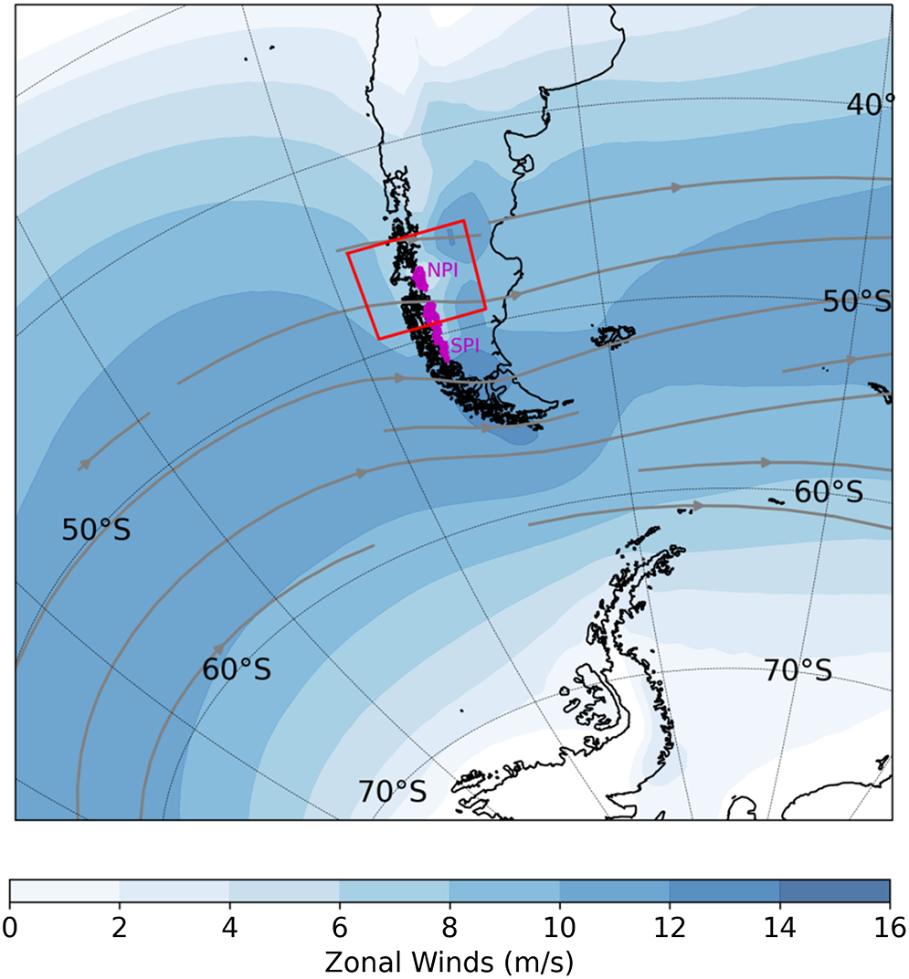

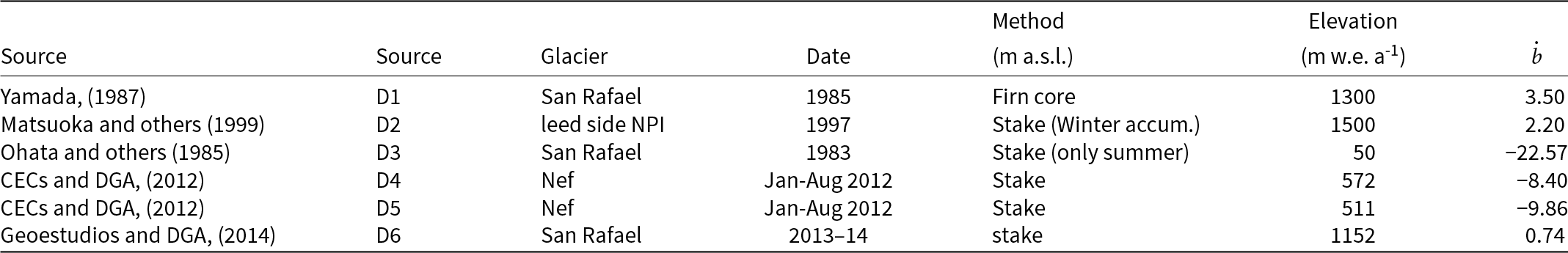
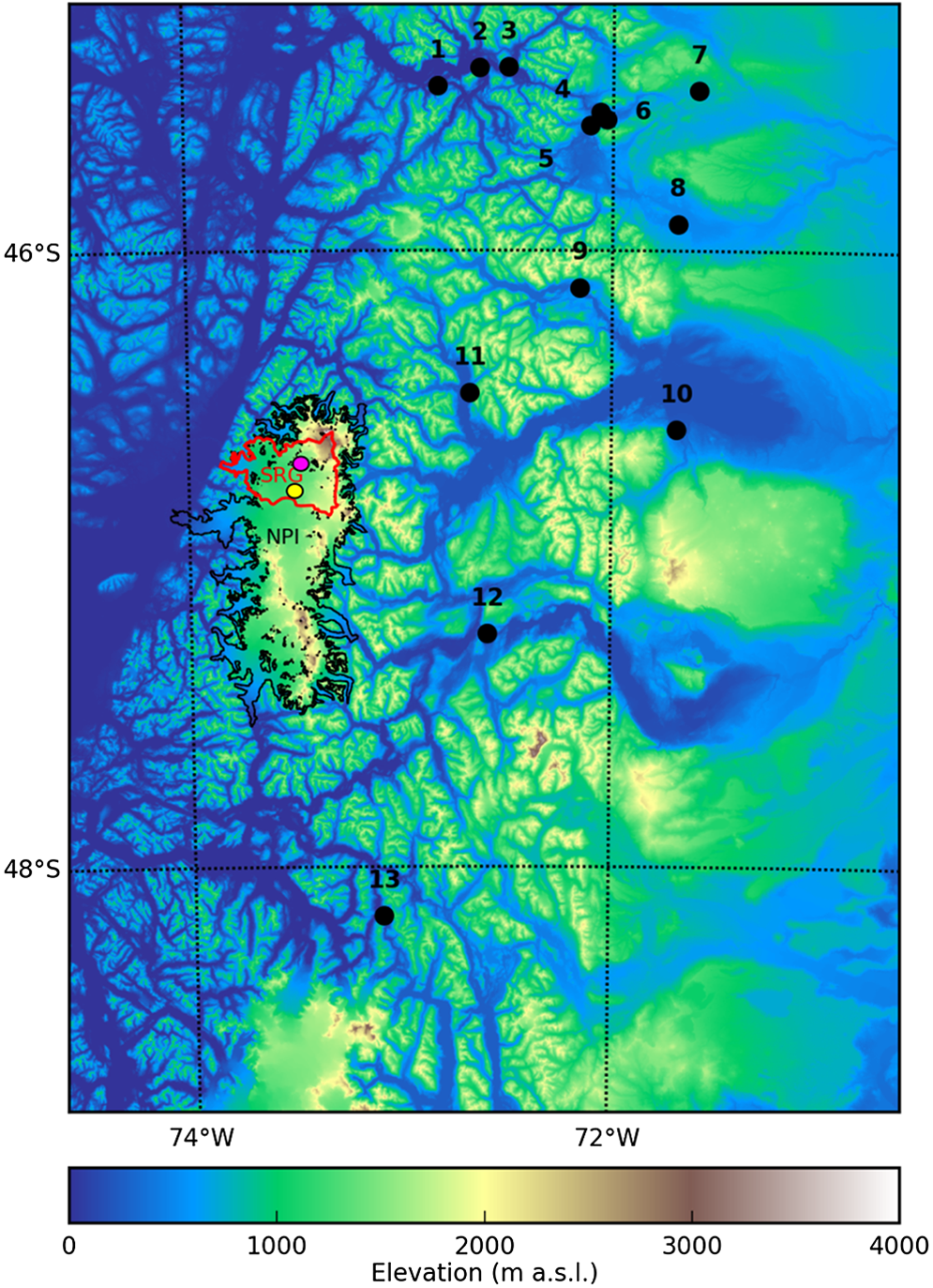
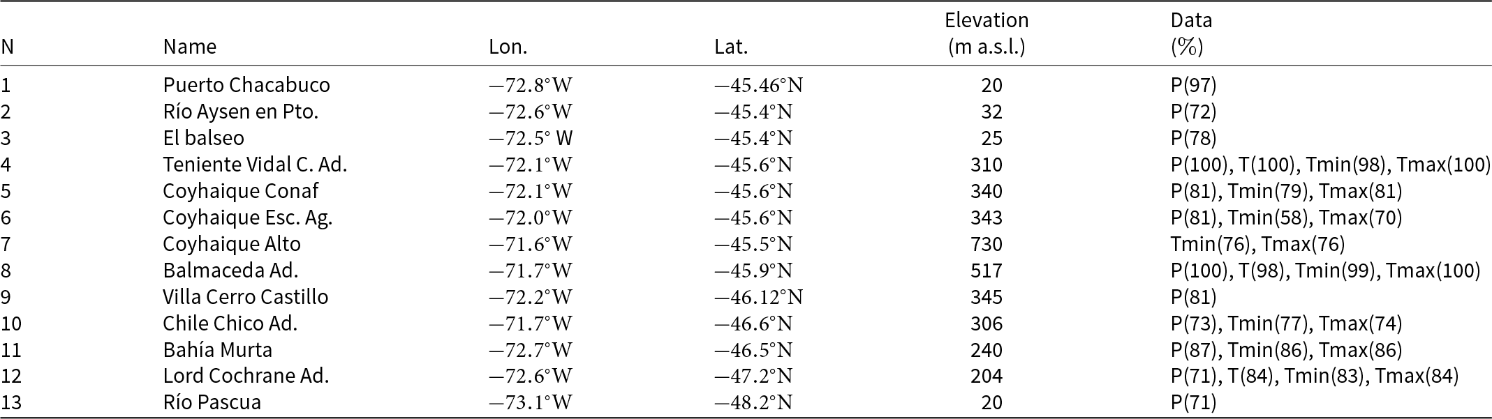

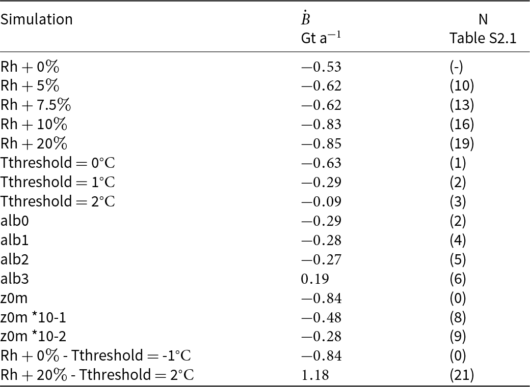
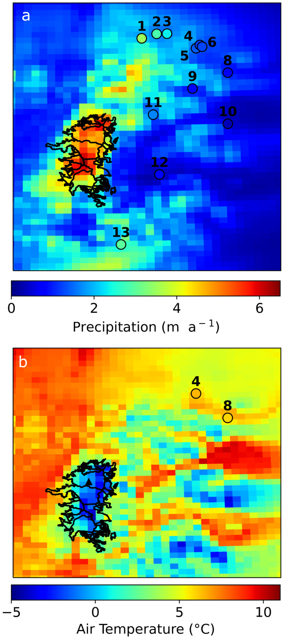
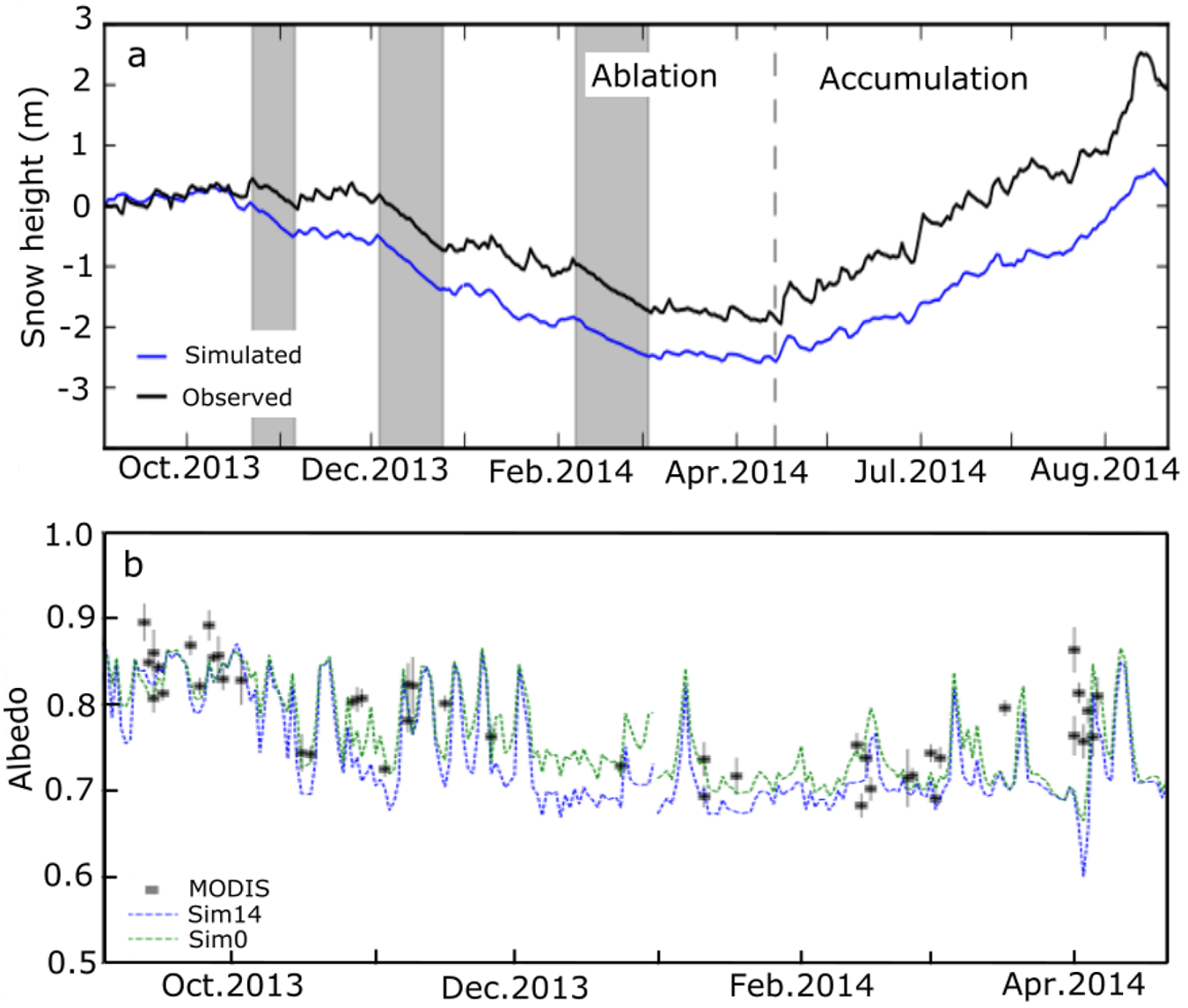

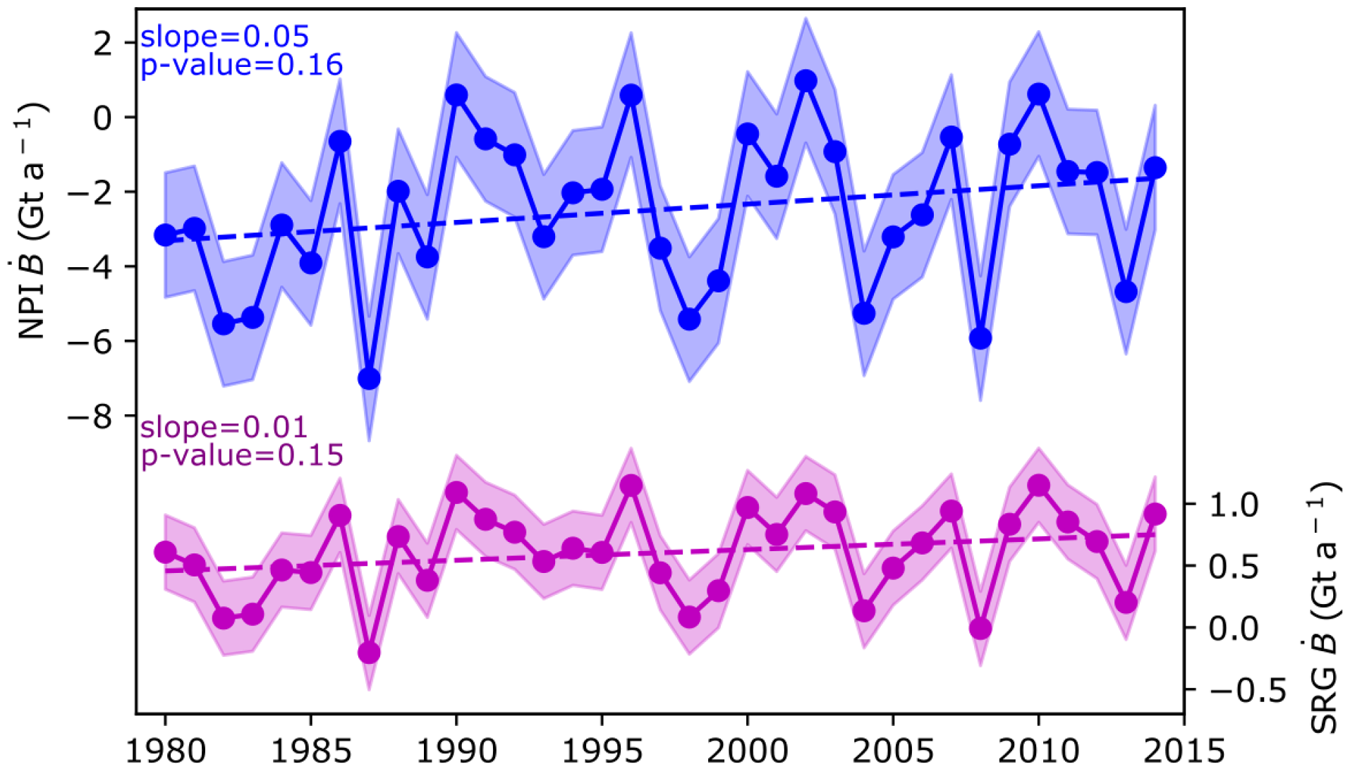
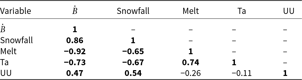
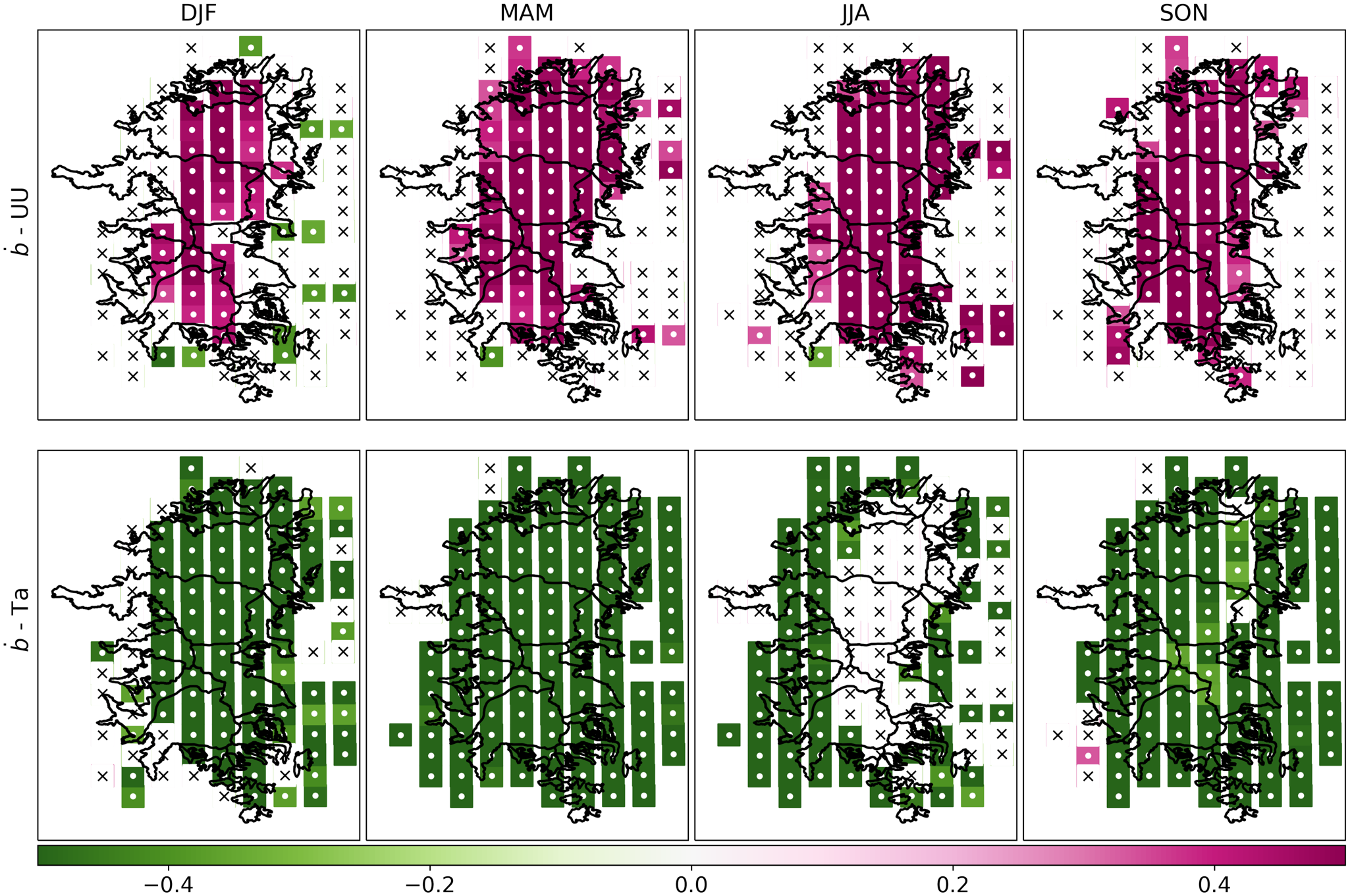
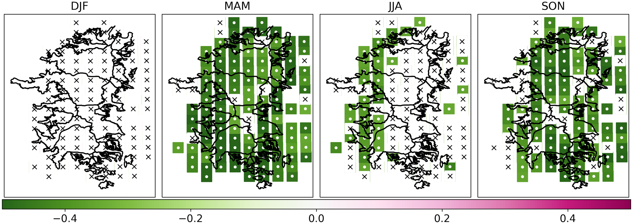
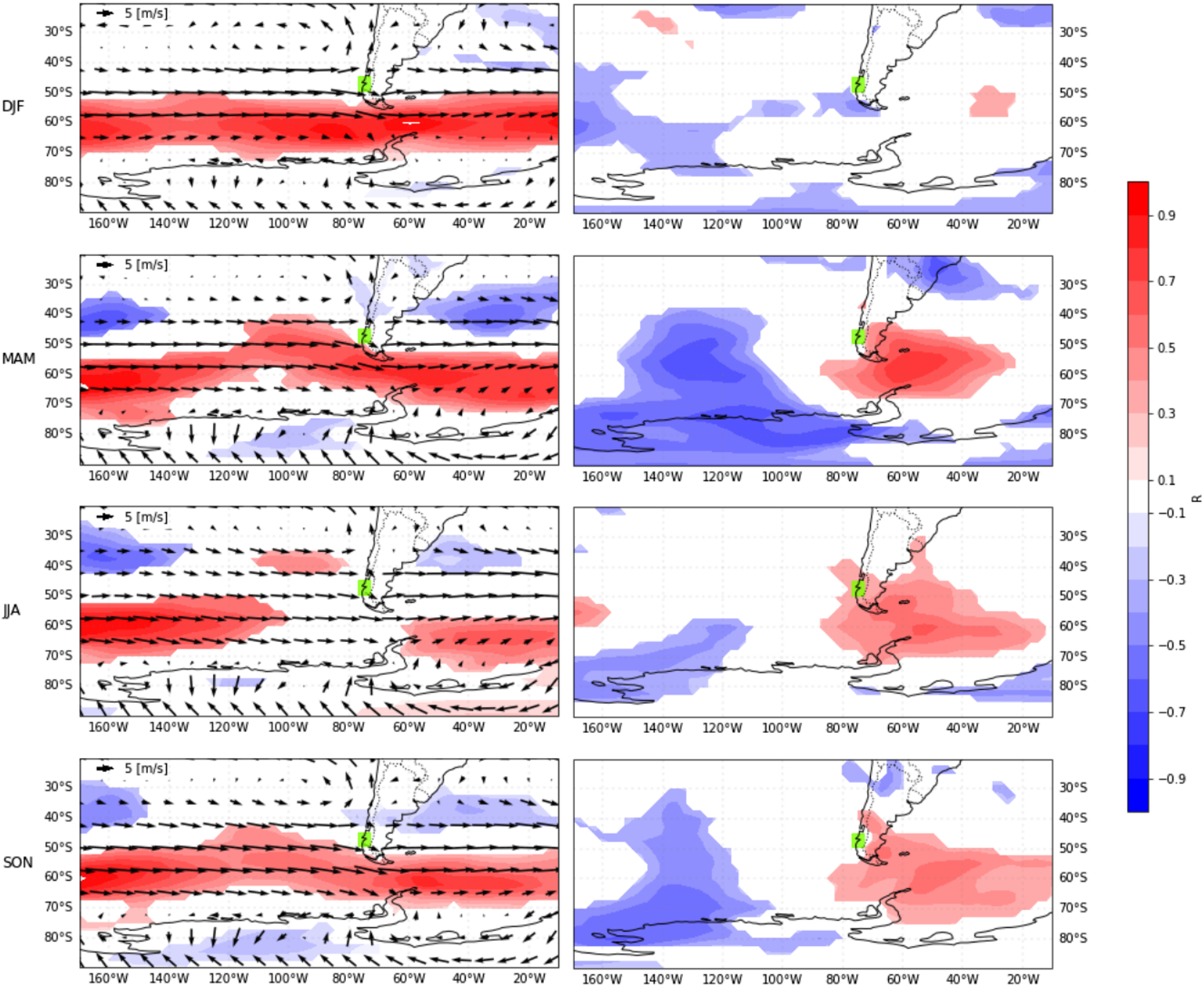
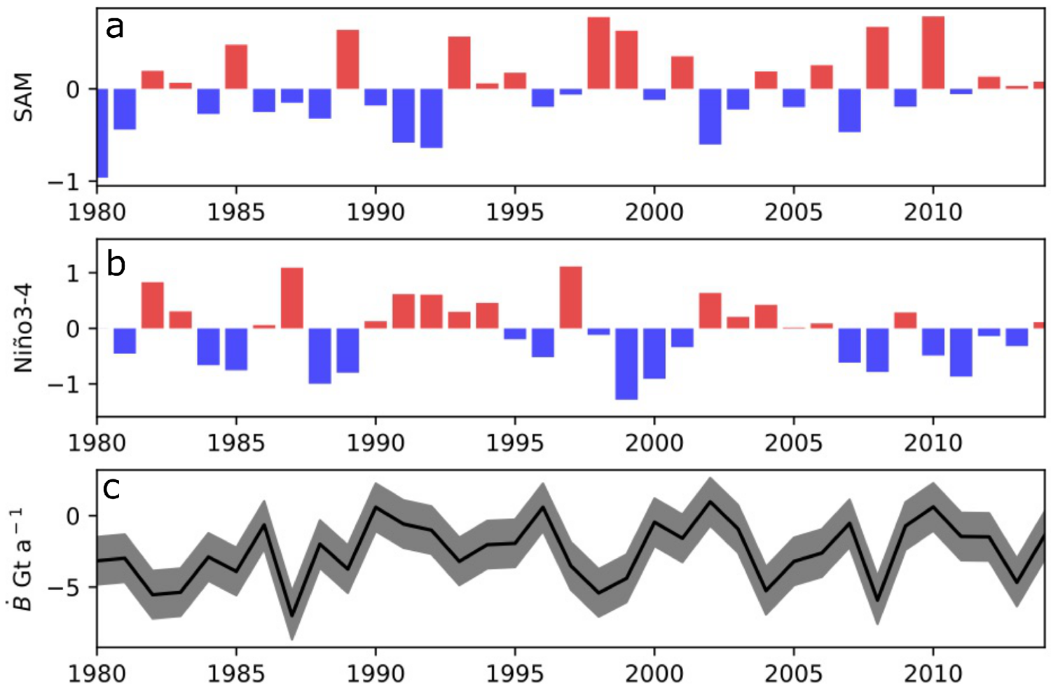
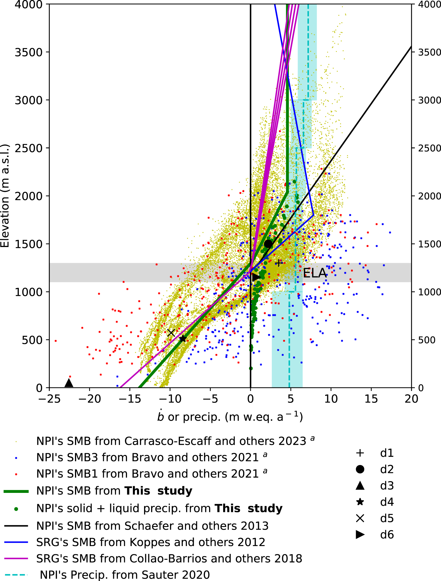
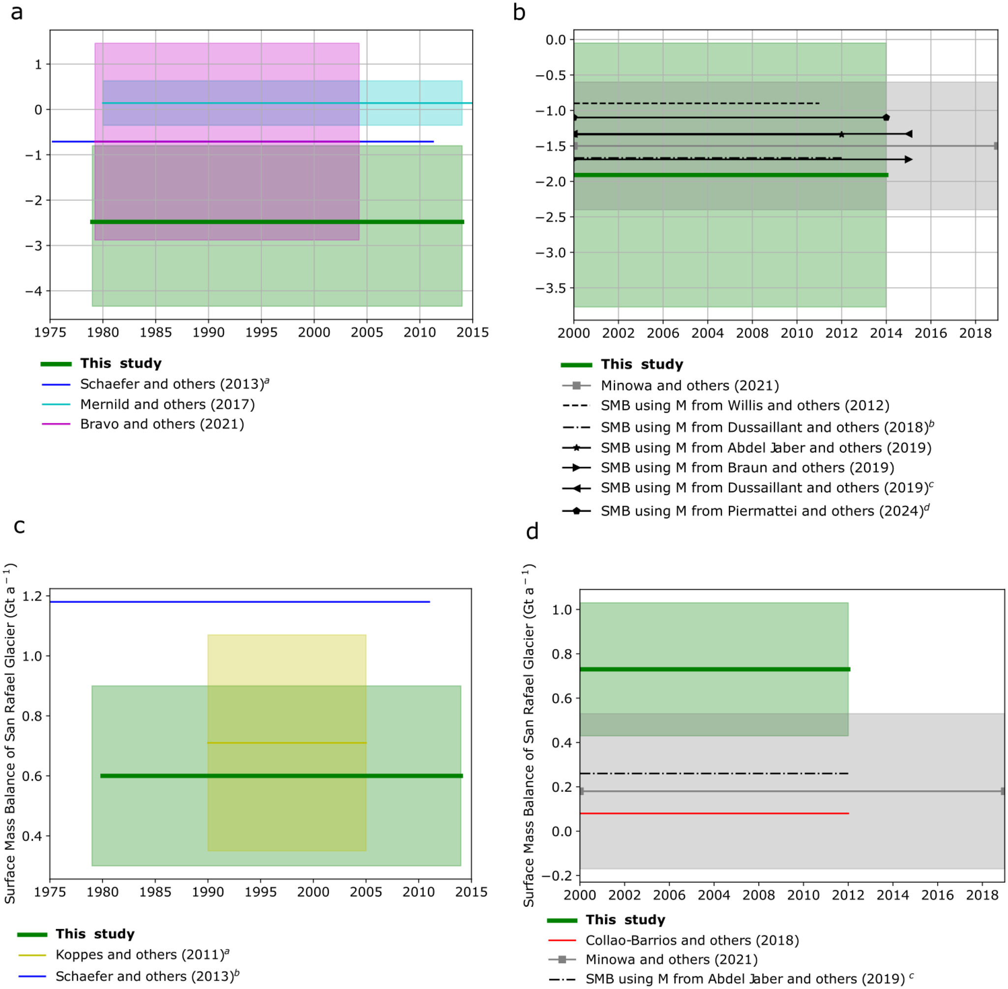


 Open access