Introduction

This research note addresses the question of whether income changes trigger short‐term effects on political involvement.¹ A large literature has reported lower political involvement among voters with low income or other socio‐economic problems (reviewed e.g. in Dalton, Reference Dalton2017 and Ojeda, Reference Ojeda2018). Such studies, which are predominantly based on cross‐sectional data, often assume that low income triggers social and psychological mechanisms that situationally inhibit political involvement. However, recent scholarship has started addressing the related questions of whether income effects on political involvement are causal and how these effects unfold over time (Prior, Reference Prior2019; Schafer et al., Reference Schafer, Cantoni, Bellettini and Berti Ceroni2021). Based on the observation that political participation often becomes habitual with age and therefore resilient to external influences (Plutzer, Reference Plutzer2002), an emerging literature places economic hardship in the life cycle (Emmenegger et al., Reference Emmenegger, Marx and Schraff2017; Ojeda, Reference Ojeda2018; Prior, Reference Prior2019). A key implication is that cross‐sectional income gaps tend to be confounded with previous experiences and, hence, do not reflect a direct causal effect. That said, the underlying theoretical arguments differ in important ways and the associated empirical evidence remains patchy.

As briefly discussed below, the question of whether short‐term changes in income (or socio‐economic position in general) are able to trigger short‐term reactions in political involvement is theoretically ambiguous and still awaits comprehensive empirical assessment. A problem in the existing literature is that the few longitudinal studies typically rely on just one dataset (and rarely more than three). Given the idiosyncratic features of some panel datasets and contexts, the findings are not always easy to compare. In conjunction with divergent methodological approaches and theoretical foci, this provides a weak basis for knowledge accumulation. We therefore analyse income changes in nine panel datasets from six countries (Germany, the Netherlands, Spain, Switzerland, UK, and the United States). Consistent findings in this reasonably diverse group are more likely to be generalizable to Western democracies than those in previous research. We also wish to highlight this study's achievements in identifying a comparatively large number of panel datasets with political information as an independent contribution to political behaviour research.

Our analysis of individual income trajectories, by far the most comprehensive of its kind, produces an important insight that holds across the covered contexts. Irrespective of method and operationalization, income changes have hardly any predictive power for short‐term changes in the propensity to participate in politics. This holds for voting (intentions) and attitudinal measures of political involvement. Unequal participation, hence, seems to result from stable differences between income groups. As discussed in the conclusions, this is in line with recent research on the contribution of socialization patterns to political inequality.

Existing research on the temporality of income effects

Most research on the link between political involvement and socio‐economic hardship builds on the civic voluntarism model (Schlozman et al., Reference Schlozman, Verba and Brady2012) or Rosenstone's (Reference Rosenstone1982) opportunity‐costs argument. Particularly the latter suggests that, if economic worries occur, the resources for engagement with politics decline immediately. This view has been challenged by studies that explicitly address the temporal dimension of the link between socio‐economic hardship and political involvement. Building on Plutzer (Reference Plutzer2002), Emmenegger et al. (Reference Emmenegger, Marx and Schraff2017) argued and showed with difference‐in‐difference matching in German panel data that unemployment only depresses political interest during the impressionable years of early adulthood. This suggests that the resilience of political habits to economic shocks grows over the life cycle. Ojeda (Reference Ojeda2018) goes in a similar direction. He argued that family income during childhood influences turnout inequality at a young age. The relevance of family background is crowded out by the effect of personal (current) income as people get older. This implies that current income should have direct and more or less immediate effects, at least from prime age onwards. Hence, Ojeda shares the broader point of Emmenegger and colleagues that experiences early in the life course shape participation patterns, but the precise predictions and findings diverge. Unfortunately, the empirical results are difficult to compare because Ojeda largely relied on age‐income interactions in cross‐sectional data and because the dependent variables and countries differed. Moreover, Ojeda's random effects estimators cannot be used to isolate short‐term variability, because they do not decompose within‐ and between‐variation. Prior (Reference Prior2019) used fixed effects and first‐difference models with distributed lags based on British, German, and Swiss panel data to show that income changes have no systematic influence on political interest. While Prior goes beyond the typical focus on just one country, we do not know whether his results hold for other datasets and for other dependent variables, most notably voting. Schafer et al. (Reference Schafer, Cantoni, Bellettini and Berti Ceroni2021) recently found in administrative data from Bologna that the income skew in voting shrinks considerably to a rather small magnitude when stable individual heterogeneity is controlled through a difference‐in‐difference design. Substantive effects were limited to income losses among the (very) poor, which points to potential non‐linearity.

It is worth highlighting that experimental research outside political science provides strong but indirect reasons to suspect direct repercussions of economic worries for political involvement. This research (summarized in Schilbach et al., Reference Schilbach, Schofield and Mullainathan2016, and Sheehy‐Skeffington, Reference Sheehy‐Skeffington2020) has documented impressive short‐term effects of economic scarcity on mental capacities, such as executive control, that are also crucial foundations for political involvement (Holbein & Hillygus, Reference Holbein and Hillygus2020). It hence suggests that income changes could indeed have immediate negative effects through impeding cognitive function. However, such cognitive effects might not equally apply to all facets of political involvement. While they are more likely to influence attitudinal components, such as internal political efficacy, they might not be strong enough to change habitual behaviours, such as voting (Marx & Nguyen, Reference Marx and Nguyen2018). Because previous research did not compare indicators, we know little about whether such differences exist.

In sum, research has only recently sought to causally understand the link between income and political participation by studying its temporal ordering. To date, the literature is far from conclusive on the question of whether income changes can be expected to have direct effects on political involvement. Studies on the topic have often considered individual cases, focused on different dependent variables and tended not to build on each other theoretically. In contrast, we analyse a large number of cases and dependent variables in a unified framework that provides a stronger foundation for knowledge accumulation.

Research strategy

We identified nine panel datasets from six countries that consistently include a range of political dependent variables over time (Table 1). We analyse these data with two main methods (see online Appendices B and C for details). In a first step, we use hybrid random effects models that decompose within‐ and between‐person variation. Practically, this means including for each variable $X$$X$ respondent $i\text{'}s$$i\text{'}\mathrm{s}$ intertemporal mean ${\overline{X}}_i$$\bar{X}_i$ and a de‐meaned predictor $X_{it}-{\overline{X}}_i$$X_{it}-\bar{X}_i$. The latter produces a ‘within‐effect’ which is equivalent to a fixed effects estimator (Bell & Jones, Reference Bell and Jones2015). It thus controls for unobserved time‐constant heterogeneity, but can still be biased by time‐varying confounders.

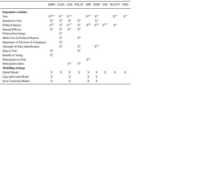
Table 1. Variables for political involvement and modelling strategies by dataset

Notes: BHPS (University of Essex, 2020), GLES (GLES, 2015, 2016, 2019), LISS (Scherpenzeel et al., Reference Scherpenzeel, Marcel, Das, Ester and Kaczmirek2010), POLAT (Hernández et al., Reference Hernández, Galais, Rico, Muñoz, Hierro, Pannico, Barbet, Marinova and Anduiza2021), SHP (SHP Group, 2020), SOEP (SOEP, 2020), GSS (Smith & Schapiro, Reference Smith and Schapiro2017), NLSY97 (Bureau of Labor Statistics, 2019), and PSID (Panel Study of Income Dynamics, 2020).

Superscripted numbers refer to the number of waves the respective variable was surveyed.

* Dummy variable.

^a Combined measure of voting at the next election and support of a political party.

^b Interest in international affairs and in military policy.

Hybrid models are helpful for our research question, because they inform us to what extent income effects are produced by stable differences between persons or by changes over time. They are also relatively undemanding in terms of data structure. A downside pertains to the modelling of the underlying dynamics, which is not necessarily realistic. They assume that income changes between $t_1$$t_1$ and $t_2$$t_2$ fully exert their effect at $t_2$$t_2$. To account for anticipated or delayed effects, we ran additional models with individual fixed effects including lag and lead variables. We pragmatically chose a specification with income lagged by 1, 2, and 3 years as well as a 1‐year lead (assuming that income changes are rarely anticipated far into the future). This reduced the number of datasets we could include in the analysis (Table 1).

As a robustness check, we use error correction models (ECM) as a third alternative to model panel dynamics (De Boef & Keele, Reference De Boef and Keele2008). As discussed in online Appendix I, ECMs reflect the theoretical possibility of a long‐term equilibrium in the income‐participation link, which is temporarily upset through short‐term income changes. ECMs allow analysing whether there are short‐term deviations and, if yes, whether and how quickly there is a return to the equilibrium. On the flip side, these models are considerably more difficult to estimate than hybrid or lags‐and‐leads models because including lags of the dependent variable inevitably violates the exogeneity assumption (see online Appendix I for details).

Data

We include data from the British Household Panel Study/Understanding Society (BHPS/UKHLS), the German Longitudinal Election Study (GLES) and Socio‐Economic Panel (GSOEP), the Dutch Longitudinal Internet Studies for the Social Sciences (LISS), the Spanish Political Attitudes Panel (POLAT), the Swiss Household Panel (SHP) and, from the United States, the Panel Study of Income Dynamics (PSID), the National Longitudinal Survey of Youth (NLSY97) and the General Social Survey Panels (GSS). All surveys allowed us to estimate the hybrid models. We had to restrict the estimation of the more demanding lags‐and‐leads models to the BHPS/UKHLS, LISS, SHP and SOEP.

We measured political involvement flexibly with a diverse range of variables (see Table 1), depending on availability in the datasets. We acknowledge that these variables capture distinct aspects of political involvement. The broad approach accounts for the possibility that attitudinal indicators might be more responsive than political dispositions or behaviours. It hence maximizes the chances to detect effects of income changes.

As explanatory variables, we used both objective and subjective income measures in different operationalizations.² The details are discussed in online Appendix J. In the models with individual fixed effects, we additionally modelled income shocks as dummy variables that take the value of 1 if a person experiences an income reduction between $t_{-1}$$t_{-1}$ and $t_0$$t_0$ of at least two deciles.

We controlled for age, education and labour force status in all models, and for sex and migration status in the hybrid models (plus race in the US data). With the exception of age and objective income, all quasi‐metric variables were recoded to a scale from 0 to 10. For binary dependent variables, we use linear probability models.³

Findings

Within‐ and between‐effects of income on political involvement

Figure 1 displays results of hybrid random effects models in which income is operationalized in deciles of equivalized household income. Although there is some variation across countries and variables, the decomposition yields a clear picture. The income gradient is driven by differences between individuals, while there are little to no effects for within‐person change.

Figure 1. Within‐ and between effects of income on political participation. [Colour figure can be viewed at wileyonlinelibrary.com]

Notes: Results for ‘Vote’ (all datasets), ‘Political Interest’ (LISS), ‘Has party ID’ (GLES, SOEP, POLAT) and all variables in the GSS are performed using linear probability models. For readability, we rescaled their coefficients so that they indicate the effect of going from the lowest to the highest income decile. All other coefficients show the effect of a one‐income‐decile change on dependent variables scaled 1 to 10.

To begin with voting participation, all seven coefficients indicate significant and substantial between‐effects. For better readability, we rescaled the coefficients for voting (and all other binary variables) so that they indicate changes from the lowest to the highest decile. Respondents from the highest income decile are between eight (LISS) and 23 percentage points (SOEP) more likely to vote than respondents from the lowest income decile. At the same time, a within‐person change from the lowest to highest income decile has either no effect or a very small one (e.g. a 1.2 percentage point increase in the SHP). The same pattern holds for intention to vote in the BHPS/UKHLS and the LISS. In both German datasets, however, there are significant but small within‐effects on voting intention of 0.04 (GLES) and 0.06 (SOEP) point changes for a one‐decile change (recall that all continuous dependent variables are rescaled to a range from 1 to 10). Again, these within‐effects are smaller than the corresponding between‐effects. The only dataset showing no significant between‐effect is the Spanish POLAT.

Political interest likewise shows substantial between‐effects, ranging from a 0.08 (GLES) to 0.16 (SHP) point change for a one‐decile income change. There are similar effects in the GSS, where respondents were asked about their interest in international and military affairs. Respondents in the highest income decile are about 23 percentage points more likely to be at least moderately interested in international affairs than those from the lowest income decile. Yet again, there is virtually no effect for income changes over time. Only in the case of the SOEP do we find a small and negative significant effect (−0.02).

This pattern continues for attitudinal indicators of political involvement, like internal efficacy, having a party identification and party identification strength. We also included a number of less common indicators, like the number of polls someone usually participated in during the previous year (SHP), an index of non‐electoral political participation (LISS), the subjective importance of elections and election campaigns (GLES), the subjective duty to vote and the personal benefits of voting (BHPS/UKHLS). In all cases, we find broadly the same patterns described above. The same is true for indices of political media use (GLES and POLAT) and political knowledge (GLES).

Lags and leads of income changes

In a next step, we relaxed the (possibly unrealistic) assumption that the effect of income change unfolds fully in the following wave. The results in Figure 2 show that even if we account with lags and leads for anticipation and gradually unfolding effects, there is no evidence that would challenge our findings from the hybrid models. The experience of an income shock has a substantially negligible effect in the BHPS and UKHLS data; it merely decreases the probability to vote by one percentage point in the same period ( $t_0$$t_0$) and by even less in $t_{+1}$$t_{+1}$ (0.7 percentage points). There is no anticipation effect in the sense that citizens' voting probability decreases when they expect a substantial drop in income. We also find no effect across all periods in the LISS and SHP.

Figure 2. Fixed effects models including lagged and leaded predictors. [Colour figure can be viewed at wileyonlinelibrary.com]

Notes: The figure shows the effects of an income drop of at least two deciles compared to the previous period in $t_0$$t_0$ as well as the effects of lags and leads of this income drop. All models include individual fixed effects. Results for the binary variables ‘Vote’ (all datasets), ‘Political Interest’ (LISS) and ‘Has party ID’ (SOEP) are based on linear probability models.

This pattern largely holds for political interest. While there are a few significant effects, they do not add up to any consistent pattern across countries. In the UK, there is a drop of 0.05 units in $t_0$$t_0$ followed by another 0.04 units in $t_{+3}$$t_{+3}$. In the SOEP, by contrast, we find a 0.04 drop in political interest in $t_{-1}$$t_{-1}$. Nevertheless, there are no changes in political interest when or after such a shock occurs. Analyses of the LISS data show that individuals experienced a slight increase of 2.8 percentage points in the probability of being fairly or very interested in politics in $t_{-1}$$t_{-1}$. Finally, analyses of the Swiss data show only a minor effect in $t_{+1}$$t_{+1}$ (−0.05).

We find similar patterns with mostly null effects for a wide range of other indicators of political involvement. The few effects that we find are inconsistent and small given that the continuous dependent variables are measured on scales from 0 to 10.

Robustness checks

As robustness checks, we ran both types of models with explanatory variables based on raw income, logged income and income satisfaction. We also tested the effects of job loss since the last wave.⁴ In addition, we generated multi‐item scales for political involvement in each country. The results are substantially similar to the models reported here. No operationalization produces a consistent effect of income changes (online Appendices B, C, F and G). Also in error correction models, we find only small effects of income changes, if any (online Appendix I). Finally, equivalence tests (Lakens, Reference Lakens2017) strongly suggest the absence of meaningful effects. As shown in online Appendix B, most 90% confidence intervals do not overlap with an extremely conservative ‘smallest effect size of interest’ of 0.1 or even 0.05.⁵

Individual heterogeneity by age, income and political involvement

Could our non‐findings be explained by diverging patterns across sub‐groups? First, income shocks might differ by age group. While Emmenegger et al. (Reference Emmenegger, Marx and Schraff2017) suggest that their importance should decrease with age, Ojeda's (Reference Ojeda2018) argument implies that they should increase. To assess the interaction of age and income, we included the product of both variables in our hybrid models (de‐meaned and as inter‐temporal mean). In almost all cases, the interactions proved to be insignificant or substantially negligible. Table 2 provides an exemplification for voting participation, but the results are similar for other indicators of political involvement across datasets. Hence, based on this operationalization, there is no evidence for life‐cycle variation in the responsiveness to income changes.

Table 2. Overview of interaction effects for age and income on vote in hybrid models

Notes: Income is measured as equivalized household income in deciles from 1 to 10. Age in years is centred at the age of 18. W indicates within effects, B refers to between effects. Standard errors in parentheses.

* $p<0.05$$p &#x003C; 0.05$, ** $p<0.01$$p &#x003C; 0.01$, *** $p<0.001$$p &#x003C; 0.001$.

Second, income shocks might be more relevant for respondents with already low income (Pacheco & Plutzer, Reference Pacheco and Plutzer2008; Rosenstone, Reference Rosenstone1982). We analysed this possibility by breaking down the ‘shock’ dummy into a multi‐category variable. Compared to the previous period, respondents in this operationalization can either experience an income increase, stability or a one‐decile drop (irrespective of previous income). In addition, we added separate outcomes in the form of a two‐decile drop (or more) from (a) the upper half of the income distribution, (b) decile four and (c) decile three. Stronger effects at the bottom of the income distribution should be captured by categories (b) and (c). Because of the smaller categories, we needed a larger sample and therefore restricted the analysis to the British data. Large income drops at the bottom of the distribution have equally small and insignificant effects on voting and political interest (online Appendix H).

Finally, the detrimental effects of income shocks might be restricted to respondents with low initial political involvement, who lack the stabilizing force of habituation. To address this possibility, we followed the same procedure as for the age‐income interaction, but this time multiplying income with political interest lagged by two periods. We used this model to predict voting in a hybrid model, again, only in the British data. Lagging political interest by two waves should ensure that we condition on pre‐shock involvement. Again, the interaction effect turned out to be insignificant (online Appendix H).

Conclusions

This article has provided the most comprehensive analysis to date of how income and political involvement are related in longitudinal data. Our study uses many datasets, specifications and operationalizations, which helps us to avoid over‐interpreting chance findings and provides a stronger basis for at least tentative generalization.

Indeed, we found a number of effects for single variables that might look relevant in isolation. However, our encompassing analysis has mostly revealed them to be outliers in the broader picture. This picture suggests that the answer to our research question is a resounding no. We clearly find that income changes do not influence political involvement. We also find no evidence that young people are more or less responsive to income changes. The same is true for low‐income earners and respondents with low initial interest in politics.

In sum, we see this article as a step towards consolidating knowledge on important research questions that so far have received a rather disparate treatment. While it confirms some previous analyses, it challenges others. Most clearly, our results confirm Prior's (Reference Prior2019) finding that income does not affect political interest, but generalizes it to a considerably larger number of countries and, crucially, measures of political involvement. Taken together, our results and Prior's (Reference Prior2019) results strongly support the theoretical position that political involvement is habitual and hardly influenced by short‐term income changes. The often‐reported negative correlation between income and voting is likely to reflect stable differences between income groups. This interpretation is consistent with arguments about the long‐term consequences of unequal political socialization (Emmenegger et al., Reference Emmenegger, Marx and Schraff2017; Ojeda, Reference Ojeda2018).

However, we could not generalize the argument by Emmenegger et al. (Reference Emmenegger, Marx and Schraff2017) about the ‘impressionable years’ as a period of heightened responsiveness to socio‐economic shocks. We did not detect a significant interaction between young age and income changes as predictors of political involvement. A possible reason for the diverging findings is that Emmenegger et al. (Reference Emmenegger, Marx and Schraff2017) focused on youth unemployment, which might have distinct socio‐emotional repercussions. Our findings are also inconsistent with Ojeda's (Reference Ojeda2018) argument that the importance of personal income increases over the life course. We do acknowledge, however, that the question of life‐course variation deserves treatment in a separate paper in which finer‐grained methods can be explored.

Another possible extension of our analysis would be moving from income effects to poverty and other acute socio‐economic problems. Recent analyses by Schafer et al. (Reference Schafer, Cantoni, Bellettini and Berti Ceroni2021) and Schaub (Reference Schaub2021) suggest that intense hardship in specific groups might produce more immediate effects on voting. While we could not detect any non‐linearity, this aspect certainly warrants more attention. This is even more so as self‐reported income is often distorted by measurement error (Schafer et al., Reference Schafer, Cantoni, Bellettini and Berti Ceroni2021), a potentially serious limitation of our approach (which we could only partially remedy by including subjective income). Future research should therefore explore more concrete indicators of economic hardship that are independent of self‐reported income.

Do our findings imply that income is irrelevant for political involvement? We believe this conclusion would be premature. Between‐effects of income are likely inflated due to unobserved heterogeneity. However, the relevant unobserved factors could themselves be shaped by income differences. As mentioned above, this would be the case if, for instance, parental income in adolescence influences political socialization, which crystallizes into stable patterns with age (Akee et al., Reference Akee, Copeland, Holbein and Simeonova2020; Plutzer, Reference Plutzer2002; Schlozman et al., Reference Schlozman, Verba and Brady2012). Based on our data, we cannot rule out that income‐related processes within the family prior to voting age already interfere with political socialization. Exploring this possibility is a logical next step for research on political inequality.