


1 Introduction
Mathematicians love classifications. We enjoy classifying objects into different categories, and for a good reason. Classifications teach us about abstract properties and help us deepen our understanding of various objects and theories.
Set theorists are generally interested in models of set theory. If V satisfies
 $\mathsf {ZFC}$
, we want to classify models of set theory which lie between V and some generic extension,Footnote
1
$\mathsf {ZFC}$
, we want to classify models of set theory which lie between V and some generic extension,Footnote
1
 $V[G]$
. In the case where “set theory” is understood as
$V[G]$
. In the case where “set theory” is understood as
 $\mathsf {ZFC}$
, Vopěnka’s theorem tells us exactly what the intermediate models are: they are generic extensions given by subforcings of the forcing which is used to introduce G over V.
$\mathsf {ZFC}$
, Vopěnka’s theorem tells us exactly what the intermediate models are: they are generic extensions given by subforcings of the forcing which is used to introduce G over V.
On the other hand, when we are interested in classifying arbitrary intermediate models of
 $\mathsf {ZF}$
, instead, even if we assume that V satisfied
$\mathsf {ZF}$
, instead, even if we assume that V satisfied
 $\mathsf {ZFC}$
, the task becomes significantly harder, and dare we say, nigh impossible. For a start, a generic extension of a model of
$\mathsf {ZFC}$
, the task becomes significantly harder, and dare we say, nigh impossible. For a start, a generic extension of a model of
 $\mathsf {ZFC}$
cannot be a model of
$\mathsf {ZFC}$
cannot be a model of
 $\mathsf {ZF}+\lnot \mathsf {AC}$
. One might be inclined to say that such intermediate extension would still be a symmetric extension, which is a type of inner model of a generic extension defined using automorphisms of the forcing. While this is true under some additional conditions on the intermediate model, it turns out that if M is an intermediate model between V and
$\mathsf {ZF}+\lnot \mathsf {AC}$
. One might be inclined to say that such intermediate extension would still be a symmetric extension, which is a type of inner model of a generic extension defined using automorphisms of the forcing. While this is true under some additional conditions on the intermediate model, it turns out that if M is an intermediate model between V and
 $V[G]$
, even if M is a symmetric extension of V, it might not be given by any forcing even remotely related to the one for which G was generic.
$V[G]$
, even if M is a symmetric extension of V, it might not be given by any forcing even remotely related to the one for which G was generic.
The reality is that intermediate models of
 $\mathsf {ZF}$
are far wilder than their
$\mathsf {ZF}$
are far wilder than their
 $\mathsf {ZFC}$
-counterparts. The Bristol model is the first explicit example of such a model. This is a model intermediate to
$\mathsf {ZFC}$
-counterparts. The Bristol model is the first explicit example of such a model. This is a model intermediate to
 $L[c]$
, where c is an L-generic Cohen real, which is not
$L[c]$
, where c is an L-generic Cohen real, which is not
 $L(x)$
for any set x, let alone a symmetric extension of L (by any means, not just the Cohen forcing). While there is a semi-canonical Bristol model, modulo a particular choice of c, it is immediate from the construction that, in a very good sense of the word, most models intermediate to
$L(x)$
for any set x, let alone a symmetric extension of L (by any means, not just the Cohen forcing). While there is a semi-canonical Bristol model, modulo a particular choice of c, it is immediate from the construction that, in a very good sense of the word, most models intermediate to
 $L[c]$
are not even definable. We will clarify this in Section 7.
$L[c]$
are not even definable. We will clarify this in Section 7.
The idea for this model came about in a small 2011 workshop in Bristol on topics related to the HOD Conjecture. In attendance were Andrew Brooke-Taylor, James Cummings, Moti Gitik, Menachem Magidor, Ralf Schindler, Matteo Viale, Philip Welch, and W. Hugh Woodin, henceforth “the Bristol group”. The details were not written down in full, and the model remained as a folklore rumour until the author’s effort to formalise it. The details of the construction are given in [Reference Karagila8], which was part of the author’s Ph.D. dissertation, written under the supervision of Menachem Magidor. This article aims to give a bird’s eye view of the construction, from three different perspectives (for people coming from different walks of set theory). We will also correct a few minor mistakes in the original paper, and prove a handful of new theorems about the Bristol model, and about models of
 $\mathsf {ZF}$
in general.
$\mathsf {ZF}$
in general.
1.1 Structure of this article
The Bristol model is presented in [Reference Karagila8] as an iteration of symmetric extensions, starting from a Cohen real. The idea is to have, at successor steps, a “decoding mechanism” which is a symmetric extension over an intermediate step such that two properties hold: (1) the decoding mechanism has a generic (relative to the intermediate step) in the Cohen extension and (2) the decoding mechanism only adds subsets of sufficiently high rank.
We will cover the basics of the technical tools in Section 2. We will define symmetric extensions, and briefly outline the main ideas related to iterating them (or rather, why it is hard to iterate symmetric extensions). We will also discuss the combinatorial ideas needed for the decoding mechanism, both at successors of limits, as well as double successors.
After covering the preliminary tools, we will present the decoding mechanism, and the generic argument needed for the proof to work. In Section 4 we explain the three different approaches to constructing the Bristol model. All three are equivalent, but for different people some of these might be seen as “more natural” and can help understand the model better. We will not dive into the intimate details, though. The goal of this article is to serve as a companion, and help provide not only the big picture of the construction, but also serve as a first step towards reading and understanding the construction’s details presented in [Reference Karagila8].
Having discussed the construction of the model, we will then point towards some minor gaps and typos in the original [Reference Karagila8]. Then we will discuss Kinna–Wagner Principles which we expect to play a role in the study of choiceless models such as the Bristol model. We will make some new observations, and suggest conjectures for future research. Finally, in Section 9 we will prove that some sets in the Bristol model cannot be linearly ordered, and therefore the Boolean Prime Ideal theorem is false there. We finish the article with a long list of open questions related to the Bristol model.
2 Preliminaries: Symmetric extensions, their iterations, and more
In this article, the term forcing will denote a preordered set with a maximum, denoted by ![]() , unless explicitly mentioned otherwise.Footnote
2
Of course, we will invariably think about a forcing as a partially ordered set, a separative one, in fact, knowing full well that this will not limit our generality.Footnote
3
The elements of
, unless explicitly mentioned otherwise.Footnote
2
Of course, we will invariably think about a forcing as a partially ordered set, a separative one, in fact, knowing full well that this will not limit our generality.Footnote
3
The elements of
 ${\mathbb {P}}$
are called conditions, and using them we define
${\mathbb {P}}$
are called conditions, and using them we define
 ${\mathbb {P}}$
-names. We refer the reader to any of [Reference Halbeisen4, Reference Jech6, Reference Kunen12] for the basic methodology of forcing.
${\mathbb {P}}$
-names. We refer the reader to any of [Reference Halbeisen4, Reference Jech6, Reference Kunen12] for the basic methodology of forcing.
Let
 ${\mathbb {P}}$
be a notion of forcing, we follow the convention that if
${\mathbb {P}}$
be a notion of forcing, we follow the convention that if
 $p,q\in {\mathbb {P}}$
, then
$p,q\in {\mathbb {P}}$
, then
 $q\leq p$
indicates that q is a stronger condition, and we will often say that q extends p. Two conditions are compatible if they have a common extension, and they are incompatible otherwise.
$q\leq p$
indicates that q is a stronger condition, and we will often say that q extends p. Two conditions are compatible if they have a common extension, and they are incompatible otherwise.
Given a collection of
 ${\mathbb {P}}$
-names,
${\mathbb {P}}$
-names,
 $\{\dot x_i\mid i\in I\}$
, that we want to transform into a name, we will denote by
$\{\dot x_i\mid i\in I\}$
, that we want to transform into a name, we will denote by
 $\{\dot x_i\mid i\in I\}^\bullet $
the name
$\{\dot x_i\mid i\in I\}^\bullet $
the name ![]() , and we say that a name is a
, and we say that a name is a
 $\bullet $
-name when it has this form. This extends naturally to ordered pairs, sequences, functions, etc. With this notation we can easily define the canonical names for ground model sets:
$\bullet $
-name when it has this form. This extends naturally to ordered pairs, sequences, functions, etc. With this notation we can easily define the canonical names for ground model sets:
 $\check x=\{\check y\mid y\in x\}^\bullet $
.
$\check x=\{\check y\mid y\in x\}^\bullet $
.
Given two
 ${\mathbb {P}}$
-names,
${\mathbb {P}}$
-names,
 $\dot x$
and
$\dot x$
and
 $\dot y$
, we say that
$\dot y$
, we say that
 $\dot x$
appears in
$\dot x$
appears in
 $\dot y$
if there is some
$\dot y$
if there is some
 $p\in {\mathbb {P}}$
such that
$p\in {\mathbb {P}}$
such that
 $\langle p,\dot x\rangle \in \dot y$
. We will use a similar terminology stating that p appears in
$\langle p,\dot x\rangle \in \dot y$
. We will use a similar terminology stating that p appears in
 $\dot y$
.
$\dot y$
.
2.1 Symmetric extensions
As we remarked, a generic extension of a model of
 $\mathsf {ZFC}$
is again a model of
$\mathsf {ZFC}$
is again a model of
 $\mathsf {ZFC}$
. Symmetric extensions are intermediate models to generic extensions where the axiom of choice may fail.
$\mathsf {ZFC}$
. Symmetric extensions are intermediate models to generic extensions where the axiom of choice may fail.
Let
 ${\mathbb {P}}$
be a forcing, and let
${\mathbb {P}}$
be a forcing, and let
 $\pi $
be an automorphism of
$\pi $
be an automorphism of
 ${\mathbb {P}}$
. The action of
${\mathbb {P}}$
. The action of
 $\pi $
extends to the
$\pi $
extends to the
 ${\mathbb {P}}$
-names by recursion:
${\mathbb {P}}$
-names by recursion:
 $$\begin{align*}\pi\dot x=\{\langle\pi p,\pi\dot y\rangle\mid\langle p,\dot y\rangle\in\dot x\}.\end{align*}$$
Lemma (The Symmetry Lemma).
Let
 $\pi $
be an automorphism of a forcing
$\pi $
be an automorphism of a forcing
 ${\mathbb {P}}$
, and let
${\mathbb {P}}$
, and let
 $\dot x$
be a
$\dot x$
be a
 ${\mathbb {P}}$
-name. For every condition p,
${\mathbb {P}}$
-name. For every condition p,
 $$\begin{align*}p\mathrel{\Vdash}\varphi(\dot x)\iff\pi p\mathrel{\Vdash}\varphi(\pi\dot x).\end{align*}$$
Fix a group
 ${\mathscr {G}}\leq \operatorname {\mathrm {Aut}}({\mathbb {P}})$
. We say that
${\mathscr {G}}\leq \operatorname {\mathrm {Aut}}({\mathbb {P}})$
. We say that
 ${\mathscr {F}}$
is a filter of subgroups on
${\mathscr {F}}$
is a filter of subgroups on
 ${\mathscr {G}}$
if it is a filter on the lattice of subgroups, namely, it is a non-empty collection of subgroups which is closed under finite intersections and supergroups. We will, unless stated otherwise, assume that it is a proper filter, i.e., the trivial group is not in
${\mathscr {G}}$
if it is a filter on the lattice of subgroups, namely, it is a non-empty collection of subgroups which is closed under finite intersections and supergroups. We will, unless stated otherwise, assume that it is a proper filter, i.e., the trivial group is not in
 ${\mathscr {F}}$
.Footnote
4
Finally,
${\mathscr {F}}$
.Footnote
4
Finally,
 ${\mathscr {F}}$
is normal if whenever
${\mathscr {F}}$
is normal if whenever
 $\pi \in {\mathscr {G}}$
and
$\pi \in {\mathscr {G}}$
and
 $H\in {\mathscr {F}}$
, then
$H\in {\mathscr {F}}$
, then
 $\pi H\pi ^{-1}\in {\mathscr {F}}$
as well. In most cases we are interested not necessarily in a filter, but in a filter base, and we will ignore the distinction between the two.
$\pi H\pi ^{-1}\in {\mathscr {F}}$
as well. In most cases we are interested not necessarily in a filter, but in a filter base, and we will ignore the distinction between the two.
Call
 $\langle {\mathbb {P}},{\mathscr {G}},{\mathscr {F}}\rangle $
a symmetric system if
$\langle {\mathbb {P}},{\mathscr {G}},{\mathscr {F}}\rangle $
a symmetric system if
 ${\mathbb {P}}$
is a notion of forcing,
${\mathbb {P}}$
is a notion of forcing,
 ${\mathscr {G}}$
is a group of automorphisms of
${\mathscr {G}}$
is a group of automorphisms of
 ${\mathbb {P}}$
, and
${\mathbb {P}}$
, and
 ${\mathscr {F}}$
is a normal filter of subgroups on
${\mathscr {F}}$
is a normal filter of subgroups on
 ${\mathscr {G}}$
. We shall fix a symmetric system
${\mathscr {G}}$
. We shall fix a symmetric system
 $\langle {\mathbb {P}},{\mathscr {G}},{\mathscr {F}}\rangle $
for the rest of this section.
$\langle {\mathbb {P}},{\mathscr {G}},{\mathscr {F}}\rangle $
for the rest of this section.
For a
 ${\mathbb {P}}$
-name,
${\mathbb {P}}$
-name,
 $\dot x$
, let
$\dot x$
, let
 $\operatorname {\mathrm {sym}}_{\mathscr {G}}(\dot x)$
denote the group
$\operatorname {\mathrm {sym}}_{\mathscr {G}}(\dot x)$
denote the group
 $\{\pi \in {\mathscr {G}}\mid \pi \dot x=\dot x\}$
. If it is the case that
$\{\pi \in {\mathscr {G}}\mid \pi \dot x=\dot x\}$
. If it is the case that
 $\operatorname {\mathrm {sym}}_{\mathscr {G}}(\dot x)\in {\mathscr {F}}$
, then we say that
$\operatorname {\mathrm {sym}}_{\mathscr {G}}(\dot x)\in {\mathscr {F}}$
, then we say that
 $\dot x$
is
$\dot x$
is
 ${\mathscr {F}}$
-symmetric. And similarly, we say that
${\mathscr {F}}$
-symmetric. And similarly, we say that
 $\dot x$
is hereditarily
$\dot x$
is hereditarily
 ${\mathscr {F}}$
-symmetric if being
${\mathscr {F}}$
-symmetric if being
 ${\mathscr {F}}$
-symmetric is hereditarily true for all names hereditarily appearing in
${\mathscr {F}}$
-symmetric is hereditarily true for all names hereditarily appearing in
 $\{\dot x\}^\bullet $
.
$\{\dot x\}^\bullet $
.
We denote by
 ${\mathsf {HS}}_{\mathscr {F}}$
the class of hereditarily
${\mathsf {HS}}_{\mathscr {F}}$
the class of hereditarily
 ${\mathscr {F}}$
-symmetric names. We denote by
${\mathscr {F}}$
-symmetric names. We denote by
 $\mathrel {\Vdash }^{{\mathsf {HS}}}$
the relativisation of the forcing relation to
$\mathrel {\Vdash }^{{\mathsf {HS}}}$
the relativisation of the forcing relation to
 ${\mathsf {HS}}$
: we restrict the quantifiers and free variables to this class. It is not hard to check that the Symmetry Lemma applies for
${\mathsf {HS}}$
: we restrict the quantifiers and free variables to this class. It is not hard to check that the Symmetry Lemma applies for
 $\mathrel {\Vdash }^{{\mathsf {HS}}}$
, provided that we use automorphisms from
$\mathrel {\Vdash }^{{\mathsf {HS}}}$
, provided that we use automorphisms from
 ${\mathscr {G}}$
. The following theorem is a condensation of [Reference Jech6, pp. 253–254].
${\mathscr {G}}$
. The following theorem is a condensation of [Reference Jech6, pp. 253–254].
Theorem. Let
 $G\subseteq {\mathbb {P}}$
be a V-generic filter, and let M denote the interpreted class
$G\subseteq {\mathbb {P}}$
be a V-generic filter, and let M denote the interpreted class
 ${\mathsf {HS}}_{\mathscr {F}}^G=\{\dot x^G\mid \dot x\in {\mathsf {HS}}_{\mathscr {F}}\}$
. Then M is a transitive class model of
${\mathsf {HS}}_{\mathscr {F}}^G=\{\dot x^G\mid \dot x\in {\mathsf {HS}}_{\mathscr {F}}\}$
. Then M is a transitive class model of
 $\mathsf {ZF}$
such that
$\mathsf {ZF}$
such that
 $V\subseteq M\subseteq V[G]$
. Moreover,
$V\subseteq M\subseteq V[G]$
. Moreover,
 $M\models \varphi (\dot x^G)$
if and only if there is some
$M\models \varphi (\dot x^G)$
if and only if there is some
 $p\in G$
such that
$p\in G$
such that
 $p\mathrel {\Vdash }^{{\mathsf {HS}}}\varphi (\dot x)$
.
$p\mathrel {\Vdash }^{{\mathsf {HS}}}\varphi (\dot x)$
.
The class M is also called a symmetric extension of V. It turns out, as shown by Usuba [Reference Usuba22], that M is a symmetric extension of V if and only if
 $M=V(x)$
for some
$M=V(x)$
for some
 $x\in V[G]$
. We will discuss this in more detail in Section 7.
$x\in V[G]$
. We will discuss this in more detail in Section 7.
We will omit
 ${\mathscr {G}}$
and
${\mathscr {G}}$
and
 ${\mathscr {F}}$
from the notation and terminology when they are clear from context, which is usually what is going to happen.
${\mathscr {F}}$
from the notation and terminology when they are clear from context, which is usually what is going to happen.
2.2 Example
Let
 ${\mathbb {P}}$
be
${\mathbb {P}}$
be
 $\operatorname {\mathrm {Add}}(\omega ,\omega _1)$
. Namely,
$\operatorname {\mathrm {Add}}(\omega ,\omega _1)$
. Namely,
 $p\in {\mathbb {P}}$
is a finite partial function from
$p\in {\mathbb {P}}$
is a finite partial function from
 $\omega _1\times \omega \to 2$
. We let our
$\omega _1\times \omega \to 2$
. We let our
 ${\mathscr {G}}$
be the group of permutations of
${\mathscr {G}}$
be the group of permutations of
 $\omega _1$
acting on
$\omega _1$
acting on
 ${\mathbb {P}}$
in the natural way:
${\mathbb {P}}$
in the natural way:
 $\pi p(\pi \alpha ,n)=p(\alpha ,n)$
. Finally, for
$\pi p(\pi \alpha ,n)=p(\alpha ,n)$
. Finally, for
 $E\subseteq \omega _1$
, let
$E\subseteq \omega _1$
, let
 $\operatorname {\mathrm {fix}}(E)$
denote
$\operatorname {\mathrm {fix}}(E)$
denote
 $\{\pi \in {\mathscr {G}}\mid \pi \restriction E=\operatorname {\mathrm {id}}\}$
, and set
$\{\pi \in {\mathscr {G}}\mid \pi \restriction E=\operatorname {\mathrm {id}}\}$
, and set
 ${\mathscr {F}}=\{\operatorname {\mathrm {fix}}(E)\mid E\in [\omega _1]^{<\omega _1}\}$
.Footnote
5
${\mathscr {F}}=\{\operatorname {\mathrm {fix}}(E)\mid E\in [\omega _1]^{<\omega _1}\}$
.Footnote
5
For every
 $\alpha <\omega _1$
, let
$\alpha <\omega _1$
, let
 $\dot a_\alpha $
be the name of the
$\dot a_\alpha $
be the name of the
 $\alpha $
th Cohen real, that is
$\alpha $
th Cohen real, that is
 $\dot{a}_\alpha = \{\langle p,\check n\rangle \mid p(\alpha ,n)=1\}$
, and set
$\dot{a}_\alpha = \{\langle p,\check n\rangle \mid p(\alpha ,n)=1\}$
, and set
 $\dot A=\{\dot a_\alpha \mid \alpha <\omega _1\}^\bullet $
.
$\dot A=\{\dot a_\alpha \mid \alpha <\omega _1\}^\bullet $
.
Claim 2.1. For every
 $\pi \in {\mathscr {G}}$
and
$\pi \in {\mathscr {G}}$
and
 $\alpha <\omega _1$
,
$\alpha <\omega _1$
,
 $\pi \dot a_\alpha =\dot a_{\pi \alpha }$
. Consequently,
$\pi \dot a_\alpha =\dot a_{\pi \alpha }$
. Consequently,
 $\pi \dot A=\dot A$
.
$\pi \dot A=\dot A$
.
As an immediate corollary,
 $\dot a_\alpha \in {\mathsf {HS}}$
for each
$\dot a_\alpha \in {\mathsf {HS}}$
for each
 $\alpha <\omega _1$
, as witnessed by
$\alpha <\omega _1$
, as witnessed by
 $\operatorname {\mathrm {fix}}(\{\alpha \})$
, and so
$\operatorname {\mathrm {fix}}(\{\alpha \})$
, and so
 $\dot A\in {\mathsf {HS}}$
as well.
$\dot A\in {\mathsf {HS}}$
as well.
Theorem 2.2.
![]() cannot be well-ordered. Consequently, the real numbers cannot be well-ordered, and therefore
cannot be well-ordered. Consequently, the real numbers cannot be well-ordered, and therefore ![]() .
.
Proof Let
 $\dot f\in {\mathsf {HS}}$
, and suppose that p is a condition such that for some ordinal
$\dot f\in {\mathsf {HS}}$
, and suppose that p is a condition such that for some ordinal
 $\eta $
 $p\mathrel {\Vdash }^{{\mathsf {HS}}}\dot f\colon \dot A\to \check \eta $
. Let E be a countable set such that
$p\mathrel {\Vdash }^{{\mathsf {HS}}}\dot f\colon \dot A\to \check \eta $
. Let E be a countable set such that
 $\operatorname {\mathrm {fix}}(E)\subseteq \operatorname {\mathrm {sym}}(\dot f)$
. We may also assume that
$\operatorname {\mathrm {fix}}(E)\subseteq \operatorname {\mathrm {sym}}(\dot f)$
. We may also assume that
 $\pi \in \operatorname {\mathrm {fix}}(E)$
satisfies
$\pi \in \operatorname {\mathrm {fix}}(E)$
satisfies
 $\pi p=p$
by adding a finite set to E, and replacing it with
$\pi p=p$
by adding a finite set to E, and replacing it with
 $E\cup \{\alpha \mid \exists n\, \langle \alpha ,n\rangle \in \operatorname {\mathrm {dom}} p\}$
.
$E\cup \{\alpha \mid \exists n\, \langle \alpha ,n\rangle \in \operatorname {\mathrm {dom}} p\}$
.
Fix
 $\alpha \notin E$
, the set
$\alpha \notin E$
, the set
 $X=\{\xi <\eta \mid \exists q\leq p: q\mathrel {\Vdash }^{{\mathsf {HS}}}\dot f(\dot a_\alpha )=\check \xi \}$
is countable, as
$X=\{\xi <\eta \mid \exists q\leq p: q\mathrel {\Vdash }^{{\mathsf {HS}}}\dot f(\dot a_\alpha )=\check \xi \}$
is countable, as
 ${\mathbb {P}}$
is a c.c.c. forcing. Note that
${\mathbb {P}}$
is a c.c.c. forcing. Note that
 $p\mathrel {\Vdash }^{{\mathsf {HS}}}\dot f(\dot a_\alpha )\in \check X$
.
$p\mathrel {\Vdash }^{{\mathsf {HS}}}\dot f(\dot a_\alpha )\in \check X$
.
For any
 $\beta <\omega _1$
, let
$\beta <\omega _1$
, let
 $\pi _\beta $
denote the
$\pi _\beta $
denote the
 $2$
-cycle
$2$
-cycle
 $(\alpha \ \beta )$
. Therefore,
$(\alpha \ \beta )$
. Therefore,
 $$\begin{align*}\pi_\beta p\mathrel{\Vdash}^{{\mathsf{HS}}}\pi_\beta\dot f(\pi_\beta\dot a_\alpha)\in\pi_\beta\check X.\end{align*}$$
Easily,
 $\pi _\beta \in \operatorname {\mathrm {fix}}(E)$
if and only if
$\pi _\beta \in \operatorname {\mathrm {fix}}(E)$
if and only if
 $\beta \notin E$
. So for all
$\beta \notin E$
. So for all
 $\beta \notin E$
,
$\beta \notin E$
,
 $p\mathrel {\Vdash }^{{\mathsf {HS}}}\dot f(\dot a_\beta )\in \check X$
. In particular, p must force that
$p\mathrel {\Vdash }^{{\mathsf {HS}}}\dot f(\dot a_\beta )\in \check X$
. In particular, p must force that
 $\dot f$
has a countable range. As p and
$\dot f$
has a countable range. As p and
 $\dot f$
were arbitrary, we in fact have shown that every ordinal-valued function in the symmetric extension defined on A must have a countable range.
$\dot f$
were arbitrary, we in fact have shown that every ordinal-valued function in the symmetric extension defined on A must have a countable range.
To finish the proof we appeal to the c.c.c. of the Cohen forcing again, noting that
 $\omega _1$
is not collapsed, and therefore
$\omega _1$
is not collapsed, and therefore ![]() . Therefore there is no injection from A into the ordinals, as wanted.
. Therefore there is no injection from A into the ordinals, as wanted.
The standard arguments are usually presented in a slightly different way. We usually extend p to a condition q, which decides the value of
 $\dot f(\dot a_\alpha )$
, and then show that we find
$\dot f(\dot a_\alpha )$
, and then show that we find
 $\pi \in \operatorname {\mathrm {fix}}(E)$
such that
$\pi \in \operatorname {\mathrm {fix}}(E)$
such that
 $\pi q$
is compatible with q, and
$\pi q$
is compatible with q, and
 $\pi \alpha \neq \alpha $
. This then shows that no extension of p can force
$\pi \alpha \neq \alpha $
. This then shows that no extension of p can force
 $\dot f$
to be injective. Chain condition-based arguments are not very common in results of this type, and we hope that this article will help to popularise the idea.Footnote
6
$\dot f$
to be injective. Chain condition-based arguments are not very common in results of this type, and we hope that this article will help to popularise the idea.Footnote
6
2.3 Iterations of symmetric extensions
Iterating symmetric extensions is not an easy task. While some ad-hoc constructions can be found in the literature from the very early 1970s,Footnote 7 the only systematic development of such a framework was done by the author in [Reference Karagila9], and so far only for finite support iterations. The goal of this section is not to fully develop and explain this technique, but instead provide an intuition as to how the technique works, and what are the difficulties that need to be overcome in the case of the Bristol model.
The intuition behind iterations of symmetric extensions is as naive and simple as it can get. We want to have an iteration of forcing notions, in this case with finite support, and we want to identify a class of names which correspond to the intermediate model that we would get if we were to iterate symmetric extensions one step at a time.
Looking at a two-step iteration, say
 ${\mathbb {P}}{\ast \dot {\mathbb {Q}}}$
, we also need to associate
${\mathbb {P}}{\ast \dot {\mathbb {Q}}}$
, we also need to associate
 ${\mathscr {G}}$
and
${\mathscr {G}}$
and
 ${\mathscr {F}}$
to
${\mathscr {F}}$
to
 ${\mathbb {P}}$
, and
${\mathbb {P}}$
, and
 ${\mathbb {P}}$
-names for a group of automorphisms,
${\mathbb {P}}$
-names for a group of automorphisms,
 ${\dot {\mathscr {H}}}{\leq }{\dot {\mathrm {Aut}}}({\dot {\mathbb {Q}}})$
, and a filter of subgroups
${\dot {\mathscr {H}}}{\leq }{\dot {\mathrm {Aut}}}({\dot {\mathbb {Q}}})$
, and a filter of subgroups
 ${\dot {\mathscr {K}}}$
on
${\dot {\mathscr {K}}}$
on
 ${\dot {\mathscr {H}}}$
. Now, a
${\dot {\mathscr {H}}}$
. Now, a
 ${\mathbb {P}}{\ast \dot {\mathbb {Q}}}$
-name is going to be in the iterated symmetric extension if its projection to
${\mathbb {P}}{\ast \dot {\mathbb {Q}}}$
-name is going to be in the iterated symmetric extension if its projection to
 ${\mathbb {P}}$
is in
${\mathbb {P}}$
is in
 ${\mathsf {HS}}_{{\mathscr {F}}}$
,Footnote
8
and it is forced by
${\mathsf {HS}}_{{\mathscr {F}}}$
,Footnote
8
and it is forced by ![]() to be in
to be in
 ${\mathsf {HS}}_{{\mathscr {K}}}$
, that is, a hereditarily symmetric name in the second step.
${\mathsf {HS}}_{{\mathscr {K}}}$
, that is, a hereditarily symmetric name in the second step.
But we can weaken this slightly, and much like we only require that the projected
 ${\mathbb {P}}$
-name is forced to be a name in
${\mathbb {P}}$
-name is forced to be a name in
 ${\mathsf {HS}}_{\mathscr {K}}$
, we can similarly require that the projected name is forced to be equal to some name in
${\mathsf {HS}}_{\mathscr {K}}$
, we can similarly require that the projected name is forced to be equal to some name in
 ${\mathsf {HS}}_{\mathscr {F}}$
. That is, we are allowed to “mix” names from
${\mathsf {HS}}_{\mathscr {F}}$
. That is, we are allowed to “mix” names from
 ${\mathsf {HS}}_{\mathscr {F}}$
over an antichain.Footnote
9
So the projected name need only be “generically equal” to an
${\mathsf {HS}}_{\mathscr {F}}$
over an antichain.Footnote
9
So the projected name need only be “generically equal” to an
 ${\mathscr {F}}$
-symmetric
${\mathscr {F}}$
-symmetric
 ${\mathbb {P}}$
-name, which itself needs only be “generically equal” to a
${\mathbb {P}}$
-name, which itself needs only be “generically equal” to a
 ${\dot {\mathscr {K}}}$
-symmetric
${\dot {\mathscr {K}}}$
-symmetric
 ${\dot {\mathbb {Q}}}$
-name.
${\dot {\mathbb {Q}}}$
-name.
Consider, for example, Cohen’s first model, this is a model similar to the example above, replacing
 $\omega _1$
by
$\omega _1$
by
 $\omega $
. Namely, we add an
$\omega $
. Namely, we add an
 $\omega $
-sequence of Cohen reals, permute them, and consider finite stabilisers. Let
$\omega $
-sequence of Cohen reals, permute them, and consider finite stabilisers. Let
 $\dot a_n$
be the name for the nth real, then we can define the name
$\dot a_n$
be the name for the nth real, then we can define the name
 $$\begin{align*}\dot a=\{\langle p,\check m\rangle\mid\exists n(p(n,0)=1\land\forall k<n, p(k,0)=0\land p(n,m)=1)\}.\end{align*}$$
In clearer terms, this is the name for the first
 $\dot a_n$
which contains
$\dot a_n$
which contains
 $0$
. We are guaranteed that
$0$
. We are guaranteed that
 $\dot a$
will be interpreted as one of the
$\dot a$
will be interpreted as one of the
 $\dot a_n$
. But it is not hard to see that
$\dot a_n$
. But it is not hard to see that
 $\dot a$
, as defined above, is not stabilised by fixing any finite subset of
$\dot a$
, as defined above, is not stabilised by fixing any finite subset of
 $\omega $
.Footnote
10
$\omega $
.Footnote
10
Considering names like
 $\dot a$
seems like an unnecessary complication. But upon a closer examination of the general construction of iterations, we see that this idea is somehow necessary. Indeed, the conditions of the iteration are usually defined to be
$\dot a$
seems like an unnecessary complication. But upon a closer examination of the general construction of iterations, we see that this idea is somehow necessary. Indeed, the conditions of the iteration are usually defined to be
 $\langle p,\dot q\rangle $
such that
$\langle p,\dot q\rangle $
such that
 $p\in {\mathbb {P}}$
and
$p\in {\mathbb {P}}$
and ![]() with
with
 $\dot q$
coming from a “sufficiently rich” set of names. We will call iterations defined this way “Jech(-style) iterations”. Kunen, in his book, first introduces iterations more naively: the conditions are pairs
$\dot q$
coming from a “sufficiently rich” set of names. We will call iterations defined this way “Jech(-style) iterations”. Kunen, in his book, first introduces iterations more naively: the conditions are pairs
 $\langle p,\dot q\rangle $
such that
$\langle p,\dot q\rangle $
such that
 $p\in {\mathbb {P}}$
and
$p\in {\mathbb {P}}$
and
 $p\mathrel {\Vdash }\dot q\in \dot {\mathbb {Q}}$
with
$p\mathrel {\Vdash }\dot q\in \dot {\mathbb {Q}}$
with
 $\dot q$
appearing in
$\dot q$
appearing in
 $\dot {\mathbb {Q}}$
. Unlike Jech iterations, this definition does not generalise well, but it is useful for understanding finite support iterations; we will refer to this as “Kunen(-style) iterations”.
$\dot {\mathbb {Q}}$
. Unlike Jech iterations, this definition does not generalise well, but it is useful for understanding finite support iterations; we will refer to this as “Kunen(-style) iterations”.
Remark 2.3. It is worth pointing out at this point that we assume
 $\mathsf {ZFC}$
holds in our ground model. While the theory of symmetric extensions, as well as that of iterated forcing, can be developed reasonably well in
$\mathsf {ZFC}$
holds in our ground model. While the theory of symmetric extensions, as well as that of iterated forcing, can be developed reasonably well in
 $\mathsf {ZF}$
, it is not clear to what extent choice is truly necessary for developing the theory of iterated symmetric extensions. We utilise the mixing property quite significantly in the general theory, and while it is conceivable, and indeed it is our conjecture, that we can remove choice from the assumptions, there is a certain comfort and simplicity in assuming it. Moreover, as we want to start with L as our underlying model,
$\mathsf {ZF}$
, it is not clear to what extent choice is truly necessary for developing the theory of iterated symmetric extensions. We utilise the mixing property quite significantly in the general theory, and while it is conceivable, and indeed it is our conjecture, that we can remove choice from the assumptions, there is a certain comfort and simplicity in assuming it. Moreover, as we want to start with L as our underlying model,
 $\mathsf {ZFC}$
is already a given. While
$\mathsf {ZFC}$
is already a given. While
 $V=L$
is far too strong of an assumption, we will see that at the very least we will want
$V=L$
is far too strong of an assumption, we will see that at the very least we will want
 $\mathsf {GCH}$
to hold, which implies choice anyway.
$\mathsf {GCH}$
to hold, which implies choice anyway.
When working with Jech iterations, we can quickly see that even for the conditions of
 ${\mathbb {P}}\ast \dot {\mathbb {Q}}$
to be in the intermediate model, we need to allow this so-called “mixing property”. And so, if we require it to hold for the conditions, we will need to require it to also hold for the automorphisms of
${\mathbb {P}}\ast \dot {\mathbb {Q}}$
to be in the intermediate model, we need to allow this so-called “mixing property”. And so, if we require it to hold for the conditions, we will need to require it to also hold for the automorphisms of
 $\dot {\mathbb {Q}}$
, etc., and so the idea itself is important. We can now proceed towards finding a combinatorial definition that will allow us to directly define the class of names, much like we did with
$\dot {\mathbb {Q}}$
, etc., and so the idea itself is important. We can now proceed towards finding a combinatorial definition that will allow us to directly define the class of names, much like we did with
 ${\mathsf {HS}}$
in the case of a single symmetric extension.
${\mathsf {HS}}$
in the case of a single symmetric extension.
Definition 2.4. Let
 ${\mathbb {P}}$
be a notion of forcing and let
${\mathbb {P}}$
be a notion of forcing and let
 $\pi $
be an automorphism of
$\pi $
be an automorphism of
 ${\mathbb {P}}$
. We say that
${\mathbb {P}}$
. We say that
 $\pi $
respects a name
$\pi $
respects a name
 $\dot A$
if
$\dot A$
if ![]() . If
. If
 $\langle {\mathbb {P}},{\mathscr {G}},{\mathscr {F}}\rangle $
is a symmetric system we say that
$\langle {\mathbb {P}},{\mathscr {G}},{\mathscr {F}}\rangle $
is a symmetric system we say that
 $\dot A$
is
$\dot A$
is
 ${\mathscr {F}}$
-respected if there is some
${\mathscr {F}}$
-respected if there is some
 $H\in {\mathscr {F}}$
such that every
$H\in {\mathscr {F}}$
such that every
 $\pi \in H$
respects
$\pi \in H$
respects
 $\dot A$
.
$\dot A$
.
Easily, every
 ${\mathscr {F}}$
-symmetric name is
${\mathscr {F}}$
-symmetric name is
 ${\mathscr {F}}$
-respected, and much like the definition of
${\mathscr {F}}$
-respected, and much like the definition of
 ${\mathscr {F}}$
-symmetric before it, this definition lends itself to a hereditary version. We will simply say “respected” when
${\mathscr {F}}$
-symmetric before it, this definition lends itself to a hereditary version. We will simply say “respected” when
 ${\mathscr {F}}$
is clear from context. If
${\mathscr {F}}$
is clear from context. If
 $\dot A$
carries an implicit structure (e.g., a forcing notion) then this structure is also required to be respected.
$\dot A$
carries an implicit structure (e.g., a forcing notion) then this structure is also required to be respected.
The idea is that being respected is “almost” being symmetric. We will soon weaken this property a bit further to accommodate the “mixing property” into the respected names.
Respect is the foremost necessary condition for developing a combinatorial characterisation of iterated symmetric extensions. Given a symmetric system
 $\langle {\mathbb {P}},{\mathscr {G}},{\mathscr {F}}\rangle $
and a
$\langle {\mathbb {P}},{\mathscr {G}},{\mathscr {F}}\rangle $
and a
 ${\mathbb {P}}$
-name
${\mathbb {P}}$
-name
 $\dot {\mathbb {Q}}$
, in order to define an automorphism of
$\dot {\mathbb {Q}}$
, in order to define an automorphism of
 ${\mathbb {P}}\ast \dot {\mathbb {Q}}$
using some
${\mathbb {P}}\ast \dot {\mathbb {Q}}$
using some
 $\pi \in {\mathscr {G}}$
, the first thing we need to ensure is that
$\pi \in {\mathscr {G}}$
, the first thing we need to ensure is that
 $\pi $
respects
$\pi $
respects
 $\dot {\mathbb {Q}}$
. Otherwise,
$\dot {\mathbb {Q}}$
. Otherwise,
 $\langle p,\dot q\rangle \mapsto \langle \pi p,\pi \dot q\rangle $
is not an automorphism of
$\langle p,\dot q\rangle \mapsto \langle \pi p,\pi \dot q\rangle $
is not an automorphism of
 ${\mathbb {P}}\ast \dot {\mathbb {Q}}$
.
${\mathbb {P}}\ast \dot {\mathbb {Q}}$
.
Definition 2.5. Let
 $\langle {\mathbb {P}},{\mathscr {G}},{\mathscr {F}}\rangle $
be a symmetric system, and let
$\langle {\mathbb {P}},{\mathscr {G}},{\mathscr {F}}\rangle $
be a symmetric system, and let
 $\langle \dot {\mathbb {Q}},\dot {\mathscr {H}},\dot {\mathscr {K}}\rangle ^\bullet $
be a hereditarily respected name for a symmetric system. Suppose that
$\langle \dot {\mathbb {Q}},\dot {\mathscr {H}},\dot {\mathscr {K}}\rangle ^\bullet $
be a hereditarily respected name for a symmetric system. Suppose that
 $\pi \in {\mathscr {G}}$
and
$\pi \in {\mathscr {G}}$
and
 $\dot \sigma $
is a name such that
$\dot \sigma $
is a name such that ![]() , then we denote by
, then we denote by
 ${\textstyle \int _{\langle \pi ,\dot \sigma \rangle }}$
the automorphism defined by
${\textstyle \int _{\langle \pi ,\dot \sigma \rangle }}$
the automorphism defined by
 $\langle p,\dot q\rangle \mapsto \langle \pi p,\pi (\dot \sigma \dot q)\rangle $
.
$\langle p,\dot q\rangle \mapsto \langle \pi p,\pi (\dot \sigma \dot q)\rangle $
.
Here we utilise the mixing property quite significantly, by defining
 $\dot \sigma \dot q$
to be the name guaranteed to be interpreted as the action of
$\dot \sigma \dot q$
to be the name guaranteed to be interpreted as the action of
 $\dot \sigma $
on the condition
$\dot \sigma $
on the condition
 $\dot q$
. If we were using Kunen iterations, we would have to define
$\dot q$
. If we were using Kunen iterations, we would have to define
 ${\textstyle \int _{\langle \pi ,\dot \sigma \rangle }}$
as a partial automorphism which is only defined when
${\textstyle \int _{\langle \pi ,\dot \sigma \rangle }}$
as a partial automorphism which is only defined when
 $p\mathrel {\Vdash }\dot \sigma \in {\mathscr {G}}$
. This is not a formal problem, but it makes the actual legwork a lot harder.
$p\mathrel {\Vdash }\dot \sigma \in {\mathscr {G}}$
. This is not a formal problem, but it makes the actual legwork a lot harder.
We will denote by
 ${\mathscr {G}}\ast \dot {\mathscr {H}}$
the group of all such automorphisms. In [Reference Karagila9] we refer to this group as the generic semidirect product. Turning our attention to the filters
${\mathscr {G}}\ast \dot {\mathscr {H}}$
the group of all such automorphisms. In [Reference Karagila9] we refer to this group as the generic semidirect product. Turning our attention to the filters
 ${\mathscr {F}}$
and
${\mathscr {F}}$
and
 $\dot {\mathscr {K}}$
, we define a support to be
$\dot {\mathscr {K}}$
, we define a support to be
 $\langle \dot H_0,\dot H_1\rangle $
where both of them are
$\langle \dot H_0,\dot H_1\rangle $
where both of them are
 ${\mathbb {P}}\ast \dot {\mathbb {Q}}$
-names such that
${\mathbb {P}}\ast \dot {\mathbb {Q}}$
-names such that
 $\mathrel {\Vdash }\dot H_0\in \check {\mathscr {F}}$
and
$\mathrel {\Vdash }\dot H_0\in \check {\mathscr {F}}$
and
 $\dot H_1\in \dot {\mathscr {K}}$
. Note that we can always extend whatever condition to decide the actual group
$\dot H_1\in \dot {\mathscr {K}}$
. Note that we can always extend whatever condition to decide the actual group
 $\dot H_0$
, and likewise we can decide the actual
$\dot H_0$
, and likewise we can decide the actual
 ${\mathbb {P}}$
-name for
${\mathbb {P}}$
-name for
 $\dot H_1$
. However, using this approach allows us to take advantage of the mixing property.
$\dot H_1$
. However, using this approach allows us to take advantage of the mixing property.
We can now define the notion of respect relative to the supports. Namely, there is a pair
 $\langle \dot H_0,\dot H_1\rangle $
such that whenever
$\langle \dot H_0,\dot H_1\rangle $
such that whenever
 $\langle p,\dot q\rangle \mathrel {\Vdash } \langle \check \pi ,\dot \sigma \rangle \in \langle \dot H_0,\dot H_1\rangle $
, which is to say
$\langle p,\dot q\rangle \mathrel {\Vdash } \langle \check \pi ,\dot \sigma \rangle \in \langle \dot H_0,\dot H_1\rangle $
, which is to say
 $\langle p,\dot q\rangle \mathrel {\Vdash }\check \pi \in \dot H_0$
and
$\langle p,\dot q\rangle \mathrel {\Vdash }\check \pi \in \dot H_0$
and
 $\dot \sigma \in \dot H_1$
, we have that
$\dot \sigma \in \dot H_1$
, we have that
 $\langle p,\dot q\rangle \mathrel {\Vdash }{\textstyle \int _{\langle \pi ,\dot \sigma \rangle }}\dot A=\dot A$
. Whereas in Definition 2.4 we required that
$\langle p,\dot q\rangle \mathrel {\Vdash }{\textstyle \int _{\langle \pi ,\dot \sigma \rangle }}\dot A=\dot A$
. Whereas in Definition 2.4 we required that
 $\dot H_0$
would actually be a concrete group, here we allow a bit more leeway. If we consider this definition at a single-step forcing, we weakened the requirement that
$\dot H_0$
would actually be a concrete group, here we allow a bit more leeway. If we consider this definition at a single-step forcing, we weakened the requirement that
 $H\in {\mathscr {F}}$
to requiring that
$H\in {\mathscr {F}}$
to requiring that
 $\dot H$
is a name for a group in
$\dot H$
is a name for a group in
 ${\mathscr {F}}$
. If we mix names from
${\mathscr {F}}$
. If we mix names from
 ${\mathsf {HS}}_{\mathscr {F}}$
, then the result will be respected, since we can mix the groups,
${\mathsf {HS}}_{\mathscr {F}}$
, then the result will be respected, since we can mix the groups,
 $\operatorname {\mathrm {sym}}(\dot x)$
, to obtain a name
$\operatorname {\mathrm {sym}}(\dot x)$
, to obtain a name
 $\dot H$
which is forced to be in
$\dot H$
which is forced to be in
 ${\mathscr {F}}$
.
${\mathscr {F}}$
.
A symmetric iteration (of length
 $\alpha$
), or an iteration of symmetric extensions, is defined by specifying a sequence of names for symmetric systems,
$\alpha$
), or an iteration of symmetric extensions, is defined by specifying a sequence of names for symmetric systems,
 $\langle \dot {\mathbb {Q}}_\beta ,\dot {\mathscr {G}}_\beta , \dot {\mathscr {F}}_\beta \mid \beta <\alpha \rangle $
, and defining
$\langle \dot {\mathbb {Q}}_\beta ,\dot {\mathscr {G}}_\beta , \dot {\mathscr {F}}_\beta \mid \beta <\alpha \rangle $
, and defining
 ${\mathbb {P}}_\alpha $
as the finite support iteration of the forcings
${\mathbb {P}}_\alpha $
as the finite support iteration of the forcings
 $\dot {\mathbb {Q}}_\beta $
;
$\dot {\mathbb {Q}}_\beta $
;
 $\mathcal G_\alpha $
as the finite support generic semidirect product of the groups
$\mathcal G_\alpha $
as the finite support generic semidirect product of the groups
 $\dot {\mathscr {G}}_\beta $
, made of sequences
$\dot {\mathscr {G}}_\beta $
, made of sequences
 $\langle \dot \pi _\beta \mid \beta <\alpha \rangle $
such that
$\langle \dot \pi _\beta \mid \beta <\alpha \rangle $
such that ![]() and for all but finitely many
and for all but finitely many
 $\beta $
,
$\beta $
, ![]() ; and
; and
 $\mathcal F_\alpha $
as the collection of all supports, defined as follows.
$\mathcal F_\alpha $
as the collection of all supports, defined as follows.
We define supports as
 ${\mathbb {P}}_\alpha $
-names for sequences
${\mathbb {P}}_\alpha $
-names for sequences
 $\langle \dot H_\beta \mid \beta <\alpha \rangle $
such that
$\langle \dot H_\beta \mid \beta <\alpha \rangle $
such that
 $\mathrel {\Vdash }_\alpha \dot H_\beta \in \dot {\mathscr {F}}_\beta $
, and that
$\mathrel {\Vdash }_\alpha \dot H_\beta \in \dot {\mathscr {F}}_\beta $
, and that
 $\mathrel {\Vdash }_\alpha \{\check \beta \mid \dot H_\beta \neq \dot {\mathscr {G}}_\beta \}^\bullet $
is finite. The last part is crucial, as it allows us the flexibility in “knowing something has a finite definition” while not committing to its specifics just yet.
$\mathrel {\Vdash }_\alpha \{\check \beta \mid \dot H_\beta \neq \dot {\mathscr {G}}_\beta \}^\bullet $
is finite. The last part is crucial, as it allows us the flexibility in “knowing something has a finite definition” while not committing to its specifics just yet.
Before we continue on, let us expand a bit on these definitions, with the caveat that the generality of the method is not needed for the Bristol model, as will be explained later, and so we encourage the interested reader to study the general framework for iterations as presented in [Reference Karagila9]. Given a sequence
 $\vec \pi $
in
$\vec \pi $
in
 $\mathcal G_\alpha $
, the action on
$\mathcal G_\alpha $
, the action on
 ${\mathbb {P}}_\alpha $
, denoted by
${\mathbb {P}}_\alpha $
, denoted by
 ${\textstyle \int _{\vec \pi }}p$
, will be defined by recursion. This is easy if there is exactly one
${\textstyle \int _{\vec \pi }}p$
, will be defined by recursion. This is easy if there is exactly one
 $\beta <\alpha $
for which
$\beta <\alpha $
for which ![]() . In that case
. In that case
 ${\textstyle \int _{\vec \pi \restriction \beta }}=\operatorname {\mathrm {id}}$
and
${\textstyle \int _{\vec \pi \restriction \beta }}=\operatorname {\mathrm {id}}$
and
 ${\textstyle \int _{\dot \pi _\beta }}$
is acting on
${\textstyle \int _{\dot \pi _\beta }}$
is acting on
 ${\mathbb {Q}}_\beta $
as well as on the name of the quotient
${\mathbb {Q}}_\beta $
as well as on the name of the quotient
 ${\mathbb {P}}_\alpha /{\mathbb {Q}}_{\beta +1}$
. And so,
${\mathbb {P}}_\alpha /{\mathbb {Q}}_{\beta +1}$
. And so,
 $$\begin{align*}{\textstyle\int_{\vec\pi}}p=p\restriction\beta^\smallfrown\dot\pi_\beta(p(\beta))^\smallfrown\dot\pi_\beta(p\restriction(\beta,\alpha)).\end{align*}$$
Letting ![]() , then
, then
 ${\textstyle \int _{\vec \pi }}$
is simply the composition
${\textstyle \int _{\vec \pi }}$
is simply the composition
 ${\textstyle \int _{\dot \pi _{\beta _0}}}\dots {\textstyle \int _{\dot \pi _{\beta _n}}}$
.Footnote
11
Looking at a support,
${\textstyle \int _{\dot \pi _{\beta _0}}}\dots {\textstyle \int _{\dot \pi _{\beta _n}}}$
.Footnote
11
Looking at a support,
 $\vec H=\langle \dot H_\beta \mid \beta <\alpha \rangle $
, these do not quite define a subgroup of
$\vec H=\langle \dot H_\beta \mid \beta <\alpha \rangle $
, these do not quite define a subgroup of
 $\mathcal G_\alpha $
, however, for each
$\mathcal G_\alpha $
, however, for each
 $p\in {\mathbb {P}}_\alpha $
we can define a “local group” which is generated by
$p\in {\mathbb {P}}_\alpha $
we can define a “local group” which is generated by
 $\{{\textstyle \int _{\vec \pi }}\mid \forall \beta <\alpha , p\mathrel {\Vdash }\dot \beta _\beta \in \dot H_\beta \}$
.Footnote
12
This leads us to the definition of respect in this case. Namely,
$\{{\textstyle \int _{\vec \pi }}\mid \forall \beta <\alpha , p\mathrel {\Vdash }\dot \beta _\beta \in \dot H_\beta \}$
.Footnote
12
This leads us to the definition of respect in this case. Namely,
 $\dot x$
is
$\dot x$
is
 $\mathcal F$
-respected if there is a support
$\mathcal F$
-respected if there is a support
 $\vec H$
such that whenever
$\vec H$
such that whenever
 $p\mathrel {\Vdash }\vec \pi \in \vec H$
, then
$p\mathrel {\Vdash }\vec \pi \in \vec H$
, then
 $p\mathrel {\Vdash }{\textstyle \int _{\vec \pi }}\dot x=\dot x$
.
$p\mathrel {\Vdash }{\textstyle \int _{\vec \pi }}\dot x=\dot x$
.
Let
 $\mathsf {IS}_\alpha $
be the class of
$\mathsf {IS}_\alpha $
be the class of
 ${\mathbb {P}}_\alpha $
-names which are hereditarily respected. This class is now the class of names which will be interpreted in the intermediate model of stage
${\mathbb {P}}_\alpha $
-names which are hereditarily respected. This class is now the class of names which will be interpreted in the intermediate model of stage
 $\alpha $
. So to complete our definition of a symmetric iteration we need to require that
$\alpha $
. So to complete our definition of a symmetric iteration we need to require that
 $\langle \dot {\mathbb {Q}}_\alpha ,\dot {\mathscr {G}}_\alpha ,\dot {\mathscr {F}}_\alpha \rangle ^\bullet $
is in
$\langle \dot {\mathbb {Q}}_\alpha ,\dot {\mathscr {G}}_\alpha ,\dot {\mathscr {F}}_\alpha \rangle ^\bullet $
is in
 $\mathsf {IS}_\alpha $
, and indeed that it is respected by all automorphisms in
$\mathsf {IS}_\alpha $
, and indeed that it is respected by all automorphisms in
 $\mathcal G_\alpha $
, which guarantees that the action of
$\mathcal G_\alpha $
, which guarantees that the action of
 $\mathcal G_\alpha $
extends to
$\mathcal G_\alpha $
extends to
 ${\mathbb {P}}_{\alpha +1}$
. We also have a forcing relation
${\mathbb {P}}_{\alpha +1}$
. We also have a forcing relation
 $\mathrel {\Vdash }^{\mathsf {IS}}_\alpha $
which is defined by relativising the names and quantifiers to
$\mathrel {\Vdash }^{\mathsf {IS}}_\alpha $
which is defined by relativising the names and quantifiers to
 $\mathsf {IS}_\alpha $
.
$\mathsf {IS}_\alpha $
.
Using this definition we can show that when G is V-generic, then
 $\mathsf {IS}_\alpha ^G$
is a model of
$\mathsf {IS}_\alpha ^G$
is a model of
 $\mathsf {ZF}$
, and if
$\mathsf {ZF}$
, and if
 $\alpha =\beta +1$
, then this model is a symmetric extension of
$\alpha =\beta +1$
, then this model is a symmetric extension of
 $\mathsf {IS}_\beta ^{G\restriction \beta }$
using the
$\mathsf {IS}_\beta ^{G\restriction \beta }$
using the
 $\beta $
th symmetric system. On the other hand, if we want to continue a symmetric iteration, that is of course possible, but we need to make sure that the generic filter used is not only
$\beta $
th symmetric system. On the other hand, if we want to continue a symmetric iteration, that is of course possible, but we need to make sure that the generic filter used is not only
 $\mathsf {IS}_\alpha ^G$
-generic, but rather
$\mathsf {IS}_\alpha ^G$
-generic, but rather
 $V[G]$
-generic, and we may need to shrink the groups
$V[G]$
-generic, and we may need to shrink the groups
 $\dot {\mathscr {G}}_\beta $
in a few places to satisfy the requirement that each symmetric system is respected by the relevant
$\dot {\mathscr {G}}_\beta $
in a few places to satisfy the requirement that each symmetric system is respected by the relevant
 $\mathcal G_\beta $
. This may present an issue if we want to continue our iteration by infinitely many steps, as we may need to shrink our groups infinitely many times, which might not be possible, as the filters of groups might not be sufficiently closed.
$\mathcal G_\beta $
. This may present an issue if we want to continue our iteration by infinitely many steps, as we may need to shrink our groups infinitely many times, which might not be possible, as the filters of groups might not be sufficiently closed.
Here we arrive to our first obstacle when applying this definition to the Bristol model. We required the generic filter is V-generic for the entire iteration, whereas the Bristol model is defined inside a single Cohen real, so we need to find a way to modify the definition to allow for “pointwise genericity”, so that we can construct the Bristol model one step at a time, while finding “sufficiently generic” objects inside
 $L[c]$
. In the case of iterated forcing using pointwise genericity is not an issue for successor steps,Footnote
13
but here we run into the first problem we had defining the whole apparatus using mixing. The use of mixing allows us to use arbitrary antichains and predense sets to define the names in
$L[c]$
. In the case of iterated forcing using pointwise genericity is not an issue for successor steps,Footnote
13
but here we run into the first problem we had defining the whole apparatus using mixing. The use of mixing allows us to use arbitrary antichains and predense sets to define the names in
 $\mathsf {IS}_\alpha $
, and so we end up with names in
$\mathsf {IS}_\alpha $
, and so we end up with names in
 $\mathsf {IS}_\alpha $
which encode some generic information in them. This means that pointwise generic filters might not be able to correctly interpret such names, since they might not actually meet the relevant antichains.
$\mathsf {IS}_\alpha $
which encode some generic information in them. This means that pointwise generic filters might not be able to correctly interpret such names, since they might not actually meet the relevant antichains.
The “easy” way to leave this mess is to require that we relativise the definition pointwise. That is, at each step we only take names which are in the intermediate model. But this adds a layer of complexity when defining the actual forcing
 ${\mathbb {P}}_\alpha $
, or the automorphisms in
${\mathbb {P}}_\alpha $
, or the automorphisms in
 $\mathcal G_\alpha $
, or using these in the same manner that we are used to when working with symmetric extensions. Even worse, while for finite support iterations all of these different constructions are equivalent, this is not the case if we want to extend our definition to other types of iterations.
$\mathcal G_\alpha $
, or using these in the same manner that we are used to when working with symmetric extensions. Even worse, while for finite support iterations all of these different constructions are equivalent, this is not the case if we want to extend our definition to other types of iterations.
We take a different route instead. Looking at products as a type of degenerate iterations, we may want to mimic this definition here. But a copy–paste approach is bound to result in just a product of symmetric extensions. While this is fine, it is not what we are looking for. We want to force over the symmetric extensions, but with a “very canonically defined forcing”. The idea is that we want to iterate
 ${\mathbb {P}}\ast \dot {\mathbb {Q}}$
, and in
${\mathbb {P}}\ast \dot {\mathbb {Q}}$
, and in
 $V[G]$
, where
$V[G]$
, where
 $G\subseteq {\mathbb {P}}$
, the forcing
$G\subseteq {\mathbb {P}}$
, the forcing
 $\dot {\mathbb {Q}}^G$
is isomorphic to a forcing in V, and to some extent, this isomorphism does not even depend on G. This means that we are really taking a product. But in the symmetric extension given by
$\dot {\mathbb {Q}}^G$
is isomorphic to a forcing in V, and to some extent, this isomorphism does not even depend on G. This means that we are really taking a product. But in the symmetric extension given by
 ${\mathbb {P}}$
, the forcing
${\mathbb {P}}$
, the forcing
 $\dot {\mathbb {Q}}^G$
is not isomorphic to any partial order in V, maybe because it cannot be well-ordered, or maybe due to a similar consideration. Nevertheless, it is distinct from forcings in V as far as
$\dot {\mathbb {Q}}^G$
is not isomorphic to any partial order in V, maybe because it cannot be well-ordered, or maybe due to a similar consideration. Nevertheless, it is distinct from forcings in V as far as
 ${\mathsf {HS}}^G$
is concerned.
${\mathsf {HS}}^G$
is concerned.
A symmetric iteration is called productive if it behaves, essentially as a product. Namely, each
 $\dot {\mathbb {Q}}_\alpha $
,
$\dot {\mathbb {Q}}_\alpha $
,
 $\dot {\mathscr {G}}_\alpha $
, and
$\dot {\mathscr {G}}_\alpha $
, and
 $\dot {\mathscr {F}}_\alpha $
are
$\dot {\mathscr {F}}_\alpha $
are
 $\bullet $
-names, with
$\bullet $
-names, with ![]() deciding all the relevant formulas. Namely,
deciding all the relevant formulas. Namely, ![]() decides the truth value of when two conditions, automorphisms or groups, are equal; it decides when
decides the truth value of when two conditions, automorphisms or groups, are equal; it decides when
 $\dot \pi \dot q=\dot q'$
, etc. In this case, the symmetric system is “essentially a copy of a ground model system”,Footnote
14
and the iteration can be presented as a bona fide product of these names. For this concept to be complete we also need to remove the flexibility in the definition of supports, which is needed for the iterative definition of
$\dot \pi \dot q=\dot q'$
, etc. In this case, the symmetric system is “essentially a copy of a ground model system”,Footnote
14
and the iteration can be presented as a bona fide product of these names. For this concept to be complete we also need to remove the flexibility in the definition of supports, which is needed for the iterative definition of
 $\mathsf {IS}_\alpha $
. We require, in the productive case, that
$\mathsf {IS}_\alpha $
. We require, in the productive case, that
 $\langle \dot H_\beta \mid \beta <\alpha \rangle $
is an excellent support, meaning that
$\langle \dot H_\beta \mid \beta <\alpha \rangle $
is an excellent support, meaning that
 $\dot H_\beta $
is a name appearing in
$\dot H_\beta $
is a name appearing in
 $\dot {\mathscr {F}}_\beta $
, and in particular a
$\dot {\mathscr {F}}_\beta $
, and in particular a
 ${\mathbb {P}}_\beta $
-name, and the finite set of non-trivial coordinates is decided in advance. This is in line with the previous demands: everything is decided in advance, this is “almost a product”.
${\mathbb {P}}_\beta $
-name, and the finite set of non-trivial coordinates is decided in advance. This is in line with the previous demands: everything is decided in advance, this is “almost a product”.
Now that we have restricted the iteration, we can extend the concept of “generic”.
Definition 2.6. Suppose that
 $\langle {\mathbb {P}},\mathcal G,\mathcal F\rangle $
is an iteration of symmetric extensions. We say that
$\langle {\mathbb {P}},\mathcal G,\mathcal F\rangle $
is an iteration of symmetric extensions. We say that
 $D\subseteq {\mathbb {P}}$
is symmetric if there is an excellent support
$D\subseteq {\mathbb {P}}$
is symmetric if there is an excellent support
 $\vec H$
such that whenever
$\vec H$
such that whenever
 $p\mathrel {\Vdash }\vec \pi \in \vec H$
, then
$p\mathrel {\Vdash }\vec \pi \in \vec H$
, then
 $p\mathrel {\Vdash } \check D=\{{\textstyle \int _{\vec \pi }}q\mid q\in D\}^\bullet $
. In other words, D is stable, as a set, under a large group of automorphisms. We say that D is symmetrically dense if it is a symmetric dense set.Footnote
15
We say that
$p\mathrel {\Vdash } \check D=\{{\textstyle \int _{\vec \pi }}q\mid q\in D\}^\bullet $
. In other words, D is stable, as a set, under a large group of automorphisms. We say that D is symmetrically dense if it is a symmetric dense set.Footnote
15
We say that
 $G\subseteq {\mathbb {P}}$
is symmetrically V-generic if it is a filter meeting every symmetrically dense set in V.
$G\subseteq {\mathbb {P}}$
is symmetrically V-generic if it is a filter meeting every symmetrically dense set in V.
It turns out that symmetrically generic filters are exactly the filters needed to interpret symmetric names, and that the following theorem holds.
Theorem 2.7. Let
 ${\mathbb {P}}$
be a productive iteration,Footnote
16
and let
${\mathbb {P}}$
be a productive iteration,Footnote
16
and let
 $p\in {\mathbb {P}}$
and
$p\in {\mathbb {P}}$
and
 $\dot x\in \mathsf {IS}$
be some symmetric name. The following conditions are equivalent:
$\dot x\in \mathsf {IS}$
be some symmetric name. The following conditions are equivalent:
-
(1)
 $p\mathrel {\Vdash }^{\mathsf {IS}}\varphi (\dot x)$
.
$p\mathrel {\Vdash }^{\mathsf {IS}}\varphi (\dot x)$
. -
(2) For every symmetrically V-generic filter G with
$p\in G$
,
$\mathsf {IS}^G\models \varphi (\dot x^G)$
. -
(3) For every V-generic filter G with
$p\in G$
,
$\mathsf {IS}^G\models \varphi (\dot x^G)$
.


It is not hard to check now that at least for the successor steps, the iteration of “pointwise” symmetrically generic filters is indeed a symmetrically generic filter.
We finish this overview with a preservation theorem.
Theorem 2.8. Suppose that
 $\langle \dot {\mathbb {Q}}_\alpha ,\dot {\mathscr {G}}_\alpha ,\dot {\mathscr {F}}_\alpha \mid \alpha <\delta \rangle $
defines a symmetric iteration, and G is V-generic for the iteration. Moreover, assume that for every
$\langle \dot {\mathbb {Q}}_\alpha ,\dot {\mathscr {G}}_\alpha ,\dot {\mathscr {F}}_\alpha \mid \alpha <\delta \rangle $
defines a symmetric iteration, and G is V-generic for the iteration. Moreover, assume that for every
 $\alpha <\delta $
,
$\alpha <\delta $
, ![]() is weakly homogeneous and
is weakly homogeneous and
 $\dot {\mathscr {G}}_\alpha $
is rich enough to witness this.Footnote
17
Let
$\dot {\mathscr {G}}_\alpha $
is rich enough to witness this.Footnote
17
Let
 $\eta $
be an ordinal such that there exists
$\eta $
be an ordinal such that there exists
 $\alpha _0<\delta $
that for any
$\alpha _0<\delta $
that for any
 $\alpha \in (\alpha _0,\delta )$
the following equality holds:
$\alpha \in (\alpha _0,\delta )$
the following equality holds:
 $$\begin{align*}V_\eta^{\mathsf{IS}_\alpha^{G\restriction\alpha}}=V_\eta^{\mathsf{IS}_{\alpha+1}^{G\restriction\alpha+1}}.\end{align*}$$
Then
 $V_\eta ^{\mathsf {IS}_\delta ^G}=V_\eta ^{\mathsf {IS}_{\alpha _0+1}^{G\restriction \alpha _0+1}}$
. In other words, if no sets of rank
$V_\eta ^{\mathsf {IS}_\delta ^G}=V_\eta ^{\mathsf {IS}_{\alpha _0+1}^{G\restriction \alpha _0+1}}$
. In other words, if no sets of rank
 ${<}\eta $
were added at successor steps, none were added at limit steps either.
${<}\eta $
were added at successor steps, none were added at limit steps either.
This theorem is in stark contrast to the familiar case in the usual context of iterated forcing: iterating, with finite support, forcings which are not c.c.c. will collapse cardinals; and iterating non-trivial forcings, even if they are c.c.c., will add Cohen reals at limit steps. But in the case of symmetric iterations, even if the forcings are non-trivial, as long as they are homogeneous and do not add reals, the limit steps will not add reals either.
As a consequence, we can extend our apparatus now to an
 $\mathrm {Ord}$
-length iteration while preserving
$\mathrm {Ord}$
-length iteration while preserving
 $\mathsf {ZF}$
in the resulting model. Moreover, the result holds for productive iterations with symmetrically generic filters, as one can state it in the language of forcing, rather than talking about
$\mathsf {ZF}$
in the resulting model. Moreover, the result holds for productive iterations with symmetrically generic filters, as one can state it in the language of forcing, rather than talking about
 $V_\eta $
of various models. See also Section 9.2 of [Reference Karagila9].
$V_\eta $
of various models. See also Section 9.2 of [Reference Karagila9].
2.4 Permutable families and scales
The key mechanism in the construction of the Bristol model is “decoding a long sequence from a short sequence”. This can mean a sequence of length
 $\omega _1$
from a Cohen real, or a sequence of length
$\omega _1$
from a Cohen real, or a sequence of length
 $\omega _{43}$
from one of length
$\omega _{43}$
from one of length
 $\omega _{42}$
. We use almost disjoint families in successor steps to repeatedly decode these sequences, and we use a particular type of a PCF-scale to succeed at this task when we are at limit steps. This will be as good a place as any to remind the reader that we are working in
$\omega _{42}$
. We use almost disjoint families in successor steps to repeatedly decode these sequences, and we use a particular type of a PCF-scale to succeed at this task when we are at limit steps. This will be as good a place as any to remind the reader that we are working in
 $\mathsf {ZFC}$
, especially when thinking about these combinatorial objects that are used here.
$\mathsf {ZFC}$
, especially when thinking about these combinatorial objects that are used here.
Definition 2.9. Let
 $\kappa $
be a regular cardinal, and fix a family of unbounded subsets of
$\kappa $
be a regular cardinal, and fix a family of unbounded subsets of
 $\kappa $
,
$\kappa $
,
 $\mathcal A=\{A_\alpha \mid \alpha <\kappa ^+\}$
such that for
$\mathcal A=\{A_\alpha \mid \alpha <\kappa ^+\}$
such that for
 $\alpha <\beta $
,
$\alpha <\beta $
,
 $\sup (A_\alpha \cap A_\beta )<\kappa $
. For permutations
$\sup (A_\alpha \cap A_\beta )<\kappa $
. For permutations
 $\pi \colon \kappa \to \kappa $
and
$\pi \colon \kappa \to \kappa $
and
 $\Pi \colon \kappa ^+\to \kappa ^+$
we say that
$\Pi \colon \kappa ^+\to \kappa ^+$
we say that
 $\pi $
implements
$\pi $
implements
 $\Pi $
if
$\Pi $
if
 $\pi "A_\alpha =^*A_\Pi (\alpha )$
for all
$\pi "A_\alpha =^*A_\Pi (\alpha )$
for all
 $\alpha <\kappa ^+$
.
$\alpha <\kappa ^+$
.
Here we use
 $=^*$
to mean equality up to a bounded subset of
$=^*$
to mean equality up to a bounded subset of
 $\kappa $
. Which
$\kappa $
. Which
 $\kappa $
, of course, will be clear from the context, so we will spare the notation
$\kappa $
, of course, will be clear from the context, so we will spare the notation
 $=^*_\kappa $
, or worse, from the reader.
$=^*_\kappa $
, or worse, from the reader.
We are looking for an abstract property of an almost disjoint family which will ensure that it implements any bounded permutation of
 $\kappa ^+$
, that is, any permutation of
$\kappa ^+$
, that is, any permutation of
 $\kappa ^+$
which is the identity on a tail can be implemented.
$\kappa ^+$
which is the identity on a tail can be implemented.
Definition 2.10. Let
 $\kappa $
be a regular cardinal,
$\kappa $
be a regular cardinal,
 $\{A_\alpha \mid \alpha <\kappa ^+\}\subseteq [\kappa ]^\kappa $
is called a permutable family if for
$\{A_\alpha \mid \alpha <\kappa ^+\}\subseteq [\kappa ]^\kappa $
is called a permutable family if for
 $\alpha \neq \beta $
,
$\alpha \neq \beta $
,
 $\sup (A_\alpha \cap A_\beta )<\kappa $
, and for every
$\sup (A_\alpha \cap A_\beta )<\kappa $
, and for every
 $I\in [\kappa ^+]^{<\kappa ^+}$
there is a pairwise disjoint family
$I\in [\kappa ^+]^{<\kappa ^+}$
there is a pairwise disjoint family
 $\{B_\xi \mid \xi \in I\}$
such that
$\{B_\xi \mid \xi \in I\}$
such that
 $B_\xi =^*A_\xi $
and
$B_\xi =^*A_\xi $
and
 $$\begin{align*}\alpha\in I\iff A_\alpha\cap\bigcup_{\xi\in I} B_\xi\text{ is unbounded in }\kappa.\end{align*}$$
We call
 $\{B_\xi \mid \xi \in I\}$
as in this definition a disjoint approximation, and in the case where
$\{B_\xi \mid \xi \in I\}$
as in this definition a disjoint approximation, and in the case where
 $B_\xi \subseteq A_\xi $
, we say it is a disjoint refinement. Note that both of these always exist, as long as
$B_\xi \subseteq A_\xi $
, we say it is a disjoint refinement. Note that both of these always exist, as long as
 $|I|\leq \kappa $
, by a standard transfinite recursion argument using the regularity of
$|I|\leq \kappa $
, by a standard transfinite recursion argument using the regularity of
 $\kappa $
.
$\kappa $
.
Proposition 2.11. If
 $\mathcal A$
is a permutable family of subsets of a regular cardinal
$\mathcal A$
is a permutable family of subsets of a regular cardinal
 $\kappa $
, then it implements every bounded permutation of
$\kappa $
, then it implements every bounded permutation of
 $\kappa ^+$
.
$\kappa ^+$
.
Proof Let
 $\Pi $
be a bounded permutation of
$\Pi $
be a bounded permutation of
 $\kappa ^+$
, fix
$\kappa ^+$
, fix
 $\eta <\kappa ^+$
such that
$\eta <\kappa ^+$
such that
 $\Pi $
does not move any ordinals above
$\Pi $
does not move any ordinals above
 $\eta $
. Next, set
$\eta $
. Next, set
 $I=\eta $
and let
$I=\eta $
and let
 $\{B_\xi \mid \xi <\eta \}$
be a disjoint refinement. Now let
$\{B_\xi \mid \xi <\eta \}$
be a disjoint refinement. Now let
 $\pi $
be the function which is the order isomorphism from
$\pi $
be the function which is the order isomorphism from
 $B_\alpha $
to
$B_\alpha $
to
 $B_\beta $
when
$B_\beta $
when
 $\Pi (\alpha )=\beta $
, and the identity elsewhere. Easily,
$\Pi (\alpha )=\beta $
, and the identity elsewhere. Easily,
 $\pi $
implements
$\pi $
implements
 $\Pi $
.
$\Pi $
.
Having fixed a permutable family, if
 $\pi \colon \kappa \to \kappa $
implements
$\pi \colon \kappa \to \kappa $
implements
 $\Pi $
, we will denote this by
$\Pi $
, we will denote this by
 $\iota (\pi )=\Pi $
.
$\iota (\pi )=\Pi $
.
Proposition 2.12. Let
 $\kappa $
be a regular cardinal, then a permutable family exists.
$\kappa $
be a regular cardinal, then a permutable family exists.
Proof Let
 $\langle T_\alpha \mid \alpha <\kappa ^+\rangle \subseteq [\kappa ]^\kappa $
be a
$\langle T_\alpha \mid \alpha <\kappa ^+\rangle \subseteq [\kappa ]^\kappa $
be a
 $\subsetneq ^*$
-increasing family of subsets of
$\subsetneq ^*$
-increasing family of subsets of
 $\kappa $
. Define
$\kappa $
. Define
 $A_\alpha $
as
$A_\alpha $
as
 $T_{\alpha +1}\setminus T_\alpha $
, then
$T_{\alpha +1}\setminus T_\alpha $
, then
 $\{A_\alpha \mid \alpha <\kappa ^+\}$
is a permutable family. To see that, let
$\{A_\alpha \mid \alpha <\kappa ^+\}$
is a permutable family. To see that, let
 $I\in [\kappa ^+]^{<\kappa ^+}$
and let
$I\in [\kappa ^+]^{<\kappa ^+}$
and let
 $\eta =\sup I+1$
, then every
$\eta =\sup I+1$
, then every
 $A_\alpha $
for
$A_\alpha $
for
 $\alpha \in I$
is almost contained in
$\alpha \in I$
is almost contained in
 $T_\eta $
. We let
$T_\eta $
. We let
 $B_\alpha $
for
$B_\alpha $
for
 $\alpha <\eta $
be a disjoint refinement (of a potentially larger set) such that
$\alpha <\eta $
be a disjoint refinement (of a potentially larger set) such that
 $B_\alpha \subseteq T_\eta $
, in particular
$B_\alpha \subseteq T_\eta $
, in particular
 $\bigcup _{\xi \in I}B_\xi \subseteq T_\eta $
. If
$\bigcup _{\xi \in I}B_\xi \subseteq T_\eta $
. If
 $\alpha \notin I$
, then either
$\alpha \notin I$
, then either
 $\alpha <\eta $
, in which case
$\alpha <\eta $
, in which case
 $A_\alpha =^*B_\alpha $
, and
$A_\alpha =^*B_\alpha $
, and
 $B_\alpha \cap \bigcup _{\xi \in I}B_\xi =\varnothing $
, or else
$B_\alpha \cap \bigcup _{\xi \in I}B_\xi =\varnothing $
, or else
 $\alpha \geq \eta $
, in which case
$\alpha \geq \eta $
, in which case
 $A_\alpha \cap T_\eta $
is bounded in
$A_\alpha \cap T_\eta $
is bounded in
 $\kappa $
.
$\kappa $
.
Remark 2.13. It should be pointed out that one can construct an increasing family of subsets from a permutable family. Recursively, set
 $T_0=A_0$
,
$T_0=A_0$
,
 $T_{\alpha +1}=T_\alpha \cup A_\alpha $
, and for limit steps recursively construct
$T_{\alpha +1}=T_\alpha \cup A_\alpha $
, and for limit steps recursively construct
 $T_\alpha $
as the union of a disjoint refinement of
$T_\alpha $
as the union of a disjoint refinement of
 $\{A_\beta \mid \beta <\alpha \}$
, which exists by definition of a permutable family. As long as
$\{A_\beta \mid \beta <\alpha \}$
, which exists by definition of a permutable family. As long as
 $\alpha <\kappa ^+$
we can ensure that these disjoint refinements are also increasing in inclusion, which guarantees that
$\alpha <\kappa ^+$
we can ensure that these disjoint refinements are also increasing in inclusion, which guarantees that
 $T_\alpha $
contains previous limit steps.
$T_\alpha $
contains previous limit steps.
Definition 2.14. Given a permutable family on a regular cardinal
 $\kappa $
, the derived group is the group
$\kappa $
, the derived group is the group
 ${\mathscr {G}}$
of all permutations of
${\mathscr {G}}$
of all permutations of
 $\kappa $
which implement a bounded permutation of
$\kappa $
which implement a bounded permutation of
 $\kappa ^+$
. The derived filter is the normal filter of subgroups on
$\kappa ^+$
. The derived filter is the normal filter of subgroups on
 ${\mathscr {G}}$
generated by
${\mathscr {G}}$
generated by
 $\operatorname {\mathrm {fix}}(\mathcal B)$
, for a disjoint approximation
$\operatorname {\mathrm {fix}}(\mathcal B)$
, for a disjoint approximation
 $\mathcal B$
, where
$\mathcal B$
, where
 $\operatorname {\mathrm {fix}}(\mathcal B)=\{\pi \in {\mathscr {G}}\mid \pi \restriction \bigcup \mathcal B=\operatorname {\mathrm {id}}\}$
.
$\operatorname {\mathrm {fix}}(\mathcal B)=\{\pi \in {\mathscr {G}}\mid \pi \restriction \bigcup \mathcal B=\operatorname {\mathrm {id}}\}$
.
While these definitions are given for regular cardinals, we will only use them in the basis case and successor case. For the limit case, where
 $\kappa $
is a limit cardinal, we need to use a slightly different machinery, as the goal is to coalesce the information from previous steps and use it as a kind of “short sequence”. In some way, inaccessible cardinals are the “simpler case” compared to singular cardinals. Nevertheless, there is no need of separating the two.
$\kappa $
is a limit cardinal, we need to use a slightly different machinery, as the goal is to coalesce the information from previous steps and use it as a kind of “short sequence”. In some way, inaccessible cardinals are the “simpler case” compared to singular cardinals. Nevertheless, there is no need of separating the two.
Definition 2.15. Let
 $\lambda $
be a limit cardinal, and let
$\lambda $
be a limit cardinal, and let
 $\operatorname {\mathrm {SC}}(\lambda ) = \{\mu ^+\mid \mu <\lambda \}$
. Let
$\operatorname {\mathrm {SC}}(\lambda ) = \{\mu ^+\mid \mu <\lambda \}$
. Let
 $\{f_\alpha \mid \alpha <\lambda ^+\}$
be a scale in
$\{f_\alpha \mid \alpha <\lambda ^+\}$
be a scale in
 $\prod \operatorname {\mathrm {SC}}(\lambda )$
.Footnote
18
Given a sequence of permutations
$\prod \operatorname {\mathrm {SC}}(\lambda )$
.Footnote
18
Given a sequence of permutations
 $\vec \pi =\langle \pi _\theta \mid \theta \in \operatorname {\mathrm {SC}}(\lambda )\rangle $
such that
$\vec \pi =\langle \pi _\theta \mid \theta \in \operatorname {\mathrm {SC}}(\lambda )\rangle $
such that
 $\pi _\theta $
is a permutation of
$\pi _\theta $
is a permutation of
 $\theta $
, we say that
$\theta $
, we say that
 $\vec \pi $
implements a function
$\vec \pi $
implements a function
 $\Pi \colon \lambda ^+\to \lambda ^+$
if for every
$\Pi \colon \lambda ^+\to \lambda ^+$
if for every
 $\alpha <\lambda ^+$
and for every large enough
$\alpha <\lambda ^+$
and for every large enough
 $\theta $
,
$\theta $
,
 $$\begin{align*}f_{\Pi(\alpha)}(\theta) = \pi_\theta f_\alpha(\theta).\end{align*}$$
We call a scale permutable if it implements every bounded permutation of
 $\lambda ^+$
.
$\lambda ^+$
.
As with the case of permutable families, we denote by
 $\iota (\vec \pi )$
the permutation
$\iota (\vec \pi )$
the permutation
 $\Pi $
that is implemented by
$\Pi $
that is implemented by
 $\vec \pi $
.
$\vec \pi $
.
The fact that inaccessible cardinals are the “simpler case” can be trivially seen as a consequence of the following proposition, while remembering that working in
 $V=L$
we always have the wanted cardinal arithmetic.
$V=L$
we always have the wanted cardinal arithmetic.
Proposition 2.16. Suppose that
 $\lambda $
is an inaccessible cardinal and
$\lambda $
is an inaccessible cardinal and
 $2^\lambda =\lambda ^+$
, then there is a permutable scale on
$2^\lambda =\lambda ^+$
, then there is a permutable scale on
 $\lambda $
.Footnote
19
$\lambda $
.Footnote
19
This can be shown by a simple transfinite recursion, in a very similar fashion to the permutable family case.
Proposition 2.17. Suppose that
 $\lambda $
is a singular cardinal and
$\lambda $
is a singular cardinal and
 $\square ^*_\lambda $
, then there is a permutable scale on
$\square ^*_\lambda $
, then there is a permutable scale on
 $\lambda $
.
$\lambda $
.
The proof of this proposition can be found as Theorem 3.27 in [Reference Karagila8]. The idea of the proof goes back to the Bristol group, and utilises the work of Cummings, Foreman, and Magidor in [Reference Cummings, Foreman and Magidor2] where it is shown that
 $\square ^*_\lambda $
implies the existence of “better scales”. The aforementioned Theorem 3.27 shows that a better scale is in fact permutable.
$\square ^*_\lambda $
implies the existence of “better scales”. The aforementioned Theorem 3.27 shows that a better scale is in fact permutable.
The key point in proving a better scale is a permutable scale is that given any
 $I\in [\lambda ^+]^{<\lambda ^+}$
, we can find a function
$I\in [\lambda ^+]^{<\lambda ^+}$
, we can find a function
 $d\colon I\to \operatorname {\mathrm {SC}}(\lambda )$
such that
$d\colon I\to \operatorname {\mathrm {SC}}(\lambda )$
such that
 $\{f_\alpha "[d(\alpha ),\lambda )\mid \alpha \in I\}$
is a family of pairwise disjoint sets. The proof of Theorem 3.27 also shows that even if we are only allowing
$\{f_\alpha "[d(\alpha ),\lambda )\mid \alpha \in I\}$
is a family of pairwise disjoint sets. The proof of Theorem 3.27 also shows that even if we are only allowing
 $\pi _\theta $
to be a bounded permutation of
$\pi _\theta $
to be a bounded permutation of
 $\theta $
, this is still enough to ensure that we can implement every bounded permutation of
$\theta $
, this is still enough to ensure that we can implement every bounded permutation of
 $\lambda ^+$
using a permutable scale. We say that a sequence of permutation groups of each
$\lambda ^+$
using a permutable scale. We say that a sequence of permutation groups of each
 $\theta \in \operatorname {\mathrm {SC}}(\lambda )$
is rich enough if we can require
$\theta \in \operatorname {\mathrm {SC}}(\lambda )$
is rich enough if we can require
 $\pi _\theta $
to be in the relevant group when we find an implementing sequence.
$\pi _\theta $
to be in the relevant group when we find an implementing sequence.
Definition 2.18. Let
 $\lambda $
be a limit cardinal, and for every
$\lambda $
be a limit cardinal, and for every
 $\theta \in \operatorname {\mathrm {SC}}(\lambda )$
, let
$\theta \in \operatorname {\mathrm {SC}}(\lambda )$
, let
 ${\mathscr {G}}_\theta $
be a rich enough group of permutations of
${\mathscr {G}}_\theta $
be a rich enough group of permutations of
 $\theta $
. The derived group is the subgroup
$\theta $
. The derived group is the subgroup
 ${\mathscr {G}}$
of the full support product
${\mathscr {G}}$
of the full support product
 $\prod _{\theta \in \operatorname {\mathrm {SC}}(\lambda )}{\mathscr {G}}_\theta $
consisting of all sequences
$\prod _{\theta \in \operatorname {\mathrm {SC}}(\lambda )}{\mathscr {G}}_\theta $
consisting of all sequences
 $\vec \pi =\langle \pi _\theta \mid \theta \in \operatorname {\mathrm {SC}}(\lambda )\rangle $
which implement a bounded permutation of
$\vec \pi =\langle \pi _\theta \mid \theta \in \operatorname {\mathrm {SC}}(\lambda )\rangle $
which implement a bounded permutation of
 $\lambda ^+$
.
$\lambda ^+$
.
For
 $\eta <\lambda ^+$
and
$\eta <\lambda ^+$
and
 $f\in \prod \operatorname {\mathrm {SC}}(\lambda )$
we let
$f\in \prod \operatorname {\mathrm {SC}}(\lambda )$
we let
 $K_{\eta ,f}$
be the group
$K_{\eta ,f}$
be the group
 $$\begin{align*}\{\vec\pi\in{\mathscr{G}}\mid\iota(\vec\pi)\restriction\eta=\operatorname{\mathrm{id}}\text{ and for all }\theta\in\operatorname{\mathrm{SC}}(\lambda), \pi_\theta\restriction f(\theta)=\operatorname{\mathrm{id}}\}.\end{align*}$$
The derived filter is the filter generated by
 $\{K_{\eta ,f}\mid \eta <\lambda ^+,f\in \prod \operatorname {\mathrm {SC}}(\lambda )\}$
.
$\{K_{\eta ,f}\mid \eta <\lambda ^+,f\in \prod \operatorname {\mathrm {SC}}(\lambda )\}$
.
We can weaken the definition of
 $K_{\eta ,f}$
and replace
$K_{\eta ,f}$
and replace
 $\eta $
by a bounded subset of
$\eta $
by a bounded subset of
 $\lambda ^+$
, i.e.,
$\lambda ^+$
, i.e.,
 $I\in [\lambda ^+]^{<\lambda ^+}$
, and replace f by a sequence of bounded sets of each
$I\in [\lambda ^+]^{<\lambda ^+}$
, and replace f by a sequence of bounded sets of each
 $\theta $
. But as the definition is complicated enough as it is, it is easier to just use
$\theta $
. But as the definition is complicated enough as it is, it is easier to just use
 $\eta $
and f as upper bounds.
$\eta $
and f as upper bounds.
3 Decoding long sequences
Assume
 $V=L$
throughout this section. The Bristol model is constructed as a symmetric iteration, indeed a productive iteration. We will outline the construction of the different intermediate steps in this iteration, and the arguments needed for utilising the iterations apparatus.
$V=L$
throughout this section. The Bristol model is constructed as a symmetric iteration, indeed a productive iteration. We will outline the construction of the different intermediate steps in this iteration, and the arguments needed for utilising the iterations apparatus.
Definition 3.1. A Bristol sequence is a sequence indexed by the ordinals such that for
 $\alpha =0$
or
$\alpha =0$
or
 $\alpha $
successor we have
$\alpha $
successor we have
 $\mathcal A_\alpha =\{A^\alpha _\xi \mid \xi <\omega _{\alpha +1}\}$
which is a permutable family on
$\mathcal A_\alpha =\{A^\alpha _\xi \mid \xi <\omega _{\alpha +1}\}$
which is a permutable family on
 $\omega _\alpha $
, and if
$\omega _\alpha $
, and if
 $\alpha $
is a limit ordinal then we have
$\alpha $
is a limit ordinal then we have
 $F_\alpha =\{f^\alpha _\xi \mid \xi <\omega _{\alpha +1}\}$
which is a permutable scale in the product
$F_\alpha =\{f^\alpha _\xi \mid \xi <\omega _{\alpha +1}\}$
which is a permutable scale in the product
 $\prod \operatorname {\mathrm {SC}}(\omega _\alpha )$
.
$\prod \operatorname {\mathrm {SC}}(\omega _\alpha )$
.
Fix a Bristol sequence. By assuming
 $V=L$
we not only have a Bristol sequence, indeed we have a canonical one, where we choose the
$V=L$
we not only have a Bristol sequence, indeed we have a canonical one, where we choose the
 $<_L$
-minimum permutable family or scale at each point. Our goal is to use these permutable objects and replace at each stage,
$<_L$
-minimum permutable family or scale at each point. Our goal is to use these permutable objects and replace at each stage,
 $\alpha $
, a sequence of length
$\alpha $
, a sequence of length
 $\omega _\alpha $
by one of length
$\omega _\alpha $
by one of length
 $\omega _{\alpha +1}$
. In particular the first step is to replace the Cohen real, which is a sequence of length
$\omega _{\alpha +1}$
. In particular the first step is to replace the Cohen real, which is a sequence of length
 $\omega $
, by a sequence of length
$\omega $
, by a sequence of length
 $\omega _1$
. But we want to be able to guarantee that the original sequence is not going to be definable from our longer sequence.
$\omega _1$
. But we want to be able to guarantee that the original sequence is not going to be definable from our longer sequence.
In this sense, we want to decode from a Cohen real a sequence of length
 $\omega _1$
, which captures “some crucial bits” of the Cohen real, but not really all of it. Then we want to decode from this
$\omega _1$
, which captures “some crucial bits” of the Cohen real, but not really all of it. Then we want to decode from this
 $\omega _1$
sequence a new sequence of length
$\omega _1$
sequence a new sequence of length
 $\omega _2$
, forget the one of length
$\omega _2$
, forget the one of length
 $\omega _1$
, and proceed.
$\omega _1$
, and proceed.
3.1 Example: First steps
Let
 ${\mathbb {P}}$
be the Cohen forcing, and in this case we mean
${\mathbb {P}}$
be the Cohen forcing, and in this case we mean
 $p\in {\mathbb {P}}$
is a function from a finite subset of
$p\in {\mathbb {P}}$
is a function from a finite subset of
 $\omega $
into
$\omega $
into
 $2$
. Let us omit the index from
$2$
. Let us omit the index from
 $\mathcal A_0$
, as we are only concerned with the first step at the moment, so
$\mathcal A_0$
, as we are only concerned with the first step at the moment, so
 $A_\alpha $
denotes the
$A_\alpha $
denotes the
 $\alpha $
th set in the first permutable family. We let
$\alpha $
th set in the first permutable family. We let
 ${\mathscr {G}}$
and
${\mathscr {G}}$
and
 ${\mathscr {F}}$
denote the derived group and filter from
${\mathscr {F}}$
denote the derived group and filter from
 $\mathcal A$
. The action of
$\mathcal A$
. The action of
 ${\mathscr {G}}$
on
${\mathscr {G}}$
on
 ${\mathbb {P}}$
is the natural one:
${\mathbb {P}}$
is the natural one:
 $$\begin{align*}\pi p(\pi n)=p(n).\end{align*}$$
We denote by
 $\dot c$
the canonical name for the Cohen real. For
$\dot c$
the canonical name for the Cohen real. For
 $A\subseteq \omega $
let
$A\subseteq \omega $
let
 ${\mathbb {P}}\restriction A$
denote the subforcing
${\mathbb {P}}\restriction A$
denote the subforcing
 $\{p\in {\mathbb {P}}\mid \operatorname {\mathrm {dom}} p\subseteq A\}$
, and let
$\{p\in {\mathbb {P}}\mid \operatorname {\mathrm {dom}} p\subseteq A\}$
, and let
 $\dot c_A$
denote the name
$\dot c_A$
denote the name
 $$\begin{align*}\{\langle p,\check n\rangle\mid p(n)=1\land\operatorname{\mathrm{dom}} p\subseteq A\}.\end{align*}$$
Of course,
 $\dot c_A$
is the canonical name of the generic real added by
$\dot c_A$
is the canonical name of the generic real added by
 ${\mathbb {P}}\restriction A$
. We have now that
${\mathbb {P}}\restriction A$
. We have now that
 $\pi \dot c_A=\dot c_{\pi "A}$
. In general we say that a name
$\pi \dot c_A=\dot c_{\pi "A}$
. In general we say that a name
 $\dot x$
for a set of ordinals is decent if every name appearing in it is of the form
$\dot x$
for a set of ordinals is decent if every name appearing in it is of the form
 $\check \xi $
for some
$\check \xi $
for some
 $\xi \in \mathrm {Ord}$
. We say that a name for a set of ordinals is an A-name if it is a
$\xi \in \mathrm {Ord}$
. We say that a name for a set of ordinals is an A-name if it is a
 ${\mathbb {P}}\restriction A$
-name.
${\mathbb {P}}\restriction A$
-name.
Proposition 3.2. Suppose that
 $\dot x\in {\mathsf {HS}}$
and
$\dot x\in {\mathsf {HS}}$
and ![]() , then there is some disjoint approximation
, then there is some disjoint approximation
 $\mathcal B$
and a decent
$\mathcal B$
and a decent
 $\bigcup \mathcal B$
-name
$\bigcup \mathcal B$
-name
 $\dot x_*$
such that
$\dot x_*$
such that ![]() .
.
Proof Let
 $\mathcal B$
be a disjoint approximation such that
$\mathcal B$
be a disjoint approximation such that
 $\operatorname {\mathrm {fix}}(\mathcal B)\subseteq \operatorname {\mathrm {sym}}(\dot x)$
and define
$\operatorname {\mathrm {fix}}(\mathcal B)\subseteq \operatorname {\mathrm {sym}}(\dot x)$
and define
 $\dot x_*$
as
$\dot x_*$
as
 $$\begin{align*}\dot x_* = \left\{\langle p,\check n\rangle\mathrel{}\middle|\mathrel{} p\mathrel{\Vdash}\check n\in\dot x\land\operatorname{\mathrm{dom}} p\subseteq\bigcup\mathcal B\right\}.\end{align*}$$
It is clear that ![]() , to show equality it is enough to prove that if
, to show equality it is enough to prove that if
 $p\mathrel {\Vdash }\check n\in \dot x$
, then
$p\mathrel {\Vdash }\check n\in \dot x$
, then
 $p\restriction \bigcup \mathcal B\mathrel {\Vdash }\check n\in \dot x$
. Let
$p\restriction \bigcup \mathcal B\mathrel {\Vdash }\check n\in \dot x$
. Let
 $q\leq p\restriction \bigcup \mathcal B$
.
$q\leq p\restriction \bigcup \mathcal B$
.
By the very definition of a disjoint approximation
 $\bigcup \mathcal B$
is co-infinite, so we may find a finite set E such that
$\bigcup \mathcal B$
is co-infinite, so we may find a finite set E such that
 $$\begin{align*}E\cap (\bigcup \mathcal B\cup \operatorname {\mathrm {dom}} p)=\varnothing \text{ and } |E|=|\operatorname {\mathrm {dom}} q\setminus \bigcup \mathcal B|.\end{align*}$$
Then let
 $\pi $
be a permutation which extends a bijection between the two sets
$\pi $
be a permutation which extends a bijection between the two sets
 $\operatorname {\mathrm {dom}} q\setminus \bigcup \mathcal B$
and E, and is the identity elsewhere. Being a finitary permutation it implements the identity function, so indeed
$\operatorname {\mathrm {dom}} q\setminus \bigcup \mathcal B$
and E, and is the identity elsewhere. Being a finitary permutation it implements the identity function, so indeed
 $\pi \in {\mathscr {G}}$
, and by its very definition
$\pi \in {\mathscr {G}}$
, and by its very definition
 $\pi \in \operatorname {\mathrm {fix}}(\mathcal B)$
, so
$\pi \in \operatorname {\mathrm {fix}}(\mathcal B)$
, so
 $\pi \dot x=\dot x$
. So if q had forced
$\pi \dot x=\dot x$
. So if q had forced
 $\check n\notin \dot x$
, we would have
$\check n\notin \dot x$
, we would have
 $\pi q\mathrel {\Vdash }\pi \check n\notin \pi \dot x$
, which is the same as
$\pi q\mathrel {\Vdash }\pi \check n\notin \pi \dot x$
, which is the same as
 $\pi q\mathrel {\Vdash }\check n\notin \dot x$
. Alas,
$\pi q\mathrel {\Vdash }\check n\notin \dot x$
. Alas,
 $\pi q$
and p are clearly compatible, and so this is impossible.
$\pi q$
and p are clearly compatible, and so this is impossible.
We let G be a V-generic filterFootnote
20
and let M denote the symmetric extension
 ${\mathsf {HS}}^G$
, as is standard, we will “omit the dot” to indicate the interpretation of a name, so c is going to be
${\mathsf {HS}}^G$
, as is standard, we will “omit the dot” to indicate the interpretation of a name, so c is going to be
 $\dot c^G$
, etc. The following is a very easy corollary from the above proposition.
$\dot c^G$
, etc. The following is a very easy corollary from the above proposition.
Corollary 3.3.
 $c\notin M$
.
$c\notin M$
.
This is where we start seeing the importance of the permutable family, as opposed to any almost disjoint family. If
 $\{X_\alpha \mid \alpha <\omega _1\}$
is an almost disjoint family, then
$\{X_\alpha \mid \alpha <\omega _1\}$
is an almost disjoint family, then
 $\{c\cap X_\alpha \mid \alpha <\omega _1\}$
is a family of mutually generic Cohen reals, any finitely many of them are mutually generic over any other finite subfamily. But in our case, where the almost disjoint family is in fact a permutable one we get countable mutual genericity. Any countable subset of
$\{c\cap X_\alpha \mid \alpha <\omega _1\}$
is a family of mutually generic Cohen reals, any finitely many of them are mutually generic over any other finite subfamily. But in our case, where the almost disjoint family is in fact a permutable one we get countable mutual genericity. Any countable subset of
 $\{c\cap A_\alpha \mid \alpha <\omega _1\}$
is simultaneously mutually generic over any other countable subset (provided they are pairwise disjoint).
$\{c\cap A_\alpha \mid \alpha <\omega _1\}$
is simultaneously mutually generic over any other countable subset (provided they are pairwise disjoint).
We can actually prove more. Nothing in the proof of Proposition 3.2 will change if we assume that
 $\dot x$
is a name of an arbitrary set of ordinals. This shows that every set of ordinals lies in an intermediate model given by
$\dot x$
is a name of an arbitrary set of ordinals. This shows that every set of ordinals lies in an intermediate model given by
 $c\cap \bigcup \mathcal B$
for some disjoint approximation. Another way to see this fact is to note that
$c\cap \bigcup \mathcal B$
for some disjoint approximation. Another way to see this fact is to note that
 $L[c]$
is, after all, only a Cohen extension by a single real. So every set of ordinals is constructible from a single real.
$L[c]$
is, after all, only a Cohen extension by a single real. So every set of ordinals is constructible from a single real.
Corollary 3.4.
 $M\models \lnot \mathsf {AC}$
.
$M\models \lnot \mathsf {AC}$
.
Proof Suppose that
 $M\models \mathsf {AC}$
, then there is a set of ordinals A which codes
$M\models \mathsf {AC}$
, then there is a set of ordinals A which codes
 $\mathbb R^M$
(e.g., by stacking the real numbers one after another, or by the usual coding of a set into a set of ordinals). Therefore there is
$\mathbb R^M$
(e.g., by stacking the real numbers one after another, or by the usual coding of a set into a set of ordinals). Therefore there is
 $r\in M$
such that
$r\in M$
such that
 $\mathbb R^M=\mathbb R^{L[r]}$
. By Proposition 3.2 we see that this is impossible, indeed, if
$\mathbb R^M=\mathbb R^{L[r]}$
. By Proposition 3.2 we see that this is impossible, indeed, if
 $\mathcal B$
is a disjoint approximation for which r has a
$\mathcal B$
is a disjoint approximation for which r has a
 $\bigcup \mathcal B$
-name, and
$\bigcup \mathcal B$
-name, and
 $A_\alpha $
is such that
$A_\alpha $
is such that
 $A_\alpha \cap \bigcup \mathcal B$
is finite, then
$A_\alpha \cap \bigcup \mathcal B$
is finite, then
 $c\cap A_\alpha \notin L[r]$
.
$c\cap A_\alpha \notin L[r]$
.
Of course, we can prove directly that
 $\mathbb R^M$
cannot be well-ordered in M, and this argument can be found in the proof of Theorem 2.7 in [Reference Karagila8].
$\mathbb R^M$
cannot be well-ordered in M, and this argument can be found in the proof of Theorem 2.7 in [Reference Karagila8].
We can see Proposition 3.2 as somehow indicating not only that the reals of M are generated by countable parts of
 $\mathcal A$
, but in fact if
$\mathcal A$
, but in fact if
 $\langle T_\alpha \mid \alpha <\omega _1\rangle $
is a tower generated by
$\langle T_\alpha \mid \alpha <\omega _1\rangle $
is a tower generated by
 $\mathcal A$
, then we actually have that
$\mathcal A$
, then we actually have that
 $\mathbb R^M$
is the increasing union of
$\mathbb R^M$
is the increasing union of
 $\mathbb R^{L[c\cap T_\alpha ]}$
. This was the original approach of the Bristol group.
$\mathbb R^{L[c\cap T_\alpha ]}$
. This was the original approach of the Bristol group.
At this point, one might expect that the decoded sequence would be
 $\langle c\cap A_\alpha \mid \alpha <\omega _1\rangle $
or somehow
$\langle c\cap A_\alpha \mid \alpha <\omega _1\rangle $
or somehow
 $\langle c\cap T_\alpha \mid \alpha <\omega _1\rangle $
. But of course, this is not the case. For starters, we want to somehow “fuzzy out” some of the information as to guarantee that c is not constructible from the sequence. So instead of
$\langle c\cap T_\alpha \mid \alpha <\omega _1\rangle $
. But of course, this is not the case. For starters, we want to somehow “fuzzy out” some of the information as to guarantee that c is not constructible from the sequence. So instead of
 $c\cap A_\alpha $
, we will look at
$c\cap A_\alpha $
, we will look at
 $\mathbb R^{L[c\cap A_\alpha ]}$
. But more importantly, the decoded sequence is not even in M. Indeed, if we want this sequence to play the role of the Cohen real in the next step, that means that it needs to be forced into M instead.
$\mathbb R^{L[c\cap A_\alpha ]}$
. But more importantly, the decoded sequence is not even in M. Indeed, if we want this sequence to play the role of the Cohen real in the next step, that means that it needs to be forced into M instead.
Let us begin by understanding
 $\mathbb R^{L[c\cap A_\alpha ]}$
. In what way does this set “fuzzy out” some information? Well, for one,
$\mathbb R^{L[c\cap A_\alpha ]}$
. In what way does this set “fuzzy out” some information? Well, for one,
 $c\cap A_\alpha $
is not the obvious real from which we construct this model. Indeed, any finite modification would work, and much more. In fact, any
$c\cap A_\alpha $
is not the obvious real from which we construct this model. Indeed, any finite modification would work, and much more. In fact, any
 $\pi \in {\mathscr {G}}$
for which
$\pi \in {\mathscr {G}}$
for which
 $\iota (\pi )(\alpha )=\alpha $
will satisfy that
$\iota (\pi )(\alpha )=\alpha $
will satisfy that
 $\pi \dot c_{A_\alpha }$
is a name generating the same set of reals, as it is
$\pi \dot c_{A_\alpha }$
is a name generating the same set of reals, as it is
 $c\cap A_\alpha $
up to a permutation of
$c\cap A_\alpha $
up to a permutation of
 $A_\alpha $
and a finite set.
$A_\alpha $
and a finite set.
We say that a name
 $\dot x$
is an almost A-name if there exists B such that
$\dot x$
is an almost A-name if there exists B such that
 $A=^*B$
and
$A=^*B$
and
 $\dot x$
is a B-name. We now define
$\dot x$
is a B-name. We now define
 $$\begin{align*}\dot R_\alpha=\{\dot x\mid\dot x\text{ is a decent almost }A_\alpha\text{-name}\}^\bullet.\end{align*}$$
Proposition 3.5. For every
 $\pi \in {\mathscr {G}}$
,
$\pi \in {\mathscr {G}}$
,
 $\pi \dot R_\alpha =\dot R_{\iota (\pi )(\alpha )}$
. In particular,
$\pi \dot R_\alpha =\dot R_{\iota (\pi )(\alpha )}$
. In particular,
 $\dot R_\alpha \in {\mathsf {HS}}$
for all
$\dot R_\alpha \in {\mathsf {HS}}$
for all
 $\alpha $
, and
$\alpha $
, and
 $\{\dot R_\alpha \mid \alpha <\omega _1\}^\bullet \in {\mathsf {HS}}$
as well.
$\{\dot R_\alpha \mid \alpha <\omega _1\}^\bullet \in {\mathsf {HS}}$
as well.
Proof Observe that
 $\pi "{\mathbb {P}}\restriction A={\mathbb {P}}\restriction \pi "A$
. Therefore if
$\pi "{\mathbb {P}}\restriction A={\mathbb {P}}\restriction \pi "A$
. Therefore if
 $\iota (\pi )(\alpha )=\beta $
we have that
$\iota (\pi )(\alpha )=\beta $
we have that
 $\pi "A_\alpha =^*A_\beta $
, and so an almost
$\pi "A_\alpha =^*A_\beta $
, and so an almost
 $A_\alpha $
-name is moved to an almost
$A_\alpha $
-name is moved to an almost
 $A_\beta $
-name, so
$A_\beta $
-name, so
 $\pi \dot R_\alpha =\dot R_{\iota (\pi )(\alpha )}$
as wanted. We now have that
$\pi \dot R_\alpha =\dot R_{\iota (\pi )(\alpha )}$
as wanted. We now have that
 $\{A_\alpha \}$
is a disjoint approximation for which
$\{A_\alpha \}$
is a disjoint approximation for which
 $\operatorname {\mathrm {fix}}(\{A_\alpha \})\subseteq \operatorname {\mathrm {sym}}(\dot R_\alpha )$
, and thus witnessing that
$\operatorname {\mathrm {fix}}(\{A_\alpha \})\subseteq \operatorname {\mathrm {sym}}(\dot R_\alpha )$
, and thus witnessing that
 $\dot R_\alpha \in {\mathsf {HS}}$
, and indeed
$\dot R_\alpha \in {\mathsf {HS}}$
, and indeed
 ${\mathscr {G}}=\operatorname {\mathrm {sym}}(\{\dot R_\alpha \mid \alpha <\omega _1\}^\bullet )$
as wanted.
${\mathscr {G}}=\operatorname {\mathrm {sym}}(\{\dot R_\alpha \mid \alpha <\omega _1\}^\bullet )$
as wanted.
Similar arguments as we have seen so far also prove the following statement.
Proposition 3.6.
 $\langle \dot R_\alpha \mid \alpha <\omega _1\rangle ^\bullet \notin {\mathsf {HS}}$
, but for every
$\langle \dot R_\alpha \mid \alpha <\omega _1\rangle ^\bullet \notin {\mathsf {HS}}$
, but for every
 $I\in [\omega _1]^{<\omega _1}\cap L$
,
$I\in [\omega _1]^{<\omega _1}\cap L$
,
 $\langle \dot R_\alpha \mid \alpha \in I\rangle ^\bullet \in {\mathsf {HS}}$
.
$\langle \dot R_\alpha \mid \alpha \in I\rangle ^\bullet \in {\mathsf {HS}}$
.
And here we arrive to the key point. Let
 $\varrho $
denote
$\varrho $
denote
 $\langle R_\alpha \mid \alpha <\omega _1\rangle $
and let
$\langle R_\alpha \mid \alpha <\omega _1\rangle $
and let
 $\dot \varrho $
denote its name. We will also write
$\dot \varrho $
denote its name. We will also write
 $\varrho _I$
and
$\varrho _I$
and
 $\dot \varrho _I$
for the restriction of the sequence to I, similar to
$\dot \varrho _I$
for the restriction of the sequence to I, similar to
 $\dot c_A$
.Footnote
21
Indeed,
$\dot c_A$
.Footnote
21
Indeed,
 $\varrho $
is going to be the decoded sequence, and it is of course going to be M-generic, but we need to find a suitable partial order. Proposition 3.6 provides us with a good clue: every initial segment of this sequence is in fact in M, so we can “safely” approximate this sequence.
$\varrho $
is going to be the decoded sequence, and it is of course going to be M-generic, but we need to find a suitable partial order. Proposition 3.6 provides us with a good clue: every initial segment of this sequence is in fact in M, so we can “safely” approximate this sequence.
It will be somewhat more convenient to use subsets of
 $\omega _1$
, as we did with the Cohen forcing, rather than proper initial segments. This makes it easier to talk about A-names and almost A-names. And again for convenience (and so we can claim productivity, of course), we are also going to limit ourselves to subsets of
$\omega _1$
, as we did with the Cohen forcing, rather than proper initial segments. This makes it easier to talk about A-names and almost A-names. And again for convenience (and so we can claim productivity, of course), we are also going to limit ourselves to subsets of
 $\omega _1$
which are already in L.
$\omega _1$
which are already in L.
Proposition 3.7. Let
 $\dot {\mathbb {Q}}$
denote
$\dot {\mathbb {Q}}$
denote
 $\{\pi \dot \varrho _I\mid \pi \in {\mathscr {G}}, I\in [\omega _1]^{<\omega _1}\}^\bullet $
, ordered by reverse inclusion. Then
$\{\pi \dot \varrho _I\mid \pi \in {\mathscr {G}}, I\in [\omega _1]^{<\omega _1}\}^\bullet $
, ordered by reverse inclusion. Then
 $\dot {\mathbb {Q}}\in {\mathsf {HS}}$
, and indeed
$\dot {\mathbb {Q}}\in {\mathsf {HS}}$
, and indeed
 $\mathrel {\Vdash }^{{\mathsf {HS}}}\dot \varrho $
is
$\mathrel {\Vdash }^{{\mathsf {HS}}}\dot \varrho $
is
 ${\mathsf {HS}}$
-generic.
${\mathsf {HS}}$
-generic.
In other words,
 $\varrho $
is M-generic for
$\varrho $
is M-generic for
 ${\mathbb {Q}}$
. The idea behind
${\mathbb {Q}}$
. The idea behind
 ${\mathbb {Q}}$
is that we want the smallest “reasonable” set which contains our generic filter (i.e., partial approximations of
${\mathbb {Q}}$
is that we want the smallest “reasonable” set which contains our generic filter (i.e., partial approximations of
 $\varrho $
), and the easiest way to do that is to simply apply all permutations and obtain a set. But the true intuition behind
$\varrho $
), and the easiest way to do that is to simply apply all permutations and obtain a set. But the true intuition behind
 ${\mathbb {Q}}$
, and really behind the whole decoding apparatus, comes from understanding
${\mathbb {Q}}$
, and really behind the whole decoding apparatus, comes from understanding
 $\pi \varrho _I$
.
$\pi \varrho _I$
.
The model M knows of the set
 $R=\{R_\alpha \mid \alpha <\omega _1\}$
, it just does not know a well-ordering of this set. And we are trying to remedy that. As we know already every
$R=\{R_\alpha \mid \alpha <\omega _1\}$
, it just does not know a well-ordering of this set. And we are trying to remedy that. As we know already every
 $\pi \in {\mathscr {G}}$
implements a permutation of
$\pi \in {\mathscr {G}}$
implements a permutation of
 $\omega _1$
, which induces a permutation of R moving countably many points. So
$\omega _1$
, which induces a permutation of R moving countably many points. So
 $\pi $
shuffles R and thus modifies the range of
$\pi $
shuffles R and thus modifies the range of
 $\varrho _I$
. But R is an extremely impoverished set as far as M is concerned. This is not particularly important for the construction, and can be skipped entirely, but it is an interesting fact.
$\varrho _I$
. But R is an extremely impoverished set as far as M is concerned. This is not particularly important for the construction, and can be skipped entirely, but it is an interesting fact.
Proposition 3.8.
 $M\models R$
is a strongly
$M\models R$
is a strongly
 $\aleph _1$
-amorphous set. That is, R cannot be written as a union of two uncountable sets, and every uncountable partition of R has at most countably many non-singleton cells.
$\aleph _1$
-amorphous set. That is, R cannot be written as a union of two uncountable sets, and every uncountable partition of R has at most countably many non-singleton cells.
Proof Suppose that
 $\dot X,\dot Y\in {\mathsf {HS}}$
and
$\dot X,\dot Y\in {\mathsf {HS}}$
and
 $p\mathrel {\Vdash }^{{\mathsf {HS}}}"\dot X,\dot Y\subseteq \dot R$
and are uncountable”. Let
$p\mathrel {\Vdash }^{{\mathsf {HS}}}"\dot X,\dot Y\subseteq \dot R$
and are uncountable”. Let
 $\mathcal B$
be a disjoint approximation such that
$\mathcal B$
be a disjoint approximation such that
 $\operatorname {\mathrm {dom}} p\subseteq \bigcup \mathcal B$
and such that
$\operatorname {\mathrm {dom}} p\subseteq \bigcup \mathcal B$
and such that
 $\operatorname {\mathrm {fix}}(\mathcal B)\subseteq \operatorname {\mathrm {sym}}(\dot X)\cap \operatorname {\mathrm {sym}}(\dot Y)$
. By uncountability, we can extend p to some q for which there are
$\operatorname {\mathrm {fix}}(\mathcal B)\subseteq \operatorname {\mathrm {sym}}(\dot X)\cap \operatorname {\mathrm {sym}}(\dot Y)$
. By uncountability, we can extend p to some q for which there are
 $\alpha ,\beta $
such that:
$\alpha ,\beta $
such that:
-
(1)
$q\mathrel {\Vdash }^{{\mathsf {HS}}} \dot R_\alpha \in \dot X$
and
$\dot R_\beta \in \dot Y$
. -
(2)
$A_\alpha \cap \bigcup \mathcal B$
and
$A_\beta \cap \bigcup \mathcal B$
are finite.


By enlarging one of the sets in
 $\mathcal B$
, if necessary, we can also assume that
$\mathcal B$
, if necessary, we can also assume that
 $\operatorname {\mathrm {dom}} q\subseteq \bigcup \mathcal B$
as well. We can now find a permutation
$\operatorname {\mathrm {dom}} q\subseteq \bigcup \mathcal B$
as well. We can now find a permutation
 $\pi \in \operatorname {\mathrm {fix}}(\mathcal B)$
such that
$\pi \in \operatorname {\mathrm {fix}}(\mathcal B)$
such that
 $\iota (\pi )$
is the
$\iota (\pi )$
is the
 $2$
-cycle switching
$2$
-cycle switching
 $\alpha $
and
$\alpha $
and
 $\beta $
.
$\beta $
.
Applying
 $\pi $
to the first property of q we have that
$\pi $
to the first property of q we have that
 $$\begin{align*}\pi q\mathrel {\Vdash }^{{\mathsf {HS}}}\pi \dot R_\alpha \in \pi \dot X,\pi \dot R_\beta \in \pi \dot Y.\end{align*}$$
But since
 $\pi \in \operatorname {\mathrm {fix}}(\mathcal B)$
we have that
$\pi \in \operatorname {\mathrm {fix}}(\mathcal B)$
we have that
 $\pi q=q$
and
$\pi q=q$
and
 $\pi \dot X=\dot X$
and
$\pi \dot X=\dot X$
and
 $\pi \dot Y=\dot Y$
. This means that
$\pi \dot Y=\dot Y$
. This means that
 $q\mathrel {\Vdash }\dot R_\beta \in \dot X$
and
$q\mathrel {\Vdash }\dot R_\beta \in \dot X$
and
 $\dot R_\alpha \in \dot Y$
. In particular q forces that
$\dot R_\alpha \in \dot Y$
. In particular q forces that
 $\dot X$
and
$\dot X$
and
 $\dot Y$
are not disjoint.
$\dot Y$
are not disjoint.
Next we want to prove that every partition of R is almost entirely singletons. We will only sketch the idea behind the argument. If
 $\dot S\in {\mathsf {HS}}$
and
$\dot S\in {\mathsf {HS}}$
and
 $p\mathrel {\Vdash }^{{\mathsf {HS}}}"\dot S$
is a partition of
$p\mathrel {\Vdash }^{{\mathsf {HS}}}"\dot S$
is a partition of
 $\dot R$
into uncountably many cells”, let
$\dot R$
into uncountably many cells”, let
 $\mathcal B$
be an approximation such that
$\mathcal B$
be an approximation such that
 $\operatorname {\mathrm {fix}}(\mathcal B)\subseteq \operatorname {\mathrm {sym}}(\dot S)$
. Pick
$\operatorname {\mathrm {fix}}(\mathcal B)\subseteq \operatorname {\mathrm {sym}}(\dot S)$
. Pick
 $\alpha ,\beta $
as above, so that we may switch between them without interfering with
$\alpha ,\beta $
as above, so that we may switch between them without interfering with
 $\mathcal B$
, and we can implement the
$\mathcal B$
, and we can implement the
 $2$
-cycle
$2$
-cycle
 $(\alpha \ \beta )$
without changing any given condition. This means that any point that was in the same cell as
$(\alpha \ \beta )$
without changing any given condition. This means that any point that was in the same cell as
 $\alpha $
must have moved to the cell containing
$\alpha $
must have moved to the cell containing
 $\beta $
. But we only moved two points, so
$\beta $
. But we only moved two points, so
 $\alpha $
and
$\alpha $
and
 $\beta $
must have been isolated as singletons. And therefore the only non-singleton cells come from a partition of
$\beta $
must have been isolated as singletons. And therefore the only non-singleton cells come from a partition of
 $\mathcal B$
itself.
$\mathcal B$
itself.
Remark 3.9. The above implies that every permutation of R in M only moves countably many points, of course, as the orbits define a partition. Some of these are new, as they can be encoded by some generic real, but this is irrelevant. We can prove that every permutation of R in M only moves countably many points with a direct argument in the style of Theorem 2.2: given a name for a permutation
 $\dot f$
and
$\dot f$
and
 $\mathcal B$
a disjoint approximation such that
$\mathcal B$
a disjoint approximation such that
 $\operatorname {\mathrm {fix}}(\mathcal B)\subseteq \operatorname {\mathrm {sym}}(\dot f)$
, the c.c.c. condition ensures that there is
$\operatorname {\mathrm {fix}}(\mathcal B)\subseteq \operatorname {\mathrm {sym}}(\dot f)$
, the c.c.c. condition ensures that there is
 $\delta $
such that for any
$\delta $
such that for any
 $\alpha $
for which
$\alpha $
for which
 $A_\alpha \cap \bigcup \mathcal B$
is infinite,
$A_\alpha \cap \bigcup \mathcal B$
is infinite,
 $\dot R_\delta $
is not in the same orbit as
$\dot R_\delta $
is not in the same orbit as
 $\dot R_\alpha $
. But now we can utilise the same strategy as we did before and move
$\dot R_\alpha $
. But now we can utilise the same strategy as we did before and move
 $\alpha $
to some other ordinal with a similar property, and therefore showing that either f is the identity on a cocountable set, or it is constant there.
$\alpha $
to some other ordinal with a similar property, and therefore showing that either f is the identity on a cocountable set, or it is constant there.
Getting back to the matter at hand, we want to prove that
 $\varrho $
is M-generic. Namely, if
$\varrho $
is M-generic. Namely, if
 $D\subseteq {\mathbb {Q}}$
is a dense subset and
$D\subseteq {\mathbb {Q}}$
is a dense subset and
 $D\in M$
, we want to prove that there is some
$D\in M$
, we want to prove that there is some
 $\alpha <\omega _1$
such that
$\alpha <\omega _1$
such that
 $\varrho _\alpha \in D$
. In [Reference Karagila8] we prove this by proving a technical lemma about names of dense open sets, Lemma 2.12.Footnote
22
In the article we use this lemma also as a means for proving that
$\varrho _\alpha \in D$
. In [Reference Karagila8] we prove this by proving a technical lemma about names of dense open sets, Lemma 2.12.Footnote
22
In the article we use this lemma also as a means for proving that
 ${\mathbb {Q}}$
is
${\mathbb {Q}}$
is
 $\sigma $
-distributive, and therefore does not add any new reals to the model (and as a corollary, it does not force
$\sigma $
-distributive, and therefore does not add any new reals to the model (and as a corollary, it does not force
 $\mathsf {AC}$
back into the universe somehow), which also finishes the proof that
$\mathsf {AC}$
back into the universe somehow), which also finishes the proof that
 $\varrho $
is indeed the sequence we are looking for.
$\varrho $
is indeed the sequence we are looking for.
We will prove the genericity of
 $\varrho $
using a simplified version of Lemma 2.12, and provide a separate argument for the distributivity.
$\varrho $
using a simplified version of Lemma 2.12, and provide a separate argument for the distributivity.
Proposition 3.10.
 $\varrho $
is M-generic. In other words, if
$\varrho $
is M-generic. In other words, if
 $\dot D\in {\mathsf {HS}}$
and
$\dot D\in {\mathsf {HS}}$
and
 $p\mathrel {\Vdash }"\dot D$
is a dense open subset of
$p\mathrel {\Vdash }"\dot D$
is a dense open subset of
 $\dot {\mathbb {Q}}$
”, then there is some
$\dot {\mathbb {Q}}$
”, then there is some
 $\eta $
such that
$\eta $
such that
 $p\mathrel {\Vdash }\dot \varrho _\eta \in \dot D$
.
$p\mathrel {\Vdash }\dot \varrho _\eta \in \dot D$
.
Proof Let
 $\dot D$
be a name as above, and let
$\dot D$
be a name as above, and let
 $\mathcal B$
be a disjoint approximation such that
$\mathcal B$
be a disjoint approximation such that
 $\operatorname {\mathrm {fix}}(\mathcal B)\subseteq \operatorname {\mathrm {sym}}(\dot D)$
. Let
$\operatorname {\mathrm {fix}}(\mathcal B)\subseteq \operatorname {\mathrm {sym}}(\dot D)$
. Let
 $p\mathrel {\Vdash }"\dot D$
is a dense open subset of
$p\mathrel {\Vdash }"\dot D$
is a dense open subset of
 $\dot {\mathbb {Q}}$
”. Let
$\dot {\mathbb {Q}}$
”. Let
 $\alpha $
be large enough such that if
$\alpha $
be large enough such that if
 $A_\xi \cap \bigcup \mathcal B$
is infinite, then
$A_\xi \cap \bigcup \mathcal B$
is infinite, then
 $\xi <\alpha $
. Our strategy is to find “enough” extensions of
$\xi <\alpha $
. Our strategy is to find “enough” extensions of
 $\dot \varrho _\alpha $
so that one of them will be both
$\dot \varrho _\alpha $
so that one of them will be both
 $\dot \varrho _\eta $
, and in
$\dot \varrho _\eta $
, and in
 $\dot D$
.
$\dot D$
.
First we prove the following claim: suppose that
 $q\leq p$
and
$q\leq p$
and
 $q\mathrel {\Vdash }\pi \dot \varrho _A\in \dot D$
, where
$q\mathrel {\Vdash }\pi \dot \varrho _A\in \dot D$
, where
 $\alpha \subseteq A$
and
$\alpha \subseteq A$
and
 $\iota (\pi )\restriction \alpha =\operatorname {\mathrm {id}}$
, then
$\iota (\pi )\restriction \alpha =\operatorname {\mathrm {id}}$
, then
 $q\mathrel {\Vdash }\dot \varrho _A\in \dot D$
. In other words, if
$q\mathrel {\Vdash }\dot \varrho _A\in \dot D$
. In other words, if
 $\pi \dot \varrho _A$
is an extension of
$\pi \dot \varrho _A$
is an extension of
 $\dot \varrho _\alpha $
which lies in
$\dot \varrho _\alpha $
which lies in
 $\dot D$
, then
$\dot D$
, then
 $\dot \varrho _A$
is in
$\dot \varrho _A$
is in
 $\dot D$
as well. Of course, this is true because there is some
$\dot D$
as well. Of course, this is true because there is some
 $\tau \in \operatorname {\mathrm {fix}}(\mathcal B)$
such that
$\tau \in \operatorname {\mathrm {fix}}(\mathcal B)$
such that
 $\iota (\tau )=\iota (\pi )^{-1}$
and
$\iota (\tau )=\iota (\pi )^{-1}$
and
 $\tau q=q$
.
$\tau q=q$
.
As
 $\pi $
implemented the identity up to
$\pi $
implemented the identity up to
 $\alpha $
,
$\alpha $
,
 $\iota (\pi )^{-1}$
will also be the identity up to
$\iota (\pi )^{-1}$
will also be the identity up to
 $\alpha $
, and thus we can implement it using an automorphism in
$\alpha $
, and thus we can implement it using an automorphism in
 $\operatorname {\mathrm {fix}}(\mathcal B)$
which fixes q, since
$\operatorname {\mathrm {fix}}(\mathcal B)$
which fixes q, since
 $\operatorname {\mathrm {dom}} q$
is a finite set.
$\operatorname {\mathrm {dom}} q$
is a finite set.
This completes the proof of the claim since
 $$\begin{align*}\tau q=q\mathrel{\Vdash}\tau\pi\dot\varrho_A=\dot\varrho_{\iota(\tau)\circ\iota(\pi)"A}=\dot\varrho_A\in\tau\dot D=\dot D.\end{align*}$$
In turn, this is enough to prove the genericity of
 $\varrho $
: find a maximal antichain below p of conditions which decide some
$\varrho $
: find a maximal antichain below p of conditions which decide some
 $\pi \dot \varrho _A$
as above, and by openness we can assume that each such A is in fact an ordinal. Let
$\pi \dot \varrho _A$
as above, and by openness we can assume that each such A is in fact an ordinal. Let
 $\eta $
be the supremum of this countable set of ordinals, and we have that
$\eta $
be the supremum of this countable set of ordinals, and we have that
 $p\mathrel {\Vdash }\dot \varrho _\eta \in \dot D$
.
$p\mathrel {\Vdash }\dot \varrho _\eta \in \dot D$
.
The final claim is that
 ${\mathbb {Q}}$
does not add new reals to M. This, as we remarked, ensures that
${\mathbb {Q}}$
does not add new reals to M. This, as we remarked, ensures that
 $M[\varrho ]\neq L[c]$
. It has an added effect that
$M[\varrho ]\neq L[c]$
. It has an added effect that
 ${\mathbb {Q}}$
is not adding any new sets of ordinals, or any countable sequences of ground model objects. In [Reference Karagila8] the proof utilised a stronger version of the above proof which lets us intersect a countable sequence of dense open sets. Here we take a slightly different approach.Footnote
23
${\mathbb {Q}}$
is not adding any new sets of ordinals, or any countable sequences of ground model objects. In [Reference Karagila8] the proof utilised a stronger version of the above proof which lets us intersect a countable sequence of dense open sets. Here we take a slightly different approach.Footnote
23
Proposition 3.11.
 $M\models "{\mathbb {Q}}$
is
$M\models "{\mathbb {Q}}$
is
 $\sigma $
-distributive”. Namely, given a sequence
$\sigma $
-distributive”. Namely, given a sequence
 $\langle D_n\mid n\in \omega \rangle \in M$
such that each
$\langle D_n\mid n\in \omega \rangle \in M$
such that each
 $D_n$
is a dense open subset of
$D_n$
is a dense open subset of
 ${\mathbb {Q}}$
, then
${\mathbb {Q}}$
, then
 $\bigcap _{n\in \omega }D_n$
is dense.
$\bigcap _{n\in \omega }D_n$
is dense.
Proof In
 $L[c]$
,
$L[c]$
,
 ${\mathbb {Q}}$
is naturally isomorphic to
${\mathbb {Q}}$
is naturally isomorphic to
 $\operatorname {\mathrm {Add}}(\omega _1,1)^L$
. In L this forcing is
$\operatorname {\mathrm {Add}}(\omega _1,1)^L$
. In L this forcing is
 $\sigma $
-closed, and so in
$\sigma $
-closed, and so in
 $L[c]$
it is still distributive. If
$L[c]$
it is still distributive. If
 $\langle D_n\mid n\in \omega \rangle $
is a sequence of dense open sets, then its intersection is still dense in
$\langle D_n\mid n\in \omega \rangle $
is a sequence of dense open sets, then its intersection is still dense in
 $L[c]$
, and therefore in M.
$L[c]$
, and therefore in M.
3.2 Outline of successor steps
The first two steps are fairly indicative of the standard successor step. The main change, of course, is that we need to understand what replaces
 $\mathbb R$
, L, and c. We have a hint as to what replaces c, namely, the sequence
$\mathbb R$
, L, and c. We have a hint as to what replaces c, namely, the sequence
 $\varrho $
that we ended up with after forcing with
$\varrho $
that we ended up with after forcing with
 ${\mathbb {Q}}$
. We also have an idea on what to replace
${\mathbb {Q}}$
. We also have an idea on what to replace
 $\mathbb R$
with, that would be
$\mathbb R$
with, that would be
 $\mathcal {P}(\mathbb R)$
, and L is to be replaced by M itself.
$\mathcal {P}(\mathbb R)$
, and L is to be replaced by M itself.
We can make this much clearer if we recast the example above by replacing
 $\mathbb R$
with
$\mathbb R$
with
 $V_{\omega +1}$
. We can also replace c with a sequence of elements of
$V_{\omega +1}$
. We can also replace c with a sequence of elements of
 $V_\omega $
, of course, but this seems to needlessly complicate things. After all, the case of
$V_\omega $
, of course, but this seems to needlessly complicate things. After all, the case of
 $\omega $
is separate anyway.
$\omega $
is separate anyway.
For a more uniform approach, we denote by
 $M_\alpha $
the
$M_\alpha $
the
 $\alpha $
th step in the construction, which is a model of
$\alpha $
th step in the construction, which is a model of
 $\mathsf {ZF}$
intermediate between L and
$\mathsf {ZF}$
intermediate between L and
 $L[c]$
. We will also write
$L[c]$
. We will also write
 $\varrho _\alpha $
to denote the generic sequence for
$\varrho _\alpha $
to denote the generic sequence for
 ${\mathbb {Q}}_\alpha $
, the
${\mathbb {Q}}_\alpha $
, the
 $\alpha $
th forcing. So
$\alpha $
th forcing. So
 ${\mathbb {Q}}_0$
is Cohen forcing and
${\mathbb {Q}}_0$
is Cohen forcing and
 $\varrho _0$
is c itself.
$\varrho _0$
is c itself.
At each successor step we have
 $M_{\alpha +1}$
defined from
$M_{\alpha +1}$
defined from
 $\varrho _\alpha $
, which was the
$\varrho _\alpha $
, which was the
 $M_\alpha $
-generic sequence for
$M_\alpha $
-generic sequence for
 ${\mathbb {Q}}_\alpha $
. We will assume that while
${\mathbb {Q}}_\alpha $
. We will assume that while
 $\varrho _\alpha \notin M_{\alpha +1}$
, for every
$\varrho _\alpha \notin M_{\alpha +1}$
, for every
 $\xi <\omega _{\alpha +1}$
,
$\xi <\omega _{\alpha +1}$
,
 $\varrho _\alpha \restriction A_\xi ^\alpha \in M_{\alpha +1}$
, where
$\varrho _\alpha \restriction A_\xi ^\alpha \in M_{\alpha +1}$
, where
 $A^\alpha _\xi $
is the
$A^\alpha _\xi $
is the
 $\xi $
th member of the permutable family we fixed in advance. Moreover, for every
$\xi $
th member of the permutable family we fixed in advance. Moreover, for every
 $I\in [\omega _{\alpha +1}]^{<\omega _{\alpha +1}}\cap L$
, the sequence
$I\in [\omega _{\alpha +1}]^{<\omega _{\alpha +1}}\cap L$
, the sequence
 $\langle \varrho _\alpha \restriction A^\alpha _\xi \mid \xi \in I\rangle $
is in
$\langle \varrho _\alpha \restriction A^\alpha _\xi \mid \xi \in I\rangle $
is in
 $M_{\alpha +1}$
.
$M_{\alpha +1}$
.
We now want to define
 ${\mathbb {Q}}_{\alpha +1}$
and
${\mathbb {Q}}_{\alpha +1}$
and
 $\varrho _{\alpha +1}$
. For this we replace
$\varrho _{\alpha +1}$
. For this we replace
 $\mathbb R^{L[c\cap A_\xi ]}$
that we had in the first step with
$\mathbb R^{L[c\cap A_\xi ]}$
that we had in the first step with
 $V_{\omega +\alpha +2}^{M_{\alpha +1}[\varrho _\alpha \restriction A_\xi ^\alpha ]}$
, let us denote this as
$V_{\omega +\alpha +2}^{M_{\alpha +1}[\varrho _\alpha \restriction A_\xi ^\alpha ]}$
, let us denote this as
 $R_\xi $
for now. The rest is more or less the same as above, relying, of course, on the recursive fact that any previous
$R_\xi $
for now. The rest is more or less the same as above, relying, of course, on the recursive fact that any previous
 $M_\beta $
were defined much in the same way as we are defining
$M_\beta $
were defined much in the same way as we are defining
 ${\mathbb {Q}}_{\alpha +1}$
,
${\mathbb {Q}}_{\alpha +1}$
,
 $\varrho _{\alpha +1}$
, and
$\varrho _{\alpha +1}$
, and
 $M_{\alpha +2}$
.
$M_{\alpha +2}$
.
Let
 ${\mathbb {Q}}_{\alpha +1}$
denote the set of approximations of
${\mathbb {Q}}_{\alpha +1}$
denote the set of approximations of
 $\varrho _{\alpha +1}=\langle R_\xi \mid \xi <\omega _{\alpha +1}\rangle $
whose domains are in L. We are being vague, of course, as to what counts as “approximation” in this context. The idea is that we may permute the different
$\varrho _{\alpha +1}=\langle R_\xi \mid \xi <\omega _{\alpha +1}\rangle $
whose domains are in L. We are being vague, of course, as to what counts as “approximation” in this context. The idea is that we may permute the different
 $R_\xi $
amongst themselves using a permutation of
$R_\xi $
amongst themselves using a permutation of
 $\omega _{\alpha +1}$
which is coming from L.
$\omega _{\alpha +1}$
which is coming from L.
The lemmas in the general case are exactly the same as we had before. The genericity of
 $\varrho _{\alpha +1}$
is proved by the same argument as Proposition 3.10, and while the distributivity argument is also similar, it is worth writing down.
$\varrho _{\alpha +1}$
is proved by the same argument as Proposition 3.10, and while the distributivity argument is also similar, it is worth writing down.
Proposition 3.12.
 $M_{\alpha +1}\models {\mathbb {Q}}_{\alpha +1}$
is
$M_{\alpha +1}\models {\mathbb {Q}}_{\alpha +1}$
is
 ${\leq }|V_{\omega+\alpha}^{M_{\alpha+1}}|$
-distributive. In particular, no new sets of rank
${\leq }|V_{\omega+\alpha}^{M_{\alpha+1}}|$
-distributive. In particular, no new sets of rank
 $\omega + \alpha + 1$
are added.
$\omega + \alpha + 1$
are added.
Proof As in Proposition 3.11,
 $L[c]\models {\mathbb {Q}}_{\alpha +1}\cong \operatorname {\mathrm {Add}}(\omega _{\alpha +1},1)^L$
, the latter of which is
$L[c]\models {\mathbb {Q}}_{\alpha +1}\cong \operatorname {\mathrm {Add}}(\omega _{\alpha +1},1)^L$
, the latter of which is
 ${\leq }\aleph _\alpha $
-distributive in
${\leq }\aleph _\alpha $
-distributive in
 $L[c]$
. Suppose now that
$L[c]$
. Suppose now that
 $\{D_x\mid x\in V_{\omega+\alpha} \}\in M_{\alpha +1}$
is a family of dense open subsets of
$\{D_x\mid x\in V_{\omega+\alpha} \}\in M_{\alpha +1}$
is a family of dense open subsets of
 ${\mathbb {Q}}_{\alpha +1}$
. By the c.c.c. of the Cohen forcing, and the fact we only add a single real,
${\mathbb {Q}}_{\alpha +1}$
. By the c.c.c. of the Cohen forcing, and the fact we only add a single real,
 $V_{\omega+\alpha}^{M_{\alpha+1}}$
has the same cardinality as
$V_{\omega+\alpha}^{M_{\alpha+1}}$
has the same cardinality as
 $V_\alpha ^L$
, which by
$V_\alpha ^L$
, which by
 $\mathsf {GCH}$
is
$\mathsf {GCH}$
is
 $\aleph _\alpha $
. Therefore
$\aleph _\alpha $
. Therefore
 $\bigcap \{D_x\mid x\in V_{\omega+\alpha}^{M_{\alpha+1}}\}$
is dense in
$\bigcap \{D_x\mid x\in V_{\omega+\alpha}^{M_{\alpha+1}}\}$
is dense in
 $L[c]$
and thus in
$L[c]$
and thus in
 $M_{\alpha +1}$
. In particular, no new subsets of
$M_{\alpha +1}$
. In particular, no new subsets of
 $V_{\omega+\alpha} $
are added.
$V_{\omega+\alpha} $
are added.
Finally, we define
 $M_{\alpha +2}$
as the symmetric extension obtained by applying the derived group and filter using the permutable family
$M_{\alpha +2}$
as the symmetric extension obtained by applying the derived group and filter using the permutable family
 $\mathcal A_{\alpha +1}$
. If we now consider
$\mathcal A_{\alpha +1}$
. If we now consider
 $V_{\omega +\alpha +2}^{M_{\alpha +1}[\varrho _{\alpha +1}\restriction A^{\alpha +1}_\xi ]}$
, this set is in
$V_{\omega +\alpha +2}^{M_{\alpha +1}[\varrho _{\alpha +1}\restriction A^{\alpha +1}_\xi ]}$
, this set is in
 $M_{\alpha +2}$
. Indeed, every proper initial segment of
$M_{\alpha +2}$
. Indeed, every proper initial segment of
 $\varrho _{\alpha +2}$
is in
$\varrho _{\alpha +2}$
is in
 $M_{\alpha +2}$
, where
$M_{\alpha +2}$
, where
 $\varrho _{\alpha +2}$
is the sequence of these
$\varrho _{\alpha +2}$
is the sequence of these
 $V_{\omega +\alpha +2}$
, and it has length
$V_{\omega +\alpha +2}$
, and it has length
 $\omega _{\alpha +2}$
. We can now show that it is
$\omega _{\alpha +2}$
. We can now show that it is
 $M_{\alpha +2}$
-generic, etc., and thus all shall prosper.
$M_{\alpha +2}$
-generic, etc., and thus all shall prosper.
The successor case can be found in [Reference Karagila8] as Section 4.4, as well as Sections 4.7 and 4.10 for the successor of limit iterands. We are not separating the successor of limit steps in this text as the idea is the same with very minor variations, so as far as outlines go, there is essentially no difference.
3.3 Outline of limit steps
The limit step is divided into two parts. We have to contend with the iteration at a limit step, i.e., the finite support limit of the previous steps, and we have to deal with the limit step itself. An observant reader will notice that we did not utilise the full power of the framework of iterating symmetric extensions until now. Indeed, as far as successor steps are concerned any automorphism coming from coordinates before
 $\alpha $
itself will implement the identity function on the
$\alpha $
itself will implement the identity function on the
 $(\alpha +1)$
th iterand, rendering it moot.
$(\alpha +1)$
th iterand, rendering it moot.
It is here, at the limit, where we need to utilise the machinery as a whole. In fact, this machinery will do most of the heavy lifting at this stage. By Proposition 3.12 we have that the rank initial segments of the universe are stabilising, indeed for any
 $\beta>\alpha $
we have
$\beta>\alpha $
we have
 $V_{\omega +\alpha +1}^{M_{\alpha +1}}=V_{\omega +\alpha +1}^{M_\beta }$
. The work left at this stage is making sure that the generic sequences we collected thus far are symmetrically generic, and setting up the stage for the limit step iterand. So it is a good idea to understand the limit step as a whole before proceeding to the details.
$V_{\omega +\alpha +1}^{M_{\alpha +1}}=V_{\omega +\alpha +1}^{M_\beta }$
. The work left at this stage is making sure that the generic sequences we collected thus far are symmetrically generic, and setting up the stage for the limit step iterand. So it is a good idea to understand the limit step as a whole before proceeding to the details.
The main idea is that limit steps coalesce the information we have up to that point. Arriving to the limit is easy, as we said, the machinery of productive iterations is working for us there. But how do we proceed now? We are limited by two factors that we need to ensure continue to hold when we deal with the
 $\alpha $
th step:
$\alpha $
th step:
-
(1)
$V_{\omega +\alpha }$
is stable. That is, no new sets of low rank are added, and -
(2) whatever we do is coherent with the other limit steps.

One simple way of ensuring this is by taking the products of previous successor steps. This way, if
 $\alpha <\beta $
are two limit ordinals, then
$\alpha <\beta $
are two limit ordinals, then
 ${\mathbb {Q}}_\alpha $
is going to be, in some sense, a rank initial segment of
${\mathbb {Q}}_\alpha $
is going to be, in some sense, a rank initial segment of
 ${\mathbb {Q}}_\beta $
. But we can think about this from a different angle.
${\mathbb {Q}}_\beta $
. But we can think about this from a different angle.
At each step, we gathered
 $V_{\omega +\xi }$
of various intermediate models, for
$V_{\omega +\xi }$
of various intermediate models, for
 $\xi <\alpha $
, our limit ordinal. But these are smoothed out, in a sense, as we progress up the hierarchy, as each
$\xi <\alpha $
, our limit ordinal. But these are smoothed out, in a sense, as we progress up the hierarchy, as each
 $V_{\omega +\xi +1}^{M_{\xi +2}}$
contains each
$V_{\omega +\xi +1}^{M_{\xi +2}}$
contains each
 $V_{\omega +\xi }^{M_{\xi +1}}$
. But what if we could pick just one sequence, and remember it? In that case we are not going to add bounded sets to
$V_{\omega +\xi }^{M_{\xi +1}}$
. But what if we could pick just one sequence, and remember it? In that case we are not going to add bounded sets to
 $V_{\omega +\alpha }$
, at least not if we are being careful, and instead we only add this sequence. This idea should seem somewhat familiar to readers of all walks of set theory. After all, if we want to add a new subset to
$V_{\omega +\alpha }$
, at least not if we are being careful, and instead we only add this sequence. This idea should seem somewhat familiar to readers of all walks of set theory. After all, if we want to add a new subset to
 $\aleph _\omega $
, it is easy to add Cohen subsets to each
$\aleph _\omega $
, it is easy to add Cohen subsets to each
 $\aleph _n$
first, and then choose a point from each one, creating a new cofinal sequence.Footnote
24
Similar ideas, in one way or another, show up through Prikry-style forcings as well.
$\aleph _n$
first, and then choose a point from each one, creating a new cofinal sequence.Footnote
24
Similar ideas, in one way or another, show up through Prikry-style forcings as well.
The coherence of limit steps has another very important use for the limit iterand. The following definition is very important as well.
Definition 3.13. We say that a two-step iteration
 ${\mathbb {P}}\ast \dot {\mathbb {Q}}$
is upwards homogeneous if whenever
${\mathbb {P}}\ast \dot {\mathbb {Q}}$
is upwards homogeneous if whenever
 $\langle p,\dot q\rangle $
and
$\langle p,\dot q\rangle $
and
 $\langle p,\dot q'\rangle $
are two conditions, there is an automorphism
$\langle p,\dot q'\rangle $
are two conditions, there is an automorphism
 $\pi $
of
$\pi $
of
 ${\mathbb {P}}$
that respects
${\mathbb {P}}$
that respects
 $\dot {\mathbb {Q}}$
and such that
$\dot {\mathbb {Q}}$
and such that
 $\pi p=p$
and
$\pi p=p$
and
 $p\mathrel {\Vdash }\pi \dot q=\dot q'$
. In other words, we can move conditions in
$p\mathrel {\Vdash }\pi \dot q=\dot q'$
. In other words, we can move conditions in
 $\dot {\mathbb {Q}}$
by automorphisms of
$\dot {\mathbb {Q}}$
by automorphisms of
 ${\mathbb {P}}$
. In the context of iterating symmetric extensions we require that
${\mathbb {P}}$
. In the context of iterating symmetric extensions we require that
 $\pi $
comes from the relevant automorphism group.Footnote
25
$\pi $
comes from the relevant automorphism group.Footnote
25
So we want for the limit step that the iteration
 ${\mathbb {P}}_\alpha $
can move about conditions in
${\mathbb {P}}_\alpha $
can move about conditions in
 ${\mathbb {Q}}_\alpha $
. If
${\mathbb {Q}}_\alpha $
. If
 ${\mathbb {P}}_\alpha $
is a finite support iteration, then either
${\mathbb {P}}_\alpha $
is a finite support iteration, then either
 ${\mathbb {Q}}_\alpha $
needs to have some finitary flavour to its conditions, or somewhere along the iteration we had to condense the conditions from finitary to infinitary. Indeed, this is the very meaning of “coalescing” the successor steps.
${\mathbb {Q}}_\alpha $
needs to have some finitary flavour to its conditions, or somewhere along the iteration we had to condense the conditions from finitary to infinitary. Indeed, this is the very meaning of “coalescing” the successor steps.
To sum up, at the limit step of the iteration we use the properties of the iteration so far to ensure that the rank initial segments of the models stabilise, and indeed that the sequence of generic sequences is symmetrically generic for the iteration. We then want to have a forcing such that the sequences which lie in the product of the successor-step generics combine to form a generic for it, here the permutable scales will come in naturally, as we are concerned with products of increasingly longer sequences modulo the bounded ideal.
We return to the context of the Bristol model’s construction. We denote by
 ${\mathbb {P}}_\alpha $
the iteration up to
${\mathbb {P}}_\alpha $
the iteration up to
 $\alpha $
and by
$\alpha $
and by
 ${\mathbb {Q}}_\alpha $
the
${\mathbb {Q}}_\alpha $
the
 $\alpha $
th iterand, as we did before, and for now we will assume that those iterands were defined also for limit steps. If this proves to be somewhat confusing, the section can be read twice, first assuming
$\alpha $
th iterand, as we did before, and for now we will assume that those iterands were defined also for limit steps. If this proves to be somewhat confusing, the section can be read twice, first assuming
 $\alpha =\omega $
.
$\alpha =\omega $
.
Fact 3.14. For every
 $\alpha $
,
$\alpha $
,
 ${\mathbb {P}}_\alpha \ast \dot {\mathbb {Q}}_\alpha $
is upward homogeneous.
${\mathbb {P}}_\alpha \ast \dot {\mathbb {Q}}_\alpha $
is upward homogeneous.
We have seen this for the case of
 $\alpha $
being
$\alpha $
being
 $0$
or a successor.Footnote
26
We will see the rest of the cases in this section as we progress through it. But for now it is easier to take this as a working assumption.
$0$
or a successor.Footnote
26
We will see the rest of the cases in this section as we progress through it. But for now it is easier to take this as a working assumption.
Proposition 3.15. Let
 $\alpha $
be a limit ordinal, then
$\alpha $
be a limit ordinal, then
 $\langle \varrho _\beta \mid \beta <\alpha \rangle $
is symmetrically L-generic for
$\langle \varrho _\beta \mid \beta <\alpha \rangle $
is symmetrically L-generic for
 ${\mathbb {P}}_\alpha $
.
${\mathbb {P}}_\alpha $
.
This is essentially Proposition 4.4 (
 $\alpha =\omega $
) and Proposition 4.15 (
$\alpha =\omega $
) and Proposition 4.15 (
 $\alpha $
an arbitrary limit ordinal) in [Reference Karagila8]. We will prove this statement in Section 5.2, as the original proof had a minor gap that needs to be corrected anyway.
$\alpha $
an arbitrary limit ordinal) in [Reference Karagila8]. We will prove this statement in Section 5.2, as the original proof had a minor gap that needs to be corrected anyway.
But this means that we can understand the limit iterand fairly well now. We know that for
 $\beta <\alpha $
,
$\beta <\alpha $
,
 $V_{\omega +\beta +1}^{M_\beta }=V_{\omega +\beta +1}^{M_\alpha }$
, and that not only we have a model of
$V_{\omega +\beta +1}^{M_\beta }=V_{\omega +\beta +1}^{M_\alpha }$
, and that not only we have a model of
 $\mathsf {ZF}$
which lies within
$\mathsf {ZF}$
which lies within
 $L[c]$
, but that it is in fact an iteration of symmetric extensions, which means that we understand exactly the objects which lie within it and the truth value of statements about these objects from a forcing-theoretic point of view. We are now free to examine the iterand
$L[c]$
, but that it is in fact an iteration of symmetric extensions, which means that we understand exactly the objects which lie within it and the truth value of statements about these objects from a forcing-theoretic point of view. We are now free to examine the iterand
 ${\mathbb {Q}}_\alpha $
.
${\mathbb {Q}}_\alpha $
.
As we reiterate time and time again, we want to ensure that no sets of rank
 $\omega +\alpha $
are added. In the successor steps we did that by making sure that
$\omega +\alpha $
are added. In the successor steps we did that by making sure that
 ${\mathbb {Q}}_\alpha $
is sufficiently distributive. For the limit step this will pose a problem. If we are to continue with our successor steps, then the
${\mathbb {Q}}_\alpha $
is sufficiently distributive. For the limit step this will pose a problem. If we are to continue with our successor steps, then the
 $(\alpha +1)$
th step needs to have a sequence of length
$(\alpha +1)$
th step needs to have a sequence of length
 $\omega _{\alpha +1}$
. But without adding any sequences of length
$\omega _{\alpha +1}$
. But without adding any sequences of length
 $\omega _\alpha $
, this would mean that the sequence must have “mostly existed” already. So the forcing cannot be
$\omega _\alpha $
, this would mean that the sequence must have “mostly existed” already. So the forcing cannot be
 ${<}\omega _\alpha $
-distributive, let alone
${<}\omega _\alpha $
-distributive, let alone
 ${\leq }|V_{\omega +\alpha }|$
-distributive. In fact, if our plan is to add sequences of length
${\leq }|V_{\omega +\alpha }|$
-distributive. In fact, if our plan is to add sequences of length
 $\alpha $
of sets of the form
$\alpha $
of sets of the form
 $V_{\omega +\beta }$
of some inner model, then at stages where
$V_{\omega +\beta }$
of some inner model, then at stages where
 $\operatorname {\mathrm {cf}}(\alpha )=\omega $
we must have added an
$\operatorname {\mathrm {cf}}(\alpha )=\omega $
we must have added an
 $\omega $
-sequence.
$\omega $
-sequence.
The solution, as it turns out, is to not be distributive at all, but ensure that after applying the symmetric part of the step (rather than just the generic extension) we managed to remove any new set in
 $V_{\omega +\alpha }$
. So even if we do not have a distributive forcing, we at least preserve the rank initial segments of the universe.
$V_{\omega +\alpha }$
. So even if we do not have a distributive forcing, we at least preserve the rank initial segments of the universe.
We define
 $\varrho _\alpha $
, where
$\varrho _\alpha $
, where
 $\alpha $
is a limit, as a “copy of
$\alpha $
is a limit, as a “copy of
 $\prod \operatorname {\mathrm {SC}}(\omega _\alpha )^L$
”. This means that for every
$\prod \operatorname {\mathrm {SC}}(\omega _\alpha )^L$
”. This means that for every
 $f\in \prod \operatorname {\mathrm {SC}}(\omega _\alpha )^L$
we define
$f\in \prod \operatorname {\mathrm {SC}}(\omega _\alpha )^L$
we define
 $\varrho _{\alpha ,f}$
to be
$\varrho _{\alpha ,f}$
to be
 $\langle \varrho _{\beta +1}(f(\beta +1))\mid \beta <\alpha \rangle $
, and
$\langle \varrho _{\beta +1}(f(\beta +1))\mid \beta <\alpha \rangle $
, and
 $\varrho _\alpha $
is defined as
$\varrho _\alpha $
is defined as
 $\langle \varrho _{\alpha ,f}\mid f\in \prod \operatorname {\mathrm {SC}}(\omega _\alpha )^L\rangle $
.
$\langle \varrho _{\alpha ,f}\mid f\in \prod \operatorname {\mathrm {SC}}(\omega _\alpha )^L\rangle $
.
How should we define
 ${\mathbb {Q}}_\alpha $
, then? The idea is always “bounded approximations”, but having the virtue of being a “two-dimensional object” this means that boundedness has two sides to it. Let us first deal with the one-dimensional counterparts:
${\mathbb {Q}}_\alpha $
, then? The idea is always “bounded approximations”, but having the virtue of being a “two-dimensional object” this means that boundedness has two sides to it. Let us first deal with the one-dimensional counterparts:
 $\varrho _{\alpha ,f}$
.
$\varrho _{\alpha ,f}$
.
If A is a subset of
 $\alpha $
, we write
$\alpha $
, we write
 $\varrho _{\alpha ,f}\restriction A=\langle \varrho _{\beta +1}(f(\beta +1)\mid \beta \in A\rangle $
, and so our recursive hypothesis tell us that
$\varrho _{\alpha ,f}\restriction A=\langle \varrho _{\beta +1}(f(\beta +1)\mid \beta \in A\rangle $
, and so our recursive hypothesis tell us that
 $\varrho _{\alpha ,f}\in M_\alpha $
for every f, and this lets us define
$\varrho _{\alpha ,f}\in M_\alpha $
for every f, and this lets us define
 ${\mathbb {Q}}_{\alpha ,f}$
as the approximations of
${\mathbb {Q}}_{\alpha ,f}$
as the approximations of
 $\varrho _{\alpha ,f}$
. More rigorously, recall that we have defined the symmetric iteration
$\varrho _{\alpha ,f}$
. More rigorously, recall that we have defined the symmetric iteration
 ${\mathbb {P}}_\alpha $
, along with the direct limit of the generic semidirect products,
${\mathbb {P}}_\alpha $
, along with the direct limit of the generic semidirect products,
 $\mathcal G_\alpha $
. Then
$\mathcal G_\alpha $
. Then
 $\dot {\mathbb {Q}}_{\alpha ,f}$
is the forcing ordered by reverse inclusion on the interpretation of
$\dot {\mathbb {Q}}_{\alpha ,f}$
is the forcing ordered by reverse inclusion on the interpretation of
 $$\begin{align*}\left\{{\textstyle\int_{\vec\pi}}\dot\varrho_{\alpha,f}\restriction A\mathrel{}\middle|\mathrel{}\sup A<\alpha, {\textstyle\int_{\vec\pi}}\in\mathcal G_\alpha\right\}^\bullet.\end{align*}$$
For
 $E\subseteq \prod \operatorname {\mathrm {SC}}(\omega _\alpha )$
we may now define
$E\subseteq \prod \operatorname {\mathrm {SC}}(\omega _\alpha )$
we may now define
 $\varrho _\alpha \restriction E=\langle \varrho _{\alpha ,f}\mid f\in E\rangle $
, and so if E is bounded in the product, i.e., there is
$\varrho _\alpha \restriction E=\langle \varrho _{\alpha ,f}\mid f\in E\rangle $
, and so if E is bounded in the product, i.e., there is
 $f\in \prod \operatorname {\mathrm {SC}}(\omega _\alpha )$
such that for all
$f\in \prod \operatorname {\mathrm {SC}}(\omega _\alpha )$
such that for all
 $g\in E$
and for all
$g\in E$
and for all
 $\beta <\alpha $
,
$\beta <\alpha $
,
 $g(\beta +1)<f(\beta +1)$
, and A is a bounded subset of
$g(\beta +1)<f(\beta +1)$
, and A is a bounded subset of
 $\alpha $
, our conditions are going to be approximations of
$\alpha $
, our conditions are going to be approximations of
 $\varrho _\alpha $
, up to permutations of course, of the form
$\varrho _\alpha $
, up to permutations of course, of the form
 $\langle \varrho _{\alpha ,f}\restriction A\mid f\in E\rangle $
, which we denote by
$\langle \varrho _{\alpha ,f}\restriction A\mid f\in E\rangle $
, which we denote by
 $\varrho _\alpha \restriction (E,A)$
. And so
$\varrho _\alpha \restriction (E,A)$
. And so
 ${\mathbb {Q}}_\alpha $
is given by the name
${\mathbb {Q}}_\alpha $
is given by the name
 $$\begin{align*}\left\{{\textstyle\int_{\vec\pi}}\dot\varrho_\alpha\restriction(E,A)\mathrel{}\middle|\mathrel{} E,A\text{ are bounded and }{\textstyle\int_{\vec\pi}}\in\mathcal G_\alpha\right\}^\bullet.\end{align*}$$
Proposition 3.16.
 ${\mathbb {P}}_\alpha \ast \dot {\mathbb {Q}}_\alpha $
is upwards homogeneous.
${\mathbb {P}}_\alpha \ast \dot {\mathbb {Q}}_\alpha $
is upwards homogeneous.
We do not prove this statement here, but the idea is to simply utilise the upwards homogeneity of the previous steps and “correct” the coordinates one by one. One might ask how do we deal with the case where
 $\alpha>\omega $
, as a condition has seemingly infinitely many non-trivial coordinates. And the answer, as we repeatedly mention here, is utilising the previous limit cases where we condense this infinite amount of information, also in the form of
$\alpha>\omega $
, as a condition has seemingly infinitely many non-trivial coordinates. And the answer, as we repeatedly mention here, is utilising the previous limit cases where we condense this infinite amount of information, also in the form of
 ${\mathscr {G}}_\alpha $
being a subgroup of the full support product
${\mathscr {G}}_\alpha $
being a subgroup of the full support product
 $\prod _{\beta <\alpha }{\mathscr {G}}_{\beta +1}$
.Footnote
27
The complete proof can be found as Propositions 4.5 (for
$\prod _{\beta <\alpha }{\mathscr {G}}_{\beta +1}$
.Footnote
27
The complete proof can be found as Propositions 4.5 (for
 $\alpha =\omega $
) and 4.15 in [Reference Karagila8]. The action of
$\alpha =\omega $
) and 4.15 in [Reference Karagila8]. The action of
 ${\mathscr {G}}_\alpha $
is coordinatewise, and it is important to stress at this point that we have this action where the initial segments of
${\mathscr {G}}_\alpha $
is coordinatewise, and it is important to stress at this point that we have this action where the initial segments of
 $\varrho _\alpha $
are “actual objects in
$\varrho _\alpha $
are “actual objects in
 $M_\alpha $
”, so this is not applying automorphisms of a forcing, but rather applying permutations of each
$M_\alpha $
”, so this is not applying automorphisms of a forcing, but rather applying permutations of each
 $\omega _{\beta +1}$
.
$\omega _{\beta +1}$
.
Proposition 3.17.
 $\varrho _\alpha $
is
$\varrho _\alpha $
is
 $M_\alpha $
-generic for
$M_\alpha $
-generic for
 ${\mathbb {Q}}_\alpha $
.
${\mathbb {Q}}_\alpha $
.
This again follows the same pattern as the successor steps, although here there is a notable complication in the case where
 $\alpha>\omega $
. We will outline the proof.
$\alpha>\omega $
. We will outline the proof.
Proof Let
 $\dot D\in \mathsf {IS}_\alpha $
be a name for a dense open subset of
$\dot D\in \mathsf {IS}_\alpha $
be a name for a dense open subset of
 $\dot {\mathbb {Q}}_\alpha $
, and let
$\dot {\mathbb {Q}}_\alpha $
, and let
 $\vec H$
be an excellent support witnessing that
$\vec H$
be an excellent support witnessing that
 $\dot D\in \mathsf {IS}_\alpha $
. For each
$\dot D\in \mathsf {IS}_\alpha $
. For each
 $\beta <\alpha $
,
$\beta <\alpha $
,
 $H_\beta $
is a group of either the form
$H_\beta $
is a group of either the form
 $\operatorname {\mathrm {fix}}(\mathcal B_\beta )$
when
$\operatorname {\mathrm {fix}}(\mathcal B_\beta )$
when
 $\beta $
is
$\beta $
is
 $0$
or successor, or
$0$
or successor, or
 $K_{\eta _\beta ,f_\beta }$
when
$K_{\eta _\beta ,f_\beta }$
when
 $\beta $
is itself a limit. We can use these to define bounded sets E and A such that whenever
$\beta $
is itself a limit. We can use these to define bounded sets E and A such that whenever
 $\varrho _\alpha \restriction (E,A)$
is extended to a condition in
$\varrho _\alpha \restriction (E,A)$
is extended to a condition in
 $\dot D$
, we may permute this extension using the upwards homogeneity without changing
$\dot D$
, we may permute this extension using the upwards homogeneity without changing
 $\dot D$
.
$\dot D$
.
In the case where
 $\alpha =\omega $
, the set E is simple. For each
$\alpha =\omega $
, the set E is simple. For each
 $n<\omega $
we let
$n<\omega $
we let
 $\mathcal B_n$
be a disjoint approximation such that
$\mathcal B_n$
be a disjoint approximation such that
 $\operatorname {\mathrm {fix}}(\mathcal B_n)=H_n$
, then
$\operatorname {\mathrm {fix}}(\mathcal B_n)=H_n$
, then
 $E=\prod _{n<\omega }\operatorname {\mathrm {dom}}\mathcal B_n$
, where
$E=\prod _{n<\omega }\operatorname {\mathrm {dom}}\mathcal B_n$
, where
 $\operatorname {\mathrm {dom}}\mathcal B_n=I$
such that
$\operatorname {\mathrm {dom}}\mathcal B_n=I$
such that
 $\mathcal B_n=\{B_\xi \mid \xi \in I\}$
.Footnote
28
Let
$\mathcal B_n=\{B_\xi \mid \xi \in I\}$
.Footnote
28
Let
 $A = \{n<\omega \mid H_n\neq {\mathscr {G}}_n\}$
, which is also bounded by the virtue of
$A = \{n<\omega \mid H_n\neq {\mathscr {G}}_n\}$
, which is also bounded by the virtue of
 $\vec H$
being excellent, and we have ourselves the condition
$\vec H$
being excellent, and we have ourselves the condition
 $\varrho _\omega \restriction (E,A)$
.
$\varrho _\omega \restriction (E,A)$
.
In the case where
 $\alpha>\omega $
we need to take into consideration some limit point
$\alpha>\omega $
we need to take into consideration some limit point
 $\delta <\omega $
, such that either
$\delta <\omega $
, such that either
 $\delta +\omega =\alpha $
, or
$\delta +\omega =\alpha $
, or
 $\delta $
is the smallest limit ordinal such that
$\delta $
is the smallest limit ordinal such that
 $\vec H$
is trivial above
$\vec H$
is trivial above
 $\delta $
. We call such
$\delta $
. We call such
 $\delta $
the condensation point of
$\delta $
the condensation point of
 $\vec H$
. So above
$\vec H$
. So above
 $\delta $
there can be at most finitely many non-trivial coordinates, and only in the case where
$\delta $
there can be at most finitely many non-trivial coordinates, and only in the case where
 $\delta =\alpha +\omega $
. We then let
$\delta =\alpha +\omega $
. We then let
 $E_\beta $
for
$E_\beta $
for
 $\beta <\delta $
be decided by
$\beta <\delta $
be decided by
 $H_\delta =K_{\eta _\delta ,f_\delta }$
by taking
$H_\delta =K_{\eta _\delta ,f_\delta }$
by taking
 $E_\beta =f_\delta (\beta )$
, and above
$E_\beta =f_\delta (\beta )$
, and above
 $\delta $
we do as we did in the case of
$\delta $
we do as we did in the case of
 $\omega $
.
$\omega $
.
Now we may proceed as before. As any extension of
 $\varrho _\alpha \restriction (E,A)$
would have the form
$\varrho _\alpha \restriction (E,A)$
would have the form
 ${\textstyle \int _{\vec \pi }}\varrho _\alpha \restriction (E',A')$
, where
${\textstyle \int _{\vec \pi }}\varrho _\alpha \restriction (E',A')$
, where
 $\pi _\beta $
will necessarily have
$\pi _\beta $
will necessarily have
 $\pi _\beta \restriction E_\beta =\operatorname {\mathrm {id}}$
, so we may find the needed automorphisms in
$\pi _\beta \restriction E_\beta =\operatorname {\mathrm {id}}$
, so we may find the needed automorphisms in
 $\vec H$
to complete the proof as in the successor case.
$\vec H$
to complete the proof as in the successor case.
Now we only need to take care of the preservation of
 $V_{\omega +\alpha }^{M_\alpha }$
. Indeed,
$V_{\omega +\alpha }^{M_\alpha }$
. Indeed,
 $M_\alpha [\varrho _\alpha ]$
contains the sequences
$M_\alpha [\varrho _\alpha ]$
contains the sequences
 $\varrho _{\beta +1}$
for
$\varrho _{\beta +1}$
for
 $\beta <\alpha $
, all of which have rank smaller than
$\beta <\alpha $
, all of which have rank smaller than
 $\omega +\alpha $
. Luckily, the symmetries of
$\omega +\alpha $
. Luckily, the symmetries of
 ${\mathbb {Q}}_\alpha $
will help us get rid of these unwelcomed sets.Footnote
29
${\mathbb {Q}}_\alpha $
will help us get rid of these unwelcomed sets.Footnote
29
Definition 3.18. Working in
 $M_\alpha $
, if
$M_\alpha $
, if
 $\dot x$
is a
$\dot x$
is a
 ${\mathbb {Q}}_\alpha $
-name we say that it is bounded by
${\mathbb {Q}}_\alpha $
-name we say that it is bounded by
 $f\in \prod \operatorname {\mathrm {SC}}(\omega _\alpha )^L$
if whenever
$f\in \prod \operatorname {\mathrm {SC}}(\omega _\alpha )^L$
if whenever
 ${\textstyle \int _{\vec \pi }}\varrho _\alpha \restriction (E,A)\mathrel {\Vdash }\dot y\in \dot x$
, then we may replace E by
${\textstyle \int _{\vec \pi }}\varrho _\alpha \restriction (E,A)\mathrel {\Vdash }\dot y\in \dot x$
, then we may replace E by
 $E\cap f{\downarrow }$
, where
$E\cap f{\downarrow }$
, where
 $f{\downarrow }=\{g\in \prod \operatorname {\mathrm {SC}}(\omega _\alpha )^L\mid \forall \beta , g(\beta )<f(\beta )\}$
. Similarly, if
$f{\downarrow }=\{g\in \prod \operatorname {\mathrm {SC}}(\omega _\alpha )^L\mid \forall \beta , g(\beta )<f(\beta )\}$
. Similarly, if
 $\beta <\alpha $
we say that
$\beta <\alpha $
we say that
 $\dot x$
is bounded by
$\dot x$
is bounded by
 $\beta $
if we can replace A by
$\beta $
if we can replace A by
 $A\cap \beta $
.
$A\cap \beta $
.
Theorem 3.19. Suppose that
 $\dot x\in M_\alpha $
is a
$\dot x\in M_\alpha $
is a
 ${\mathbb {Q}}_\alpha $
-name such that every name appearing in
${\mathbb {Q}}_\alpha $
-name such that every name appearing in
 $\dot x$
is
$\dot x$
is
 $\check y$
for some
$\check y$
for some
 $y\in M_\alpha $
.
$y\in M_\alpha $
.
-
(1) If
$\dot x\in {\mathsf {HS}}_{{\mathscr {F}}_\alpha }$
and
$K_{\eta ,f}\subseteq \operatorname {\mathrm {sym}}(\dot x)$
, then
$\dot x$
is bounded by f. -
(2) If
$\mathrel {\Vdash }\operatorname {\mathrm {rank}}(\dot x)<\check \omega +\check \alpha $
, then
$\dot x$
is bounded by some
$\beta <\alpha $
.


Combining these we have that if
 $\dot x$
is a symmetric name for a set of small rank, then all of its elements are decided by conditions with a uniform bound, meaning
$\dot x$
is a symmetric name for a set of small rank, then all of its elements are decided by conditions with a uniform bound, meaning
 $\dot x$
is equal to an object in
$\dot x$
is equal to an object in
 $M_\alpha $
. The proof of (1) is the standard homogeneity argument, and we have used it before in Theorem 2.2, so we will only outline the proof of (2).
$M_\alpha $
. The proof of (1) is the standard homogeneity argument, and we have used it before in Theorem 2.2, so we will only outline the proof of (2).
Proof Suppose that
 $\dot x\in \mathsf {IS}_{\alpha +1}$
, we denote by
$\dot x\in \mathsf {IS}_{\alpha +1}$
, we denote by
 $[\dot x]$
the projection of the name to
$[\dot x]$
the projection of the name to
 $\mathsf {IS}_\alpha $
. That is,
$\mathsf {IS}_\alpha $
. That is,
 $[\dot x]$
is a name in
$[\dot x]$
is a name in
 $\mathsf {IS}_\alpha $
which is interpreted in
$\mathsf {IS}_\alpha $
which is interpreted in
 $M_\alpha $
as a name in
$M_\alpha $
as a name in
 ${\mathsf {HS}}_{{\mathscr {F}}_\alpha }^{M_\alpha }$
. By the assumption that each name appearing in
${\mathsf {HS}}_{{\mathscr {F}}_\alpha }^{M_\alpha }$
. By the assumption that each name appearing in
 $\dot x$
is of the form
$\dot x$
is of the form
 $\check y$
for some
$\check y$
for some
 $y\in M_\alpha $
, we may assume that
$y\in M_\alpha $
, we may assume that
 $[\check y]$
, which appears in
$[\check y]$
, which appears in
 $[\dot x]$
(in the broad sense of the term) is a name in
$[\dot x]$
(in the broad sense of the term) is a name in
 $\mathsf {IS}_\beta $
for
$\mathsf {IS}_\beta $
for
 $\beta $
such that
$\beta $
such that
 $\omega +\beta $
is an upper bound on the forced rank of
$\omega +\beta $
is an upper bound on the forced rank of
 $\dot x$
.
$\dot x$
.
Let
 $\beta <\alpha $
be large enough such that
$\beta <\alpha $
be large enough such that
 $\vec H$
is trivial above
$\vec H$
is trivial above
 $\beta $
, where
$\beta $
, where
 $\vec H$
witnesses that
$\vec H$
witnesses that
 $[\dot x]\in \mathsf {IS}_\alpha $
. Now we can use automorphisms which only move coordinates above
$[\dot x]\in \mathsf {IS}_\alpha $
. Now we can use automorphisms which only move coordinates above
 $\beta $
to move any names of conditions,
$\beta $
to move any names of conditions,
 ${\textstyle \int _{\vec \pi }}\varrho _\alpha \restriction (E,A)$
, by changing their “content above
${\textstyle \int _{\vec \pi }}\varrho _\alpha \restriction (E,A)$
, by changing their “content above
 $\beta $
” to any value. Thus, we may conclude that we may reduce A to
$\beta $
” to any value. Thus, we may conclude that we may reduce A to
 $A\cap \beta $
.
$A\cap \beta $
.
The theorem is proved as Lemmas 4.10 and 4.27 in [Reference Karagila8]. This almost completes our decoding apparatus. We only need to worry about the
 $\varrho _{\alpha +1}$
now.
$\varrho _{\alpha +1}$
now.
We define
 $R_\xi $
for
$R_\xi $
for
 $\xi <\omega _{\alpha +1}$
to be
$\xi <\omega _{\alpha +1}$
to be
 $V_{\omega +\alpha +1}^{M_\alpha [\varrho _{\alpha ,f^\alpha _\xi }]}$
. That is, we use
$V_{\omega +\alpha +1}^{M_\alpha [\varrho _{\alpha ,f^\alpha _\xi }]}$
. That is, we use
 $\varrho _{\alpha ,f^\alpha _\xi }$
as the “guide” for a new sequence in
$\varrho _{\alpha ,f^\alpha _\xi }$
as the “guide” for a new sequence in
 $V_{\omega +\alpha +1}$
. Those who kept track can guess now that
$V_{\omega +\alpha +1}$
. Those who kept track can guess now that
 $\varrho _{\alpha +1}$
is
$\varrho _{\alpha +1}$
is
 $\langle R_\xi \mid \xi <\omega _{\alpha +1}\rangle $
. We utilise the fact that the scale is permutable to ensure that any bounded part will be in
$\langle R_\xi \mid \xi <\omega _{\alpha +1}\rangle $
. We utilise the fact that the scale is permutable to ensure that any bounded part will be in
 $M_{\alpha +1}$
, as well as the rest of the permutability apparatus to ensure the upwards homogeneity. This is also the point where we see why the definition of
$M_{\alpha +1}$
, as well as the rest of the permutability apparatus to ensure the upwards homogeneity. This is also the point where we see why the definition of
 ${\mathbb {Q}}_\alpha $
works in general, despite
${\mathbb {Q}}_\alpha $
works in general, despite
 ${\mathbb {P}}_\alpha $
being a finite support iteration. The
${\mathbb {P}}_\alpha $
being a finite support iteration. The
 $\varrho _{\alpha ,f}$
are initial segments of those
$\varrho _{\alpha ,f}$
are initial segments of those
 $\varrho _{\beta ,f^*}$
that come in the future, and even if
$\varrho _{\beta ,f^*}$
that come in the future, and even if
 $\operatorname {\mathrm {cf}}(\alpha )>\omega $
, we still end up with what we wanted to have.
$\operatorname {\mathrm {cf}}(\alpha )>\omega $
, we still end up with what we wanted to have.
With this we finish the discussion on the decoding apparatus. This is the main technical part of the construction. It is our sword and shield in our journey downwards. Now that we have that, we may venture deeper into the Hadean adventure that is the Bristol model.
4 Three views of the Bristol model
Much like Cerberus, the construction of the Bristol model can be seen as a three-headed dog, guarding the realm of the underworld of models of
 $\mathsf {ZF}$
. The three heads of Cerberus represent the three causes of strife: nature, cause, and accident. The three heads of the Bristol model can be seen as representing three typical approaches to its construction: nature, cause, and accident. All lead us to the same construction, and indeed when getting down to brass tacks, the details become suspiciously similar in each approach. But the presentation of one may be more appealing to some readers over another.
$\mathsf {ZF}$
. The three heads of Cerberus represent the three causes of strife: nature, cause, and accident. The three heads of the Bristol model can be seen as representing three typical approaches to its construction: nature, cause, and accident. All lead us to the same construction, and indeed when getting down to brass tacks, the details become suspiciously similar in each approach. But the presentation of one may be more appealing to some readers over another.
Nature is the way in which the original group in Bristol went about to define the model: defining the von Neumann hierarchy by hand, and defining a model
 $L(X)$
where X is a class of sets in the Cohen extension. Cause is the way in which [Reference Karagila8] presents the construction: defining an iteration of symmetric extensions, and finding a symmetrically generic filter at each step of the way, thus constructing an iteration and the von Neumann hierarchy of the Bristol model in tandem. Finally, accident is the way in which we define a productive iteration of symmetric extensions, we study this iteration in an abstract manner, and then we find that by “complete accident” we can find all the symmetrically generic filters inside the Cohen extension.
$L(X)$
where X is a class of sets in the Cohen extension. Cause is the way in which [Reference Karagila8] presents the construction: defining an iteration of symmetric extensions, and finding a symmetrically generic filter at each step of the way, thus constructing an iteration and the von Neumann hierarchy of the Bristol model in tandem. Finally, accident is the way in which we define a productive iteration of symmetric extensions, we study this iteration in an abstract manner, and then we find that by “complete accident” we can find all the symmetrically generic filters inside the Cohen extension.
Fix a Bristol sequence, a permutable family
 $\mathcal A_\alpha =\{A^\alpha _\xi \mid \xi <\omega _{\alpha +1}\}$
for
$\mathcal A_\alpha =\{A^\alpha _\xi \mid \xi <\omega _{\alpha +1}\}$
for
 $\alpha =0$
or a successor, and a permutable scale
$\alpha =0$
or a successor, and a permutable scale
 $F_\alpha =\{f^\alpha _\xi \mid \xi <\omega _{\alpha +1}\}$
for
$F_\alpha =\{f^\alpha _\xi \mid \xi <\omega _{\alpha +1}\}$
for
 $\alpha $
limit. We will define M, the Bristol model, in three different, yet equivalent ways. We will argue that it is a model of
$\alpha $
limit. We will define M, the Bristol model, in three different, yet equivalent ways. We will argue that it is a model of
 $\mathsf {ZF}+\forall x(V\neq L(x))$
.
$\mathsf {ZF}+\forall x(V\neq L(x))$
.
4.1 Nature
In here we will define the Bristol model one step at a time by defining its von Neumann hierarchy in
 $L[c]$
. For this purpose it would be easier at times to use an increasing sequence modulo bounded sets, rather than the permutable families. Since the two are equivalent, we let
$L[c]$
. For this purpose it would be easier at times to use an increasing sequence modulo bounded sets, rather than the permutable families. Since the two are equivalent, we let
 $\{T^\alpha _\xi \mid \xi <\omega _{\alpha +1}\}$
denote a sequence obtained from
$\{T^\alpha _\xi \mid \xi <\omega _{\alpha +1}\}$
denote a sequence obtained from
 $\mathcal A_\alpha $
.
$\mathcal A_\alpha $
.
We define the
 $\varrho _\alpha $
and
$\varrho _\alpha $
and
 $V_{\omega +\alpha }^M$
in tandem, and we will omit the M from the superscript where possible, as the definitions will be complicated enough. Let
$V_{\omega +\alpha }^M$
in tandem, and we will omit the M from the superscript where possible, as the definitions will be complicated enough. Let
 $\varrho _0=c$
and, as
$\varrho _0=c$
and, as
 $V_\omega ^M$
is just
$V_\omega ^M$
is just
 $V_\omega ^L=L_\omega $
, it is defined. Suppose that for
$V_\omega ^L=L_\omega $
, it is defined. Suppose that for
 $\alpha $
,
$\alpha $
,
 $\varrho _\alpha $
and
$\varrho _\alpha $
and
 $V_{\omega +\alpha }$
were defined.
$V_{\omega +\alpha }$
were defined.
If
 $\alpha $
is
$\alpha $
is
 $0$
or a successor ordinal, define
$0$
or a successor ordinal, define
 $$ \begin{align} V_{\omega+\alpha+1}=& \bigcup_{\xi<\omega_{\alpha+1}} V_{\omega+\alpha+1}^{L(V_{\omega+\alpha},\varrho_\alpha\restriction T^\alpha_\xi)}, \end{align} $$
 $$ \begin{align} \varrho_{\alpha+1}=& \left\langle V_{\omega+\alpha+1}^{L(V_{\omega+\alpha},\varrho_\alpha\restriction A^\alpha_\xi)}\mathrel{}\middle|\mathrel{}\xi<\omega_{\alpha+1}\right\rangle. \end{align} $$
If
 $\alpha $
is a limit ordinal, we define
$\alpha $
is a limit ordinal, we define
 $V_\alpha =\bigcup _{\beta <\alpha } V_{\omega +\beta +1}$
, and we define
$V_\alpha =\bigcup _{\beta <\alpha } V_{\omega +\beta +1}$
, and we define
 ${\varrho _\alpha =\prod _{\beta <\alpha }\varrho _{\beta +1}}$
. And as before we write
${\varrho _\alpha =\prod _{\beta <\alpha }\varrho _{\beta +1}}$
. And as before we write
 $\varrho _{\alpha ,f}$
to indicate the “thread” of the function f in this product. To define the next step we need an analogue of the
$\varrho _{\alpha ,f}$
to indicate the “thread” of the function f in this product. To define the next step we need an analogue of the
 $T^\alpha _\xi $
, we write
$T^\alpha _\xi $
, we write
 $\overline {\varrho _{\alpha ,f}}$
to denote the sequence of
$\overline {\varrho _{\alpha ,f}}$
to denote the sequence of
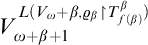 $V_{\omega +\beta +1}^{L(V_\omega +\beta ,\varrho _\beta \restriction T^\beta _{f(\beta )})}$
for
$V_{\omega +\beta +1}^{L(V_\omega +\beta ,\varrho _\beta \restriction T^\beta _{f(\beta )})}$
for
 $\beta <\alpha $
.
$\beta <\alpha $
.
And we now define
 $$ \begin{align} V_{\omega+\alpha+1}=& \bigcup_{\xi<\omega_{\alpha+1}} V_{\omega+\alpha+1}^{L(V_{\omega+\alpha},\overline{\varrho_{\alpha,f^\alpha_\xi}})}, \end{align} $$
 $$ \begin{align} \varrho_{\alpha+1}=& \left\langle V_{\omega+\alpha+1}^{L(V_{\omega+\alpha+1},\varrho_{\alpha,f^\alpha_\xi})}\mathrel{}\middle|\mathrel{}\xi<\omega_{\alpha+1}\right\rangle. \end{align} $$
Finally,
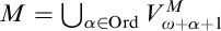 $M=\bigcup _{\alpha \in \mathrm {Ord}} V_{\omega +\alpha +1}^M$
. The handwritten notes passed on to us by some of the members of the Bristol group indicate that the original line of thought was about
$M=\bigcup _{\alpha \in \mathrm {Ord}} V_{\omega +\alpha +1}^M$
. The handwritten notes passed on to us by some of the members of the Bristol group indicate that the original line of thought was about
 $\mathbb R^M$
and
$\mathbb R^M$
and
 $\mathcal {P}(\mathbb R)^M$
, rather than
$\mathcal {P}(\mathbb R)^M$
, rather than
 $V_{\omega +1}$
and
$V_{\omega +1}$
and
 $V_{\omega +2}$
. The arguments, moreover, as to why
$V_{\omega +2}$
. The arguments, moreover, as to why
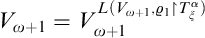 $V_{\omega +1}=V_{\omega +1}^{L(V_{\omega +1},\varrho _1\restriction T^\alpha _\xi )}$
, i.e., why no reals are added when defining
$V_{\omega +1}=V_{\omega +1}^{L(V_{\omega +1},\varrho _1\restriction T^\alpha _\xi )}$
, i.e., why no reals are added when defining
 $\mathcal {P}(\mathbb R)^M$
, was not written down in these notes. Instead it merely suggests “condensation”.
$\mathcal {P}(\mathbb R)^M$
, was not written down in these notes. Instead it merely suggests “condensation”.
While restoring the original arguments is certainly beyond us, these would be equivalent, more or less, to the arguments we presented at the first step of Section 3.
4.2 Cause
In here we will define the Bristol model in tandem: define a symmetric extension, find it a generic in
 $L[c]$
, define a symmetric extension again, repeat ad ordinalum.
$L[c]$
, define a symmetric extension again, repeat ad ordinalum.
This definition was used in [Reference Karagila8], and you can very clearly see that this is the definition that we have in mind, as it very much dominates the approach given in Section 3. As such, we really have done all the work ahead of time.
We define
 $M_\alpha ,\varrho _\alpha $
as in the decoding apparatus, i.e., as the generic objects for the symmetric iteration. We now define
$M_\alpha ,\varrho _\alpha $
as in the decoding apparatus, i.e., as the generic objects for the symmetric iteration. We now define
 $$\begin{align*}M = \bigcup _{\alpha \in \mathrm {Ord}}M_\alpha =\bigcup _{\alpha \in \mathrm {Ord}}V_{\omega +\alpha }^{M_{\alpha +1}}.\end{align*}$$
4.3 Accident
In here we will first define a class-forcing, and then argue that we can just happen to find symmetrically generic filters in
 $L[c]$
.
$L[c]$
.
Despite being the guiding view on the construction of the Bristol model, the actual argument for
 $M\models \mathsf {ZF}$
in [Reference Karagila8] is the one rising from this approach, as it is less “ad-hoc” and more structural and general. This is also the reason why the proof of the distributivity of successor steps in the original paper was proved directly, rather than the approach used in this article, which is more in line with “Cause”.
$M\models \mathsf {ZF}$
in [Reference Karagila8] is the one rising from this approach, as it is less “ad-hoc” and more structural and general. This is also the reason why the proof of the distributivity of successor steps in the original paper was proved directly, rather than the approach used in this article, which is more in line with “Cause”.
We first define the iteration. Let ![]() and
and
 ${\mathbb {Q}}_0=\operatorname {\mathrm {Add}}(\omega ,1)$
,
${\mathbb {Q}}_0=\operatorname {\mathrm {Add}}(\omega ,1)$
,
 ${\mathscr {G}}_0$
and
${\mathscr {G}}_0$
and
 ${\mathscr {F}}_0$
are the derived group and filter. Finally,
${\mathscr {F}}_0$
are the derived group and filter. Finally,
 $\dot \varrho _0$
is the canonical name for the Cohen real.
$\dot \varrho _0$
is the canonical name for the Cohen real.
Suppose that
 ${\mathbb {P}}_\alpha $
is the finite support iteration of the symmetric extensions defined so far. In the case where
${\mathbb {P}}_\alpha $
is the finite support iteration of the symmetric extensions defined so far. In the case where
 $\alpha =\beta +1$
, we define
$\alpha =\beta +1$
, we define
 $\dot {\mathbb {Q}}_\alpha $
as the name
$\dot {\mathbb {Q}}_\alpha $
as the name
 $$\begin{align*}\left\{{\textstyle\int_{\vec\pi}}\left\langle\dot V_{\omega+\alpha}^{V[\varrho_\beta\restriction A^\beta_\xi]}\mathrel{}\middle|\mathrel{}\xi\in I\right\rangle^{\bullet}\mathrel{}\middle|\mathrel{}{\textstyle\int_{\vec\pi}}\in\mathcal G_\alpha, I\in[\omega_\alpha]^{<\omega_\alpha}\right\}^{\bullet}.\end{align*}$$
Where
 $\dot V_{\omega +\alpha }^{V[x]}$
denotes the name of the rank initial segment of the extension of
$\dot V_{\omega +\alpha }^{V[x]}$
denotes the name of the rank initial segment of the extension of
 $\mathsf {IS}_\beta $
by the set x. We then define
$\mathsf {IS}_\beta $
by the set x. We then define
 $\dot \varrho _\alpha $
as the name for the generic of
$\dot \varrho _\alpha $
as the name for the generic of
 $\dot {\mathbb {Q}}_\alpha $
.
$\dot {\mathbb {Q}}_\alpha $
.
If
 $\alpha $
is a limit ordinal, we define
$\alpha $
is a limit ordinal, we define
 ${\mathbb {P}}_\alpha $
as the finite support iteration. We next define
${\mathbb {P}}_\alpha $
as the finite support iteration. We next define
 $\dot {\mathbb {Q}}_\alpha $
in the same spirit. For
$\dot {\mathbb {Q}}_\alpha $
in the same spirit. For
 $f\in \prod \operatorname {\mathrm {SC}}(\omega _{\alpha +1})$
we define
$f\in \prod \operatorname {\mathrm {SC}}(\omega _{\alpha +1})$
we define
 $$\begin{align*}\dot{\mathbb{Q}}_{\alpha,f}=\{{\textstyle\int_{\vec\pi}}\langle\dot\varrho_{\beta+1}(f(\beta+1))\mid\beta\in A\rangle\mid{\textstyle\int_{\vec\pi}}\in\mathcal G_\alpha, \sup A<\alpha\}^\bullet,\end{align*}$$
and we then define
 $\dot {\mathbb {Q}}_\alpha $
by adding the additional dimension of a bounded subset of
$\dot {\mathbb {Q}}_\alpha $
by adding the additional dimension of a bounded subset of
 $\prod \operatorname {\mathrm {SC}}(\omega _\alpha )$
. As before,
$\prod \operatorname {\mathrm {SC}}(\omega _\alpha )$
. As before,
 ${\mathscr {G}}_\alpha $
and
${\mathscr {G}}_\alpha $
and
 ${\mathscr {F}}_\alpha $
are the derived group and filter. Finally,
${\mathscr {F}}_\alpha $
are the derived group and filter. Finally,
 $\dot \varrho _\alpha $
is the name of the generic filter. Moving on, the definition of
$\dot \varrho _\alpha $
is the name of the generic filter. Moving on, the definition of
 $\dot {\mathbb {Q}}_{\alpha +1}$
and
$\dot {\mathbb {Q}}_{\alpha +1}$
and
 $\dot \varrho _{\alpha +1}$
is in line with what we have done so far.
$\dot \varrho _{\alpha +1}$
is in line with what we have done so far.
The properties of the decoding apparatus imply the distributivity of each iterand. We need to be a bit more careful here, as we are not allowed to argue in
 $L[c]$
, instead we carry on a recursive hypothesis that for successor steps
$L[c]$
, instead we carry on a recursive hypothesis that for successor steps
 ${\mathbb {P}}_\alpha $
satisfies a chain condition that allows us to prove that
${\mathbb {P}}_\alpha $
satisfies a chain condition that allows us to prove that
 $\dot {\mathbb {Q}}_\alpha $
will be isomorphic to
$\dot {\mathbb {Q}}_\alpha $
will be isomorphic to
 $\operatorname {\mathrm {Add}}(\omega _\alpha ,1)^L$
.
$\operatorname {\mathrm {Add}}(\omega _\alpha ,1)^L$
.
The conditions of Theorem 2.8 are therefore satisfied. This implies that if G is any symmetrically L-generic for
 ${\mathbb {P}}$
, the class-length iteration, then
${\mathbb {P}}$
, the class-length iteration, then
 $\mathsf {IS}^G\models \mathsf {ZF}$
, at the very least.
$\mathsf {IS}^G\models \mathsf {ZF}$
, at the very least.
By recursion we can now show that each
 $\dot \varrho _\alpha $
has a symmetric interpretation inside
$\dot \varrho _\alpha $
has a symmetric interpretation inside
 $L[c]$
, and therefore we may find an interpretation of the model which is intermediate between L and
$L[c]$
, and therefore we may find an interpretation of the model which is intermediate between L and
 $L[c]$
.
$L[c]$
.
4.4 The basic properties of the Bristol model
Proposition 4.1.
 $M\models \mathsf {ZF}$
.
$M\models \mathsf {ZF}$
.
Proof We have two slightly different proofs here, the first we mentioned in the “Accident” approach, utilising Theorem 2.8.Footnote 30 The second approach works well for “Nature” and “Cause”.
Since M is very clearly a transitive subclass of
 $L[c]$
that contains all the ordinals, it is enough to verify that it is closed under Gödel operations and that it is almost universal to conclude that it is a model of
$L[c]$
that contains all the ordinals, it is enough to verify that it is closed under Gödel operations and that it is almost universal to conclude that it is a model of
 $\mathsf {ZF}$
. The first part is easy: if
$\mathsf {ZF}$
. The first part is easy: if
 $x,y\in M$
, there is some
$x,y\in M$
, there is some
 $M_\alpha $
, or some large enough
$M_\alpha $
, or some large enough
 $V_{\omega +\alpha }$
in the “Nature” approach, such that
$V_{\omega +\alpha }$
in the “Nature” approach, such that
 $x,y\in M_\alpha $
and therefore
$x,y\in M_\alpha $
and therefore
 $\{x,y\}$
,
$\{x,y\}$
,
 $x\times y$
, etc. are all in
$x\times y$
, etc. are all in
 $M_\alpha $
and therefore in M.
$M_\alpha $
and therefore in M.
The second part is the fact mentioned at the end of “Nature” about condensation; or in the case of “Cause” this follows from the fact that for each
 $\alpha $
,
$\alpha $
,
 $V_{\omega +\alpha }^{M_\alpha }=V_{\omega +\alpha }^{M_\beta }$
for all
$V_{\omega +\alpha }^{M_\alpha }=V_{\omega +\alpha }^{M_\beta }$
for all
 $\alpha \leq \beta $
, and therefore the model is almost universal.
$\alpha \leq \beta $
, and therefore the model is almost universal.
Proposition 4.2.
 $M\models \forall x(V\neq L(x))$
.
$M\models \forall x(V\neq L(x))$
.
Proof If
 $x\in M$
, then there is some
$x\in M$
, then there is some
 $\alpha $
such that
$\alpha $
such that
 $x\in M_\alpha $
, and therefore
$x\in M_\alpha $
, and therefore
 $L(x)\subseteq M_\alpha $
. But since
$L(x)\subseteq M_\alpha $
. But since
 $M_\alpha \subsetneq M_{\alpha +1}\subseteq M$
, we have that
$M_\alpha \subsetneq M_{\alpha +1}\subseteq M$
, we have that
 $L(x)\neq M$
. In the “Nature” approach we need to be slightly more careful, as we have to verify that if
$L(x)\neq M$
. In the “Nature” approach we need to be slightly more careful, as we have to verify that if
 $x\in V_\alpha $
, then
$x\in V_\alpha $
, then
 $V_{\alpha +1}\notin L(x)$
. One way of doing this would be to argue that
$V_{\alpha +1}\notin L(x)$
. One way of doing this would be to argue that
 $\varrho _\alpha \restriction A^\alpha _\xi $
are all generic over
$\varrho _\alpha \restriction A^\alpha _\xi $
are all generic over
 $L(V_\alpha )$
, and therefore cannot be elements of this model.
$L(V_\alpha )$
, and therefore cannot be elements of this model.
We will see other ways of deducing Proposition 4.2 later on, in ways that will be significantly more informative and more general.
5 Errata to “the Abyss”
Here we correct some minor gaps and mistakes in the original paper. These mistakes repeat, once with the cases of
 $\alpha =0$
and
$\alpha =0$
and
 $\alpha =\beta +2$
, and once with the cases of
$\alpha =\beta +2$
, and once with the cases of
 $\alpha =\omega $
and a general limit ordinal.
$\alpha =\omega $
and a general limit ordinal.
We repeat the remark we made in footnote 28: in [Reference Karagila8] the proof of Lemma 4.7, dealing with the genericity of
 $\varrho _\omega $
, contains a typo, whereas
$\varrho _\omega $
, contains a typo, whereas
 $B_n$
is defined as
$B_n$
is defined as
 $\bigcup \mathcal B_n$
, and it should have been defined as
$\bigcup \mathcal B_n$
, and it should have been defined as
 $\operatorname {\mathrm {dom}}\mathcal B_{n-1}$
. This is somewhat inconsequential, as the more general proof where
$\operatorname {\mathrm {dom}}\mathcal B_{n-1}$
. This is somewhat inconsequential, as the more general proof where
 $\alpha $
is a limit, in Lemma 4.20, is written correctly.
$\alpha $
is a limit, in Lemma 4.20, is written correctly.
We also point out that there is a minor mistake in the construction’s induction hypothesis, where the requirement that
 ${\mathbb {P}}_\alpha $
satisfies the
${\mathbb {P}}_\alpha $
satisfies the
 $\aleph _\alpha $
-c.c. will not hold for limit ordinals, only for
$\aleph _\alpha $
-c.c. will not hold for limit ordinals, only for
 $0$
and successor ordinals. We can modify this by defining a notion of “symmetric chain condition”,Footnote
31
but this is an unnecessary complication. We simply do not use the chain condition assumption for limit iterands.
$0$
and successor ordinals. We can modify this by defining a notion of “symmetric chain condition”,Footnote
31
but this is an unnecessary complication. We simply do not use the chain condition assumption for limit iterands.
5.1 Corrections to Lemma 2.12/4.1
Lemma 2.12 is read in the context of the first steps. Namely,
 ${\mathbb {P}}$
is Cohen forcing,
${\mathbb {P}}$
is Cohen forcing,
 $\dot {\mathbb {Q}}$
is the name of the forcing adding
$\dot {\mathbb {Q}}$
is the name of the forcing adding
 $\varrho _1$
, denoted in that lemma by
$\varrho _1$
, denoted in that lemma by
 $\sigma $
. As such
$\sigma $
. As such
 ${\mathsf {HS}}$
is the class of hereditarily symmetric names defined in the very first step.
${\mathsf {HS}}$
is the class of hereditarily symmetric names defined in the very first step.
Lemma [Reference Karagila8, Lemma 2.12].
Suppose that
 $\dot D\in {\mathsf {HS}}$
and
$\dot D\in {\mathsf {HS}}$
and
 $p\mathrel {\Vdash }\dot D\subseteq \dot {\mathbb {Q}}$
is a dense open set. There is some
$p\mathrel {\Vdash }\dot D\subseteq \dot {\mathbb {Q}}$
is a dense open set. There is some
 $\eta <\omega _1$
such that for every
$\eta <\omega _1$
such that for every
 $\pi $
and A such that
$\pi $
and A such that
 ${p\mathrel {\Vdash }\pi \dot \sigma _A\in \dot D}$
and
${p\mathrel {\Vdash }\pi \dot \sigma _A\in \dot D}$
and
 $\eta \subseteq A$
, if
$\eta \subseteq A$
, if
 $\tau \dot \sigma _A$
is a condition such that
$\tau \dot \sigma _A$
is a condition such that
 $p\mathrel {\Vdash }\pi \dot \sigma _\eta =\tau \dot \sigma _\eta $
, then
$p\mathrel {\Vdash }\pi \dot \sigma _\eta =\tau \dot \sigma _\eta $
, then
 $p\mathrel {\Vdash }\tau \dot \sigma _A\in \dot D$
as well.
$p\mathrel {\Vdash }\tau \dot \sigma _A\in \dot D$
as well.
In the article this lemma was used twice. The first consequence is the genericity of
 $\varrho _1$
,Footnote
32
and the second is to show that
$\varrho _1$
,Footnote
32
and the second is to show that
 $\dot {\mathbb {Q}}$
is
$\dot {\mathbb {Q}}$
is
 $\sigma $
-distributive. The proof is very similar to the proof of Proposition 3.10. Nevertheless, when we have two permutations
$\sigma $
-distributive. The proof is very similar to the proof of Proposition 3.10. Nevertheless, when we have two permutations
 $\pi $
and
$\pi $
and
 $\tau $
, we want to move
$\tau $
, we want to move
 $\tau $
so that it agrees with
$\tau $
so that it agrees with
 $\pi $
.
$\pi $
.
For this we need not only that
 $\iota (\tau )\restriction A=\iota (\pi )\restriction A$
, but also that their inverses agree on A. In the case of the genericity of
$\iota (\tau )\restriction A=\iota (\pi )\restriction A$
, but also that their inverses agree on A. In the case of the genericity of
 $\varrho _1$
we take
$\varrho _1$
we take
 $\pi =\operatorname {\mathrm {id}}$
, in which case this property holds trivially. Indeed, this is the very strategy of the proof of Proposition 3.10.
$\pi =\operatorname {\mathrm {id}}$
, in which case this property holds trivially. Indeed, this is the very strategy of the proof of Proposition 3.10.
To prove that
 $\dot {\mathbb {Q}}$
is
$\dot {\mathbb {Q}}$
is
 $\sigma $
-distributive we interpret the lemma above as saying that for a condition
$\sigma $
-distributive we interpret the lemma above as saying that for a condition
 $p\in {\mathbb {P}}$
, there is an ordinal
$p\in {\mathbb {P}}$
, there is an ordinal
 $\eta $
, such that deciding whether a condition from
$\eta $
, such that deciding whether a condition from
 $\dot {\mathbb {Q}}$
, whose domain is at least
$\dot {\mathbb {Q}}$
, whose domain is at least
 $\eta $
, lies in
$\eta $
, lies in
 $\dot D$
depends only on the permutation
$\dot D$
depends only on the permutation
 $\pi $
. We then utilise the fact
$\pi $
. We then utilise the fact
 ${\mathbb {P}}$
is c.c.c. to show that this
${\mathbb {P}}$
is c.c.c. to show that this
 $\eta $
can be bound uniformly depending on
$\eta $
can be bound uniformly depending on
 $\dot D$
. Now, if
$\dot D$
. Now, if
 $\dot D_n$
are names for a sequence of dense open sets, we can uniformly bound all of them by some
$\dot D_n$
are names for a sequence of dense open sets, we can uniformly bound all of them by some
 $\eta $
. Now if we take any condition whose domain is at least this
$\eta $
. Now if we take any condition whose domain is at least this
 $\eta $
, we may extend it into each
$\eta $
, we may extend it into each
 $\dot D_n$
, but this means that such extension lies, in fact, in all the
$\dot D_n$
, but this means that such extension lies, in fact, in all the
 $\dot D_n$
simultaneously, and therefore the intersection is also dense.
$\dot D_n$
simultaneously, and therefore the intersection is also dense.
Once we add the condition that
 $\iota (\pi )^{-1}\restriction A=\iota (\tau )^{-1}\restriction A$
, the proof as written in [Reference Karagila8] follows through. Alternatively, and perhaps more wisely, for proving the distributivity one should rely on the absoluteness proof that we used in this manuscript, which is also mentioned in the “Abyss”.
$\iota (\pi )^{-1}\restriction A=\iota (\tau )^{-1}\restriction A$
, the proof as written in [Reference Karagila8] follows through. Alternatively, and perhaps more wisely, for proving the distributivity one should rely on the absoluteness proof that we used in this manuscript, which is also mentioned in the “Abyss”.
Lemma 4.1 is precisely the same, in the context of successor iterations. There is no need to repeat that which has been said.
5.2 Corrections to Proposition 4.4/4.15
These two propositions are dealing with limit iterations. They show that
 $\langle \varrho _\beta \mid \beta <\alpha \rangle $
is symmetrically generic for
$\langle \varrho _\beta \mid \beta <\alpha \rangle $
is symmetrically generic for
 ${\mathbb {P}}_\alpha $
, with Proposition 4.4 dealing with the case
${\mathbb {P}}_\alpha $
, with Proposition 4.4 dealing with the case
 $\alpha =\omega $
, which was treated separately in the article.
$\alpha =\omega $
, which was treated separately in the article.
Proposition [Reference Karagila8, Proposition 4.4].
Suppose that
 $D\subseteq {\mathbb {P}}_\omega $
is a symmetrically dense open set, then there are
$D\subseteq {\mathbb {P}}_\omega $
is a symmetrically dense open set, then there are
 $\langle \beta _n\mid n<\omega \rangle $
such that
$\langle \beta _n\mid n<\omega \rangle $
such that
 $\langle \dot \varrho _n\restriction \beta _n\mid n<\omega \rangle \in D$
.
$\langle \dot \varrho _n\restriction \beta _n\mid n<\omega \rangle \in D$
.
In the article the proof takes a symmetrically dense open set D, and an excellent support
 $\vec H$
witnessing that. We then generate some sequence of domains such that when we extend the condition
$\vec H$
witnessing that. We then generate some sequence of domains such that when we extend the condition
 $\langle \varrho _\beta \restriction X_\beta \mid \beta <\alpha \rangle $
into D, then we can “correct” it using automorphisms which lie in
$\langle \varrho _\beta \restriction X_\beta \mid \beta <\alpha \rangle $
into D, then we can “correct” it using automorphisms which lie in
 $\vec H$
. Namely, each coordinate of
$\vec H$
. Namely, each coordinate of
 $\vec H$
is of the form
$\vec H$
is of the form
 $\operatorname {\mathrm {fix}}(\mathcal B_\beta )$
, and we take
$\operatorname {\mathrm {fix}}(\mathcal B_\beta )$
, and we take
 $X_\beta $
to be
$X_\beta $
to be
 $\sup \operatorname {\mathrm {dom}}\mathcal B_\beta +1$
, and therefore our starting condition is
$\sup \operatorname {\mathrm {dom}}\mathcal B_\beta +1$
, and therefore our starting condition is
 $\langle \varrho _\beta \restriction X_\beta \mid \beta <\alpha \rangle $
.
$\langle \varrho _\beta \restriction X_\beta \mid \beta <\alpha \rangle $
.
The idea is fine, and it is somehow intuitively clear what should happen. However the proof described above, taken from the “Abyss”, will not work. The first hint is obvious:
 $\varrho _\beta $
has domain
$\varrho _\beta $
has domain
 $\omega _\beta $
, and
$\omega _\beta $
, and
 $X_\beta $
is a bounded subset of
$X_\beta $
is a bounded subset of
 $\omega _{\beta +1}$
. We can resolve this issue by considering
$\omega _{\beta +1}$
. We can resolve this issue by considering
 $\varrho _{\beta +1}\restriction X_\beta $
, but this raises the obvious question, what should we do with limit steps and with
$\varrho _{\beta +1}\restriction X_\beta $
, but this raises the obvious question, what should we do with limit steps and with
 $\varrho _0$
?
$\varrho _0$
?
Let us prove this proposition in its general form.
Proposition 5.1 [Reference Karagila8, Proposition 4.15].
Let
 $\alpha $
be a limit ordinal, then the sequence
$\alpha $
be a limit ordinal, then the sequence
 $\langle \varrho _\beta \mid \beta <\alpha \rangle $
is symmetrically L-generic for
$\langle \varrho _\beta \mid \beta <\alpha \rangle $
is symmetrically L-generic for
 ${\mathbb {P}}_\alpha $
.
${\mathbb {P}}_\alpha $
.
Proof Let D be a symmetrically dense open set. Our goal is to find a condition of the form
 $\langle \varrho _\beta \restriction X_\beta \mid \beta <\alpha \rangle $
, for appropriate
$\langle \varrho _\beta \restriction X_\beta \mid \beta <\alpha \rangle $
, for appropriate
 $X_\beta $
, in D.
$X_\beta $
, in D.
Let
 $\vec H$
denote the excellent support witnessing that D is a symmetrically dense open set. For
$\vec H$
denote the excellent support witnessing that D is a symmetrically dense open set. For
 $\beta <\alpha $
let
$\beta <\alpha $
let
 $\xi _{\beta +1}$
the ordinal defined by either,
$\xi _{\beta +1}$
the ordinal defined by either,
-
(1) when
$\beta $
is
$0$
or a successor let
$\mathcal B_\beta $
be such that
$H_\beta =\operatorname {\mathrm {fix}}(\mathcal B_\beta )$
, and define
$\xi _{\beta +1}=\sup \operatorname {\mathrm {dom}}\mathcal B_\beta $
; -
(2) when
$\beta $
is a limit let
$\xi _{\beta +1}$
be an ordinal
$\xi $
such that for some
$f \text{ in} \prod \operatorname {\mathrm {SC}}(\omega _\beta )$
,
$H_\beta =K_{\xi ,f_\beta }$
; -
(3) when
$H_\beta ={\mathscr {G}}_\beta $
, set
$\xi _{\beta +1}=0$
.


For a limit ordinal
 $\beta $
, let
$\beta $
, let
 $E_\beta \subseteq \prod \operatorname {\mathrm {SC}}(\omega _\beta )$
be defined by
$E_\beta \subseteq \prod \operatorname {\mathrm {SC}}(\omega _\beta )$
be defined by
 $\prod _{\gamma <\beta }(\xi _{\gamma +1}+1)$
, and let
$\prod _{\gamma <\beta }(\xi _{\gamma +1}+1)$
, and let
 $A_\beta $
denote
$A_\beta $
denote
 $\sup \{\gamma <\beta \mid H_{\gamma +1}\neq {\mathscr {G}}_{\gamma +1}\}$
; if
$\sup \{\gamma <\beta \mid H_{\gamma +1}\neq {\mathscr {G}}_{\gamma +1}\}$
; if
 $\beta $
is a limit ordinal such that
$\beta $
is a limit ordinal such that
 $H_\gamma ={\mathscr {G}}_\gamma $
for all
$H_\gamma ={\mathscr {G}}_\gamma $
for all
 $\gamma \geq \beta $
, set
$\gamma \geq \beta $
, set
 $E_\beta =A_\beta =\varnothing $
. Now define
$E_\beta =A_\beta =\varnothing $
. Now define
 $Y_\beta $
as
$Y_\beta $
as
 $0$
for
$0$
for
 $\beta =0$
,
$\beta =0$
,
 $\xi _\beta $
for successors, and
$\xi _\beta $
for successors, and
 $(E_\beta ,A_\beta )$
for limit ordinals.
$(E_\beta ,A_\beta )$
for limit ordinals.
The goal is to find the “domain” over which
 $\vec H$
must be the identity, and use that to start our journey into D. Let p be the condition
$\vec H$
must be the identity, and use that to start our journey into D. Let p be the condition
 $\langle \varrho _\beta \restriction Y_\beta \mid \beta <\alpha \rangle $
. By its very definition, p is not moved by any
$\langle \varrho _\beta \restriction Y_\beta \mid \beta <\alpha \rangle $
. By its very definition, p is not moved by any
 $\vec \pi \in \vec H$
. Using the density of D we can now extend p to a condition
$\vec \pi \in \vec H$
. Using the density of D we can now extend p to a condition
 $p_0\in D$
. Moreover, since D is in L, we may assume that the first coordinate of
$p_0\in D$
. Moreover, since D is in L, we may assume that the first coordinate of
 $p_0$
agrees with
$p_0$
agrees with
 $\varrho _0$
, i.e., the Cohen real c, and by shrinking
$\varrho _0$
, i.e., the Cohen real c, and by shrinking
 $H_0$
if necessary, we may assume that
$H_0$
if necessary, we may assume that
 $p_0(0)$
is not moved by automorphisms in
$p_0(0)$
is not moved by automorphisms in
 $H_0$
.
$H_0$
.
If
 $p_0$
is not compatible with
$p_0$
is not compatible with
 $\langle \varrho _\beta \mid \beta <\alpha \rangle $
, let
$\langle \varrho _\beta \mid \beta <\alpha \rangle $
, let
 $\beta $
be the least coordinate witnessing that. By the choice of
$\beta $
be the least coordinate witnessing that. By the choice of
 $Y_\beta $
we can find
$Y_\beta $
we can find
 $\vec \pi \in H\restriction \beta $
, and if
$\vec \pi \in H\restriction \beta $
, and if
 $\beta $
is not a limit ordinal then we may assume
$\beta $
is not a limit ordinal then we may assume
 $\vec \pi $
has a single non-trivial coordinate too, such that by taking
$\vec \pi $
has a single non-trivial coordinate too, such that by taking
 $p_1={\textstyle \int _{\vec \pi }}p_0$
, the following hold:
$p_1={\textstyle \int _{\vec \pi }}p_0$
, the following hold:
-
(1)
$\operatorname {\mathrm {supp}}(p_0)=\operatorname {\mathrm {supp}}(p_1)$
; -
(2)
$p_0\restriction \beta =p_1\restriction \beta $
; -
(3)
$p_1(\beta )$
is indeed compatible with
$\varrho _\beta $
.


The reason we can do that is exactly upwards homogeneity combined with our choice of p, which
 $p_0$
extended. As we did not increase the non-trivial coordinates when moving from
$p_0$
extended. As we did not increase the non-trivial coordinates when moving from
 $p_0$
to
$p_0$
to
 $p_1$
, we may proceed by recursion and after finitely many steps the process must halt with some
$p_1$
, we may proceed by recursion and after finitely many steps the process must halt with some
 $p_n\in D$
.
$p_n\in D$
.
Indeed, the main point is the fact that we may assume that the first coordinate, for which true genericity is already assumed, is compatible with the Cohen real, and then we can modify any further coordinates recursively using upward homogeneity, combined with the fact that we only need to change things outside of the domains we found, which means that the needed automorphisms can be found in
 $\vec H$
.
$\vec H$
.
6 Removing the constructibility assumptions
Now that we have constructed the Bristol model, and we have a good idea about how the construction works, we can ask the obvious question: do we really need
 $V=L$
in the ground model? The answer, of course, is not really.
$V=L$
in the ground model? The answer, of course, is not really.
We have merely used three assumptions:
 $\mathsf {GCH}$
,
$\mathsf {GCH}$
,
 $\square ^*_\lambda $
for singular
$\square ^*_\lambda $
for singular
 $\lambda $
, and global choice for fixing the Bristol sequence. Of those three, the last one can be easily dispensed, and we will discuss this in Section 7. So we are left with only two assumptions which are compatible with a large range of models, including all known inner models from large cardinals below a subcompact.
$\lambda $
, and global choice for fixing the Bristol sequence. Of those three, the last one can be easily dispensed, and we will discuss this in Section 7. So we are left with only two assumptions which are compatible with a large range of models, including all known inner models from large cardinals below a subcompact.
This raises an interesting question, of course. What kind of large cardinals can the Bristol model accommodate, assuming they existed in the ground model?
Proposition 6.1. If A is a set of ordinals in the Bristol model, then there is a real number r such that
 $A\in V[r]$
, and moreover
$A\in V[r]$
, and moreover
 $r\in V$
or r is Cohen over V.
$r\in V$
or r is Cohen over V.
Proof Note that
 $V[A]$
is a model of
$V[A]$
is a model of
 $\mathsf {ZFC}$
intermediate to V and
$\mathsf {ZFC}$
intermediate to V and
 $V[c]$
, and therefore
$V[c]$
, and therefore
 $V[A]$
is equivalent to some
$V[A]$
is equivalent to some
 $V[r]$
.
$V[r]$
.
This leads to an immediate corollary: if
 $\kappa $
is a large cardinal defined by the existence (or lack thereof) of sets of ordinals, and this largeness is preserved by adding a Cohen real, then
$\kappa $
is a large cardinal defined by the existence (or lack thereof) of sets of ordinals, and this largeness is preserved by adding a Cohen real, then
 $\kappa $
remains large in the Bristol model.
$\kappa $
remains large in the Bristol model.
For example, if
 $\kappa $
is Mahlo, then the stationary set of regular cardinals remains stationary in M, and thus
$\kappa $
is Mahlo, then the stationary set of regular cardinals remains stationary in M, and thus
 $\kappa $
remains Mahlo. If we define a weakly compact cardinal by stating that every colouring of
$\kappa $
remains Mahlo. If we define a weakly compact cardinal by stating that every colouring of
 $[\kappa ]^2$
in
$[\kappa ]^2$
in
 $2$
colours has a homogeneous subset, this too is given by sets of ordinals, and so it continues to hold in M.
$2$
colours has a homogeneous subset, this too is given by sets of ordinals, and so it continues to hold in M.
We will see in Section 9 that this can be extended from sets of ordinals to sets of sets of ordinals, and so on, as long as we iterate power sets less than
 $\kappa $
times, the largeness remains. So, for example, any measure on a ground model measurable cardinal will have a unique extension in the Bristol model. Strong cardinals, defined by extenders, are also preserved.
$\kappa $
times, the largeness remains. So, for example, any measure on a ground model measurable cardinal will have a unique extension in the Bristol model. Strong cardinals, defined by extenders, are also preserved.
6.1 Limitations
Despite this handsome accommodation of large cardinal assumptions in the ground model, as well as in the Bristol model itself, we can put a stop to this. Indeed, if
 $\kappa $
is a supercompact cardinal, then there is a notable shortage of
$\kappa $
is a supercompact cardinal, then there is a notable shortage of
 $\square ^*_\lambda $
sequences for singular
$\square ^*_\lambda $
sequences for singular
 $\lambda $
such that
$\lambda $
such that
 $\operatorname {\mathrm {cf}}(\lambda )<\kappa <\lambda $
. We may ask ourselves, perhaps we can salvage permutable scales without having
$\operatorname {\mathrm {cf}}(\lambda )<\kappa <\lambda $
. We may ask ourselves, perhaps we can salvage permutable scales without having
 $\square ^*_\lambda $
?
$\square ^*_\lambda $
?
Theorem 6.2 (The Bristol group).
Suppose that
 $\kappa $
is a supercompact cardinal and
$\kappa $
is a supercompact cardinal and
 $\lambda>\kappa >\operatorname {\mathrm {cf}}(\lambda )$
. Then there are no permutable scales on
$\lambda>\kappa >\operatorname {\mathrm {cf}}(\lambda )$
. Then there are no permutable scales on
 $\prod \operatorname {\mathrm {SC}}(\lambda )$
.
$\prod \operatorname {\mathrm {SC}}(\lambda )$
.
Recall that we are still working under the assumption of
 $\mathsf {GCH}$
. Removing it will require adding
$\mathsf {GCH}$
. Removing it will require adding
 $2^\lambda <2^{\lambda ^+}$
, which itself is a harmless assumption as it holds for all strong limit cardinals above
$2^\lambda <2^{\lambda ^+}$
, which itself is a harmless assumption as it holds for all strong limit cardinals above
 $\kappa $
.
$\kappa $
.
Proof Let
 $F=\{f_\alpha \mid \alpha <\lambda ^+\}$
be a scale in
$F=\{f_\alpha \mid \alpha <\lambda ^+\}$
be a scale in
 $\prod \operatorname {\mathrm {SC}}(\lambda )$
, and let
$\prod \operatorname {\mathrm {SC}}(\lambda )$
, and let
 $\pi $
be a permutation of
$\pi $
be a permutation of
 $\lambda ^+$
, not necessarily bounded, which is not implemented by any sequence of permutations,
$\lambda ^+$
, not necessarily bounded, which is not implemented by any sequence of permutations,
 $\vec \pi $
. Pick
$\vec \pi $
. Pick
 $j\colon V\to W$
an elementary embedding with critical point
$j\colon V\to W$
an elementary embedding with critical point
 $\kappa $
witnessing that
$\kappa $
witnessing that
 $\kappa $
is at least
$\kappa $
is at least
 $\lambda ^+$
-supercompact, so in particular
$\lambda ^+$
-supercompact, so in particular
 $j(\kappa )>\lambda ^+$
. We denote by
$j(\kappa )>\lambda ^+$
. We denote by
 $G=\{g_\alpha \mid \alpha <j(\lambda ^+)\}$
the scale
$G=\{g_\alpha \mid \alpha <j(\lambda ^+)\}$
the scale
 $j(F)$
, which is a scale in
$j(F)$
, which is a scale in
 $j(\prod \operatorname {\mathrm {SC}}(\lambda ))$
which is equal to
$j(\prod \operatorname {\mathrm {SC}}(\lambda ))$
which is equal to
 $\prod \operatorname {\mathrm {SC}}(j(\lambda ))^M$
.
$\prod \operatorname {\mathrm {SC}}(j(\lambda ))^M$
.
Let
 $\nu =\sup j"\lambda ^+$
, then
$\nu =\sup j"\lambda ^+$
, then
 $\nu $
is closed under
$\nu $
is closed under
 $j(\pi )$
, so we can let
$j(\pi )$
, so we can let
 $\tau $
denote
$\tau $
denote
 $j(\pi )\restriction \nu $
, which is a bounded permutation of
$j(\pi )\restriction \nu $
, which is a bounded permutation of
 $j(\lambda ^+)$
.
$j(\lambda ^+)$
.
Suppose that there was a sequence of permutations
 $\vec \tau $
that implemented
$\vec \tau $
that implemented
 $\tau $
, then for
$\tau $
, then for
 $\alpha <\lambda ^+$
and
$\alpha <\lambda ^+$
and
 $\mu <\lambda $
, we have
$\mu <\lambda $
, we have
 $g_{j(\alpha )}(j(\mu ^+))=j(f_\alpha (\mu ^+))$
and
$g_{j(\alpha )}(j(\mu ^+))=j(f_\alpha (\mu ^+))$
and
 $\tau (j(\alpha ))=j(\pi (\alpha ))$
. Combining this with the assumption that
$\tau (j(\alpha ))=j(\pi (\alpha ))$
. Combining this with the assumption that
 $\vec \tau $
implements
$\vec \tau $
implements
 $\tau $
, we get that
$\tau $
, we get that
 $$\begin{align*}\tau_{j(\mu^+)}(j(f_\alpha(\mu^+)))=j(f_{\pi(\alpha)}(\mu^+)).\end{align*}$$
We use this to define
 $\pi _{\mu ^+}\colon \mu ^+\to \mu ^+$
. If
$\pi _{\mu ^+}\colon \mu ^+\to \mu ^+$
. If
 $\tau _{j(\mu ^+)}(j(\xi ))=j(\zeta )$
for some
$\tau _{j(\mu ^+)}(j(\xi ))=j(\zeta )$
for some
 $\zeta $
, define
$\zeta $
, define
 $\pi _{\mu ^+}(\xi )=\zeta $
; otherwise
$\pi _{\mu ^+}(\xi )=\zeta $
; otherwise
 $\pi _{\mu ^+}(\xi )=\xi $
. This is well-defined, since
$\pi _{\mu ^+}(\xi )=\xi $
. This is well-defined, since
 $\tau _{j(\mu ^+)}$
is itself a permutation of
$\tau _{j(\mu ^+)}$
is itself a permutation of
 $j(\mu ^+)$
, and so
$j(\mu ^+)$
, and so
 $j(\zeta )<j(\mu ^+)$
. This is also a permutation by similar reasons.
$j(\zeta )<j(\mu ^+)$
. This is also a permutation by similar reasons.
Finally, we claim that
 $\vec \pi $
implements
$\vec \pi $
implements
 $\pi $
. Fix
$\pi $
. Fix
 $\alpha <\lambda ^+$
, then for any large enough
$\alpha <\lambda ^+$
, then for any large enough
 $\mu ^+<\lambda $
,
$\mu ^+<\lambda $
,
 $\tau _{j(\mu ^+)}(j(f_\alpha (\mu ^+)))=j(f_{\pi (\alpha )}(\mu ^+))$
, which means that we defined
$\tau _{j(\mu ^+)}(j(f_\alpha (\mu ^+)))=j(f_{\pi (\alpha )}(\mu ^+))$
, which means that we defined
 $\pi _{\mu ^+}$
to be exactly
$\pi _{\mu ^+}$
to be exactly
 $f_{\pi (\alpha )}(\mu ^+)$
.
$f_{\pi (\alpha )}(\mu ^+)$
.
We have shown that if F can be used to implement all bounded permutations, then it can be used to implement all permutations, but that is definitely impossible on grounds of cardinal arithmetic.
7 Gaps in the multiverse
The Bristol model, as we said at first, is a particularly striking counterexample to our understanding of intermediate models when the axiom of choice is not assumed. Working in V’s meta-theory, we can consider the collection of all intermediate models between V and
 $V[c]$
. We remarked before, those models which satisfy
$V[c]$
. We remarked before, those models which satisfy
 $\mathsf {ZFC}$
are exactly V itself or Cohen extensions of the form
$\mathsf {ZFC}$
are exactly V itself or Cohen extensions of the form
 $V[r]$
for some
$V[r]$
for some
 $r\in \mathbb R^{V[c]}$
.
$r\in \mathbb R^{V[c]}$
.
What about models of
 $\mathsf {ZF}$
? We have, of course, symmetric extensions. These were studied extensively by Grigorieff in [Reference Grigorieff3], and later by Usuba in [Reference Usuba23]. Grigorieff proved that if M is a model such that
$\mathsf {ZF}$
? We have, of course, symmetric extensions. These were studied extensively by Grigorieff in [Reference Grigorieff3], and later by Usuba in [Reference Usuba23]. Grigorieff proved that if M is a model such that
 $V\subseteq M\subseteq V[G]$
, then M is a symmetric extension given by the same forcing used to add G if and only if
$V\subseteq M\subseteq V[G]$
, then M is a symmetric extension given by the same forcing used to add G if and only if
 $M=(\mathrm {HOD}_{V\cup x})^{V[G]}$
for some set
$M=(\mathrm {HOD}_{V\cup x})^{V[G]}$
for some set
 $x\in V[G]$
. Usuba extended this and showed that in general, M is a symmetric extension of V if and only if
$x\in V[G]$
. Usuba extended this and showed that in general, M is a symmetric extension of V if and only if
 $M=V(x)$
for some set x.
$M=V(x)$
for some set x.
The construction of the Bristol model shows that there is indeed a difference between the two results. Indeed, by counting the number of possible automorphism groups and filters of groups we can see that there cannot be more than
 $\aleph _3$
distinct symmetric extensions of
$\aleph _3$
distinct symmetric extensions of
 $\operatorname {\mathrm {Add}}(\omega ,1)$
over L.Footnote
33
Yet, the construction of the Bristol model goes through a proper class of steps, and even if we did not formally prove that each separate one is of the form
$\operatorname {\mathrm {Add}}(\omega ,1)$
over L.Footnote
33
Yet, the construction of the Bristol model goes through a proper class of steps, and even if we did not formally prove that each separate one is of the form
 $L(x)$
, we may take
$L(x)$
, we may take
 $L(V_\alpha ^M)$
as our models. By Usuba’s result, these are all symmetric extensions of L, but of course most of them are not symmetric extensions where the forcing used is the Cohen forcing.
$L(V_\alpha ^M)$
as our models. By Usuba’s result, these are all symmetric extensions of L, but of course most of them are not symmetric extensions where the forcing used is the Cohen forcing.
So when we consider the multiverse of symmetric extensions of L, even those that are landlocked inside
 $L[c]$
, we seem to have two different options. But we want to study all intermediate models, and these include the Bristol model, which is very much not a symmetric extension of L, by any means, as Usuba’s result indicates. So what can we say about the multiverse of
$L[c]$
, we seem to have two different options. But we want to study all intermediate models, and these include the Bristol model, which is very much not a symmetric extension of L, by any means, as Usuba’s result indicates. So what can we say about the multiverse of
 $\mathsf {ZF}$
models?
$\mathsf {ZF}$
models?
First, let us ask, how many Bristol models are there? Of course, there is the canonical one, given by the
 $<_L$
-minimal Bristol sequence. But there are certainly more. Simply by removing some of the sets or functions in any given point in the Bristol sequence we invariably create a new Bristol model.
$<_L$
-minimal Bristol sequence. But there are certainly more. Simply by removing some of the sets or functions in any given point in the Bristol sequence we invariably create a new Bristol model.
Proposition 7.1. Assuming
 $\mathsf {GCH}$
and that
$\mathsf {GCH}$
and that
 $\square ^*_\lambda $
holds for all singular
$\square ^*_\lambda $
holds for all singular
 $\lambda $
, there is a class forcing which does not add sets whose generic is a Bristol sequence.
$\lambda $
, there is a class forcing which does not add sets whose generic is a Bristol sequence.
This is done, of course, by approximating the Bristol sequence with set-length initial segments. This is also the way we can remove global choice from the assumptions. Indeed, if V was a model of
 $\mathsf {ZFC}$
, add a generic Bristol sequence, use it to define a Bristol model between V and
$\mathsf {ZFC}$
, add a generic Bristol sequence, use it to define a Bristol model between V and
 $V[c]$
, where c is a Cohen real, and promptly forget about this generic sequence.
$V[c]$
, where c is a Cohen real, and promptly forget about this generic sequence.
As very clearly the Bristol model is definable from its Bristol sequence in
 $V[c]$
, this means that there may be undefinable Bristol models. And indeed, this can very much be the case.
$V[c]$
, this means that there may be undefinable Bristol models. And indeed, this can very much be the case.
Theorem 7.2. Suppose that V is a countable transitive model of
 $\mathsf {ZFC}+\mathsf {GCH}+\square ^*_\lambda $
for all singular cardinals
$\mathsf {ZFC}+\mathsf {GCH}+\square ^*_\lambda $
for all singular cardinals
 $\lambda $
, and let c be a Cohen real over V. Then there are uncountably many Bristol models intermediate between V and
$\lambda $
, and let c be a Cohen real over V. Then there are uncountably many Bristol models intermediate between V and
 $V[c]$
.
$V[c]$
.
Proof Given two Bristol sequences such that
 $\mathcal A_0$
and
$\mathcal A_0$
and
 $\mathcal A^{\prime }_0$
are the two permutable families on
$\mathcal A^{\prime }_0$
are the two permutable families on
 $\omega $
and such that
$\omega $
and such that
 $\bigcup \mathcal A_0\cap \bigcup \mathcal A_0'$
is finite, the two Bristol models are distinct. This can be easily arranged, for example, taking
$\bigcup \mathcal A_0\cap \bigcup \mathcal A_0'$
is finite, the two Bristol models are distinct. This can be easily arranged, for example, taking
 $\mathcal A_0$
to only have subsets of even integers and
$\mathcal A_0$
to only have subsets of even integers and
 $\mathcal A^{\prime }_0$
only has subsets of odd integers. This can be extended to any other step in the Bristol sequence. We can now easily construct uncountably many distinct Bristol models by simply considering with each subset of
$\mathcal A^{\prime }_0$
only has subsets of odd integers. This can be extended to any other step in the Bristol sequence. We can now easily construct uncountably many distinct Bristol models by simply considering with each subset of
 $\mathrm {Ord}^V$
how to modify a given, or indeed a generic, Bristol sequence.
$\mathrm {Ord}^V$
how to modify a given, or indeed a generic, Bristol sequence.
This is in stark contrast to the case of intermediate models of
 $\mathsf {ZFC}$
of which there are only not just countably many, but there is a set of all the necessary generators in
$\mathsf {ZFC}$
of which there are only not just countably many, but there is a set of all the necessary generators in
 $V[c]$
, and the same can be said about symmetric extensions given by the Cohen forcing itself, as Grigorieff’s theorem shows. And while there is a proper class of symmetric extensions of V, it is still enumerated by the sets in
$V[c]$
, and the same can be said about symmetric extensions given by the Cohen forcing itself, as Grigorieff’s theorem shows. And while there is a proper class of symmetric extensions of V, it is still enumerated by the sets in
 $V[c]$
, making it countable in the meta-theory.
$V[c]$
, making it countable in the meta-theory.
Therefore between V and
 $V[c]$
most models are models of
$V[c]$
most models are models of
 $\mathsf {ZF}$
, they are not symmetric extensions of V, and in fact they are not definable in
$\mathsf {ZF}$
, they are not symmetric extensions of V, and in fact they are not definable in
 $V[c]$
. To make matters worse, inside each Bristol model, we can find a different real, and use that real to interpret the Bristol sequence. Just as well, we may also use one of the
$V[c]$
. To make matters worse, inside each Bristol model, we can find a different real, and use that real to interpret the Bristol sequence. Just as well, we may also use one of the
 $\varrho _{\alpha +1}\restriction A^\alpha _\xi $
to interpret the Bristol model construction above a certain stage.
$\varrho _{\alpha +1}\restriction A^\alpha _\xi $
to interpret the Bristol model construction above a certain stage.
Which truly indicates that the Bristol models are intertwined through this multiverse of models. But to truly appreciate the Bristol model(s), and to understand a bit more its internal structure, we need to have a refined sense of choicelessness.
8 Kinna–Wagner Principles
The axiom of choice can be simply stated as “every set can be injected into an ordinal”, or in other words, “every set is equipotent with a set ordinals”. This, in conjunction with the following theorem, makes a nice way of understanding models of
 $\mathsf {ZFC}$
.
$\mathsf {ZFC}$
.
Theorem (Balcar–Vopěnka).
Suppose that M and N are two models of
 $\mathsf {ZF}$
with the same sets of ordinals. If
$\mathsf {ZF}$
with the same sets of ordinals. If
 $M\models \mathsf {ZFC}$
, then
$M\models \mathsf {ZFC}$
, then
 $M=N$
.
$M=N$
.
Commonly this is stated when M and N are both models of
 $\mathsf {ZFC}$
, but that is in fact unnecessary. The proof relies on the fact that a relation on a set of ordinals can be coded as a set of ordinals. But can we extend the idea of this characterisation? Yes, we can.
$\mathsf {ZFC}$
, but that is in fact unnecessary. The proof relies on the fact that a relation on a set of ordinals can be coded as a set of ordinals. But can we extend the idea of this characterisation? Yes, we can.
Definition 8.1. We say that A is an
 $\alpha $
-set of ordinals, or simply “
$\alpha $
-set of ordinals, or simply “
 $\alpha $
-set”, if there is an ordinal
$\alpha $
-set”, if there is an ordinal
 $\eta $
such that
$\eta $
such that
 $A\subseteq \mathcal {P}^\alpha (\eta )$
.
$A\subseteq \mathcal {P}^\alpha (\eta )$
.
Definition 8.2. Kinna–Wagner Principle for
 $\alpha $
, denoted by
$\alpha $
, denoted by
 $\mathsf {KWP}_\alpha $
, is the statement that every set is equipotent with an
$\mathsf {KWP}_\alpha $
, is the statement that every set is equipotent with an
 $\alpha $
-set. We write
$\alpha $
-set. We write
 $\mathsf {KWP}$
to mean
$\mathsf {KWP}$
to mean
 $\exists \alpha \, \mathsf {KWP}_\alpha $
.
$\exists \alpha \, \mathsf {KWP}_\alpha $
.
For
 $\alpha =0$
this is simply
$\alpha =0$
this is simply
 $\mathsf {AC}$
. The principle for
$\mathsf {AC}$
. The principle for
 $\alpha =1$
was defined by Kinna and Wagner, although formulated differently using selection functions, and was studied extensively. One of the immediate results is that
$\alpha =1$
was defined by Kinna and Wagner, although formulated differently using selection functions, and was studied extensively. One of the immediate results is that
 $\mathsf {KWP}_1$
implies that every set can be linearly ordered, but as the work of Pincus shows in [Reference Pincus17],
$\mathsf {KWP}_1$
implies that every set can be linearly ordered, but as the work of Pincus shows in [Reference Pincus17],
 $\mathsf {KWP}_1$
is stronger than the existence of linear orderings, and in fact independent of the Boolean Prime Ideal theorem (which also implies every set can be linearly ordered).
$\mathsf {KWP}_1$
is stronger than the existence of linear orderings, and in fact independent of the Boolean Prime Ideal theorem (which also implies every set can be linearly ordered).
These general principles were defined by Monro in [Reference Monro13] for
 $\alpha <\omega $
, and later extended by the author in [Reference Karagila9]. Monro extended the result of Balcar and Vopěnka, and this result can be further extended as well.
$\alpha <\omega $
, and later extended by the author in [Reference Karagila9]. Monro extended the result of Balcar and Vopěnka, and this result can be further extended as well.
Theorem 8.3 (The Generalised Balcar–Vopěnka–Monro Theorem).
Suppose that M and N are models of
 $\mathsf {ZF}$
with the same
$\mathsf {ZF}$
with the same
 $\alpha $
-sets. If
$\alpha $
-sets. If
 $M\models \mathsf {KWP}_\alpha $
, then
$M\models \mathsf {KWP}_\alpha $
, then
 $M=N$
.
$M=N$
.
Proof Note that for every
 $\alpha $
, we can code relations on
$\alpha $
, we can code relations on
 $\alpha $
-sets by using
$\alpha $
-sets by using
 $\alpha $
-sets in a robust and definable way by extending Gödel’s pairing function. So we can simply repeat the proof of Balcar–Vopěnka. If
$\alpha $
-sets in a robust and definable way by extending Gödel’s pairing function. So we can simply repeat the proof of Balcar–Vopěnka. If
 $x\in M$
, we can encode
$x\in M$
, we can encode
 $\operatorname {\mathrm {tcl}}(\{x\})$
and its membership relation as an
$\operatorname {\mathrm {tcl}}(\{x\})$
and its membership relation as an
 $\alpha $
-set, X. So
$\alpha $
-set, X. So
 $X\in N$
, and by decoding the membership relation and applying Mostowski’s collapse lemma,
$X\in N$
, and by decoding the membership relation and applying Mostowski’s collapse lemma,
 $x\in N$
. Therefore
$x\in N$
. Therefore
 $M\subseteq N$
.
$M\subseteq N$
.
In the other direction, suppose that
 $V_\eta ^M=V_\eta ^N$
, then we can encode it as an
$V_\eta ^M=V_\eta ^N$
, then we can encode it as an
 $\alpha $
-set in
$\alpha $
-set in
 $M\cap N$
. Now given any
$M\cap N$
. Now given any
 $x\subseteq V_\eta $
in N, i.e.,
$x\subseteq V_\eta $
in N, i.e.,
 $x\in V_{\eta +1}^N$
, by looking at the
$x\in V_{\eta +1}^N$
, by looking at the
 $\alpha $
-set encoding
$\alpha $
-set encoding
 $V_\eta $
, we can identify the subset corresponding to x, in N. But as M and N share the same
$V_\eta $
, we can identify the subset corresponding to x, in N. But as M and N share the same
 $\alpha $
-sets, this implies that this subset is in M as well, and we can therefore find
$\alpha $
-sets, this implies that this subset is in M as well, and we can therefore find
 $x\in M$
. Now by transfinite induction,
$x\in M$
. Now by transfinite induction,
 $V_\eta ^M=V_\eta ^N$
for all
$V_\eta ^M=V_\eta ^N$
for all
 $\eta $
, and equality ensues.
$\eta $
, and equality ensues.
Monro proved in [Reference Monro13] that
 $\mathsf {KWP}_{n+1}\mathrel {\nrightarrow }\mathsf {KWP}_n$
for all n. This result was extended to show that
$\mathsf {KWP}_{n+1}\mathrel {\nrightarrow }\mathsf {KWP}_n$
for all n. This result was extended to show that
 $\mathsf {KWP}_\omega \mathrel {\nrightarrow }\mathsf {KWP}_n$
for all n by the author in [Reference Karagila9], and was later extended as well by Shani in [Reference Shani21] to show that for all
$\mathsf {KWP}_\omega \mathrel {\nrightarrow }\mathsf {KWP}_n$
for all n by the author in [Reference Karagila9], and was later extended as well by Shani in [Reference Shani21] to show that for all
 $\alpha <\omega _1$
,
$\alpha <\omega _1$
,
 $\mathsf {KWP}_{\alpha +1}\mathrel {\nrightarrow }\mathsf {KWP}_\alpha $
.
$\mathsf {KWP}_{\alpha +1}\mathrel {\nrightarrow }\mathsf {KWP}_\alpha $
.
Definition 8.4.
Small Violation of Choice holds if there exists a set A such that for any set x there is an ordinal
 $\eta $
and a surjection
$\eta $
and a surjection
 $f\colon \eta \times A\to x$
. We write
$f\colon \eta \times A\to x$
. We write
 $\mathsf {SVC}(A)$
to specify this set A, or
$\mathsf {SVC}(A)$
to specify this set A, or
 $\mathsf {SVC}$
to mean
$\mathsf {SVC}$
to mean
 $\exists A\,\mathsf {SVC}(A)$
.
$\exists A\,\mathsf {SVC}(A)$
.
This axiom is due to Blass in [Reference Blass1], and it turns out to play an important role in the study of symmetric extensions. Blass proved in [Reference Blass1] that
 $\mathsf {SVC}$
is equivalent to the statement “The axiom of choice is forceable [by a set forcing]”, and that
$\mathsf {SVC}$
is equivalent to the statement “The axiom of choice is forceable [by a set forcing]”, and that
 $\mathsf {SVC}$
holds in every symmetric extension. Usuba showed in [Reference Usuba23] that the latter implication can be reversed. Namely,
$\mathsf {SVC}$
holds in every symmetric extension. Usuba showed in [Reference Usuba23] that the latter implication can be reversed. Namely,
 $V\models \mathsf {SVC}$
if and only if V is a symmetric extension of a model of
$V\models \mathsf {SVC}$
if and only if V is a symmetric extension of a model of
 $\mathsf {ZFC}$
.
$\mathsf {ZFC}$
.
Proposition 8.5. Suppose that
 $\mathsf {SVC}(A)$
holds, if A is equipotent with an
$\mathsf {SVC}(A)$
holds, if A is equipotent with an
 $\alpha $
-set, then
$\alpha $
-set, then
 $\mathsf {KWP}_{\alpha +1}$
holds.
$\mathsf {KWP}_{\alpha +1}$
holds.
Proof We may assume that A is an
 $\alpha $
-set itself, and so if
$\alpha $
-set itself, and so if
 $f\colon \eta \times A\to x$
is a surjection, by coding we may replace
$f\colon \eta \times A\to x$
is a surjection, by coding we may replace
 $\eta \times A$
by an
$\eta \times A$
by an
 $\alpha $
-set as well, say
$\alpha $
-set as well, say
 $A_\alpha $
. Now the function mapping
$A_\alpha $
. Now the function mapping
 $y\in x$
to
$y\in x$
to
 $y_f=\{a\in A_\alpha \mid f(a)=y\}$
is injective, and each
$y_f=\{a\in A_\alpha \mid f(a)=y\}$
is injective, and each
 $y_f$
is an
$y_f$
is an
 $\alpha $
-set. Therefore x is in bijection with the
$\alpha $
-set. Therefore x is in bijection with the
 $(\alpha +1)$
-set
$(\alpha +1)$
-set
 $\{y_f\mid y\in x\}$
.
$\{y_f\mid y\in x\}$
.
In the other direction, however, the implication fails. It is consistent that
 $\mathsf {KWP}$
holds, but
$\mathsf {KWP}$
holds, but
 $\mathsf {SVC}$
fails. For example, in [Reference Monro14] a class-symmetric extension is constructed which easily fails
$\mathsf {SVC}$
fails. For example, in [Reference Monro14] a class-symmetric extension is constructed which easily fails
 $\mathsf {SVC}$
, but the proof that
$\mathsf {SVC}$
, but the proof that
 $\mathsf {KWP}_1$
holds in the Cohen model can be adapted for it as well.Footnote
34
$\mathsf {KWP}_1$
holds in the Cohen model can be adapted for it as well.Footnote
34
Before we return to study the Bristol model, let us study Kinna–Wagner Principles a bit more in depth.
Theorem 8.6. Suppose that
 $V\models \mathsf {KWP}_\alpha $
, if
$V\models \mathsf {KWP}_\alpha $
, if
 $V[G]$
is a generic extension, then
$V[G]$
is a generic extension, then
 $V[G]\models \mathsf {KWP}_{\alpha ^*}$
, where
$V[G]\models \mathsf {KWP}_{\alpha ^*}$
, where
 $\alpha ^*=\sup \{\beta +2\mid \beta <\alpha \}$
.Footnote
35
$\alpha ^*=\sup \{\beta +2\mid \beta <\alpha \}$
.Footnote
35
Proof For every
 $x\in V[G]$
there is a name
$x\in V[G]$
there is a name
 $\dot x$
in V, so
$\dot x$
in V, so
 $$\begin{align*}\dot x\restriction G=\{\langle p,\dot y\rangle \in \dot x\mid p\in G\}\end{align*}$$
in
 $V[G]$
, and the interpretation map is a surjection onto x, which we can extend to a surjection from
$V[G]$
, and the interpretation map is a surjection onto x, which we can extend to a surjection from
 $\dot x$
itself. Therefore every set in
$\dot x$
itself. Therefore every set in
 $V[G]$
is the surjective image of a set in V.
$V[G]$
is the surjective image of a set in V.
If
 $\alpha <\alpha ^*$
the above completes the proof, as we may assume that
$\alpha <\alpha ^*$
the above completes the proof, as we may assume that
 $\dot x$
was an
$\dot x$
was an
 $\alpha $
-set, and conclude that x is an
$\alpha $
-set, and conclude that x is an
 $(\alpha +1)$
-set. For
$(\alpha +1)$
-set. For
 $\alpha =0$
or a limit ordinal, we use Lemma 8.7.
$\alpha =0$
or a limit ordinal, we use Lemma 8.7.
Lemma 8.7. Let A be an
 $\alpha $
-set for
$\alpha $
-set for
 $\alpha =0$
or a limit ordinal. If
$\alpha =0$
or a limit ordinal. If
 $f\colon A\to x$
is a surjection, then there exists an
$f\colon A\to x$
is a surjection, then there exists an
 $\alpha $
-set B which is equipotent with x.
$\alpha $
-set B which is equipotent with x.
Proof For
 $\alpha =0$
, A is a set of ordinals, so we may simply choose the least ordinal from the pre-image of each
$\alpha =0$
, A is a set of ordinals, so we may simply choose the least ordinal from the pre-image of each
 $y\in x$
. Suppose that
$y\in x$
. Suppose that
 $\alpha $
is a limit ordinal, and define for
$\alpha $
is a limit ordinal, and define for
 $\beta <\alpha $
,
$\beta <\alpha $
,
 $A_\beta =\{a\in A\mid a\text { is a }\beta \text {-set}\}$
. For every
$A_\beta =\{a\in A\mid a\text { is a }\beta \text {-set}\}$
. For every
 $y\in x$
, let
$y\in x$
, let
 $\beta _y$
be the least
$\beta _y$
be the least
 $\beta $
such that for some
$\beta $
such that for some
 $a\in A_\beta $
,
$a\in A_\beta $
,
 $f(a)=y$
.
$f(a)=y$
.
Define
 $B_y=\{a\in A_{\beta _y}\mid f(a)=y\}$
, this is a
$B_y=\{a\in A_{\beta _y}\mid f(a)=y\}$
, this is a
 $(\beta _y+1)$
-set, and
$(\beta _y+1)$
-set, and
 $y\neq y'$
implies
$y\neq y'$
implies
 $B_y\neq B_{y'}$
. Therefore
$B_y\neq B_{y'}$
. Therefore
 $B=\{B_y\mid y\in x\}$
is an
$B=\{B_y\mid y\in x\}$
is an
 $\alpha $
-set equipotent with x.
$\alpha $
-set equipotent with x.
On the other hand, ground models need not satisfy the same
 $\mathsf {KWP}_\alpha $
as their generic extension: as we have seen in the construction of the Bristol model,
$\mathsf {KWP}_\alpha $
as their generic extension: as we have seen in the construction of the Bristol model,
 $L[c]$
has a proper class of ground models,
$L[c]$
has a proper class of ground models,
 $L(V_\alpha ^M)$
, and as we will see in the next section, the various
$L(V_\alpha ^M)$
, and as we will see in the next section, the various
 $\mathsf {KWP}_\alpha $
fails as we go up the hierarchy.
$\mathsf {KWP}_\alpha $
fails as we go up the hierarchy.
The next obvious question is whether or not Theorem 8.6 can be improved. Unfortunately, it cannot. The Cohen model famously satisfies
 $\mathsf {KWP}_1$
,Footnote
36
but as Monro demonstrated in [Reference Monro15], there is a generic extension of the Cohen model in which there exists an amorphous set, which cannot be linearly ordered, in particular,
$\mathsf {KWP}_1$
,Footnote
36
but as Monro demonstrated in [Reference Monro15], there is a generic extension of the Cohen model in which there exists an amorphous set, which cannot be linearly ordered, in particular,
 $\mathsf {KWP}_1$
must fail in that generic extension. Nevertheless, by the theorem above,
$\mathsf {KWP}_1$
must fail in that generic extension. Nevertheless, by the theorem above,
 $\mathsf {KWP}_2$
must hold. This leads us to the following conjecture.Footnote
37
$\mathsf {KWP}_2$
must hold. This leads us to the following conjecture.Footnote
37
Conjecture 8.8 (The
$\alpha ^*$
Conjecture).

Suppose that
 $\mathsf {KWP}_{\alpha ^*}$
holds in every generic extension of V, then
$\mathsf {KWP}_{\alpha ^*}$
holds in every generic extension of V, then
 $\mathsf {KWP}_\alpha $
must hold in a ground of V.Footnote
38
$\mathsf {KWP}_\alpha $
must hold in a ground of V.Footnote
38
It is also easy to see that if
 $M\models \lnot \mathsf {KWP}$
, then also any generic extension of M must satisfy this. Which points out to a particularly poignant feature of a generic multiverse, and indeed a symmetric multiverse,Footnote
39
$M\models \lnot \mathsf {KWP}$
, then also any generic extension of M must satisfy this. Which points out to a particularly poignant feature of a generic multiverse, and indeed a symmetric multiverse,Footnote
39
 $\mathsf {KWP}$
hold or fails uniformly throughout the entire multiverse.
$\mathsf {KWP}$
hold or fails uniformly throughout the entire multiverse.
Conjecture 8.9 (The Kinna–Wagner Conjecture).
Suppose that
 ${V\models \mathsf {KWP}}$
and G is a V-generic filter. If M is an intermediate model between V and
${V\models \mathsf {KWP}}$
and G is a V-generic filter. If M is an intermediate model between V and
 $V[G]$
and
$V[G]$
and
 $M\models \mathsf {KWP}$
, then
$M\models \mathsf {KWP}$
, then
 $M=V(x)$
for some set x.
$M=V(x)$
for some set x.
The Bristol model was an exercise in finding an intermediate model which is not constructible from a set. And we conjecture that having any such model, intermediate to a generic extension, will fail
 $\mathsf {KWP}$
, and vice versa: any intermediate model of
$\mathsf {KWP}$
, and vice versa: any intermediate model of
 $\mathsf {KWP}$
is constructible from a set over the ground model.
$\mathsf {KWP}$
is constructible from a set over the ground model.
Remark 8.10. The Kinna–Wagner Conjecture was proved by the author and Jonathan Schilhan in [Reference Karagila and Schilhan11], along with a more thorough study of Kinna–Wagner Principles in the generic multiverse, including improvements to several of the theorems presented in this section.
It may also be the case that
 $\mathsf {KWP}$
implies ground model definability, which is a notoriously difficult problem in
$\mathsf {KWP}$
implies ground model definability, which is a notoriously difficult problem in
 $\mathsf {ZF}$
. Usuba proved [Reference Usuba22, Corollary 6] that under a certain condition ground models are definable in
$\mathsf {ZF}$
. Usuba proved [Reference Usuba22, Corollary 6] that under a certain condition ground models are definable in
 $\mathsf {ZF}$
, but currently the only known models to satisfy these conditions are models satisfying
$\mathsf {ZF}$
, but currently the only known models to satisfy these conditions are models satisfying
 $\mathsf {SVC}$
.Footnote
40
Nevertheless, as
$\mathsf {SVC}$
.Footnote
40
Nevertheless, as
 $\alpha $
-sets can be used to characterise a model of
$\alpha $
-sets can be used to characterise a model of
 $\mathsf {ZF}$
in the presence of
$\mathsf {ZF}$
in the presence of
 $\mathsf {KWP}_\alpha $
, it stands to reason that it may play a role in ground model definability as well.
$\mathsf {KWP}_\alpha $
, it stands to reason that it may play a role in ground model definability as well.
We can also define
 $\mathsf {SVC}_\alpha $
to mean that we replace the ordinal,
$\mathsf {SVC}_\alpha $
to mean that we replace the ordinal,
 $\eta $
, by an
$\eta $
, by an
 $\alpha $
-set. And in that case we can easily see that
$\alpha $
-set. And in that case we can easily see that
 $\mathsf {SVC}_\alpha $
is equivalent to “
$\mathsf {SVC}_\alpha $
is equivalent to “
 $\mathsf {KWP}_{\alpha ^*}$
is forceable”. And one is now left wondering if
$\mathsf {KWP}_{\alpha ^*}$
is forceable”. And one is now left wondering if
 $\mathsf {SVC}_\alpha $
is equivalent to being a symmetric extension of a model satisfying
$\mathsf {SVC}_\alpha $
is equivalent to being a symmetric extension of a model satisfying
 $\mathsf {KWP}_\alpha $
.
$\mathsf {KWP}_\alpha $
.
One can also take a different approach and define
 $\mathsf {SVC}_M$
, for a class M, where we may replace the ordinal
$\mathsf {SVC}_M$
, for a class M, where we may replace the ordinal
 $\eta $
by a set from M, so
$\eta $
by a set from M, so
 $\mathsf {SVC}=\mathsf {SVC}_{\mathrm {Ord}}$
and
$\mathsf {SVC}=\mathsf {SVC}_{\mathrm {Ord}}$
and
 $\mathsf {SVC}_\alpha $
is a shorthand for
$\mathsf {SVC}_\alpha $
is a shorthand for
 $\mathsf {SVC}_{\mathcal {P}^\alpha (\mathrm {Ord})}$
. For this to be truly useful, we need to modify
$\mathsf {SVC}_{\mathcal {P}^\alpha (\mathrm {Ord})}$
. For this to be truly useful, we need to modify
 $\mathsf {KWP}_\alpha $
so that
$\mathsf {KWP}_\alpha $
so that
 $0$
-sets are subsets of M. These ideas may play a role in the ultimate answers regarding ground model definability in
$0$
-sets are subsets of M. These ideas may play a role in the ultimate answers regarding ground model definability in
 $\mathsf {ZF}$
, and we hope this discussion will help to inspire some of the readers to think about that.
$\mathsf {ZF}$
, and we hope this discussion will help to inspire some of the readers to think about that.
Question 8.11. Is ground model definability equivalent to
 $\mathsf {KWP}$
?
$\mathsf {KWP}$
?
Note that this question is meaningful since as we observed,
 $\mathsf {KWP}$
is absolute through the generic, and indeed the symmetric, multiverse.
$\mathsf {KWP}$
is absolute through the generic, and indeed the symmetric, multiverse.
9 Choice principles in Bristol
We want to investigate the failure of the axiom of choice in the Bristol model, M, and provide alternative proofs to the key property of the Bristol model, namely
 $\forall x(V\neq L(x))$
.
$\forall x(V\neq L(x))$
.
Proposition 9.1 [Reference Karagila8, Theorem 5.5].
Let M denote the Bristol model, and
 $M_\alpha $
be the
$M_\alpha $
be the
 $\alpha $
th model in the construction. Suppose that
$\alpha $
th model in the construction. Suppose that
 $A\in M$
is an
$A\in M$
is an
 $\alpha $
-set, then
$\alpha $
-set, then
 $A\in M_{\alpha +1}$
.
$A\in M_{\alpha +1}$
.
We will not prove this proposition here, but the idea extends the homogeneity argument used in Proposition 3.2. Indeed,
 $L(V_{\alpha +1}^M)$
contains all the
$L(V_{\alpha +1}^M)$
contains all the
 $\alpha $
-sets of M.
$\alpha $
-sets of M.
Corollary 9.2. Suppose that W is a model of
 $\mathsf {ZFC}+\mathsf {GCH}+\square ^*_\lambda $
for every singular cardinal
$\mathsf {ZFC}+\mathsf {GCH}+\square ^*_\lambda $
for every singular cardinal
 $\lambda $
, and let M be a Bristol extension of V. Then W is definable in M.
$\lambda $
, and let M be a Bristol extension of V. Then W is definable in M.
Proof Note that
 $N=L(\mathcal {P}(\mathrm {Ord}))^M$
contains W, since it contains
$N=L(\mathcal {P}(\mathrm {Ord}))^M$
contains W, since it contains
 $\mathcal {P}(\mathrm {Ord})^M$
and
$\mathcal {P}(\mathrm {Ord})^M$
and
 $W\models \mathsf {ZFC}$
. It is therefore equal to
$W\models \mathsf {ZFC}$
. It is therefore equal to
 $W(V_{\omega +1}^M)$
, since by Proposition 6.1 every set of ordinals is either in W or in
$W(V_{\omega +1}^M)$
, since by Proposition 6.1 every set of ordinals is either in W or in
 $W[r]$
for some real. That is to say, N is a symmetric extension of W. By Usuba’s result [Reference Usuba23, Corollary 5.6], W is definable in its symmetric extensions, so W is definable in N, and therefore in M.
$W[r]$
for some real. That is to say, N is a symmetric extension of W. By Usuba’s result [Reference Usuba23, Corollary 5.6], W is definable in its symmetric extensions, so W is definable in N, and therefore in M.
Corollary 9.3. If
 $\beta>\alpha $
, then
$\beta>\alpha $
, then
 $M_\beta \models \lnot \mathsf {KWP}_\alpha $
. Thus,
$M_\beta \models \lnot \mathsf {KWP}_\alpha $
. Thus,
 $M\models \lnot \mathsf {KWP}$
.
$M\models \lnot \mathsf {KWP}$
.
Proof
 $M,M_\beta $
, and
$M,M_\beta $
, and
 $M_{\alpha +1}$
have the same
$M_{\alpha +1}$
have the same
 $\alpha $
-sets. If one of them would satisfy
$\alpha $
-sets. If one of them would satisfy
 $\mathsf {KWP}_\alpha $
, by The Generalised Balcar–Vopěnka–Monro Theorem, we would have
$\mathsf {KWP}_\alpha $
, by The Generalised Balcar–Vopěnka–Monro Theorem, we would have
 $M=M_\beta =M_{\alpha +1}$
.
$M=M_\beta =M_{\alpha +1}$
.
Corollary 9.4.
 $M\models \lnot \mathsf {SVC}$
, and consequently
$M\models \lnot \mathsf {SVC}$
, and consequently
 $M\models \forall x(V\neq L(x))$
, as well as “the axiom of choice is not forceable (by a set forcing)”.
$M\models \forall x(V\neq L(x))$
, as well as “the axiom of choice is not forceable (by a set forcing)”.
It follows from this that at least for a proper class
 $A\subseteq \mathrm {Ord}$
, if
$A\subseteq \mathrm {Ord}$
, if
 $\alpha <\beta $
are both in A, then
$\alpha <\beta $
are both in A, then
 $\mathsf {KWP}_\beta \mathrel {\nrightarrow }\mathsf {KWP}_\alpha $
. But we want to understand the gradation, or rather the degradation, of
$\mathsf {KWP}_\beta \mathrel {\nrightarrow }\mathsf {KWP}_\alpha $
. But we want to understand the gradation, or rather the degradation, of
 $\mathsf {KWP}$
through the construction.
$\mathsf {KWP}$
through the construction.
Proposition 9.5.
 $M_1\models \lnot \mathsf {KWP}_1\land \lnot \mathsf {BPI}$
.
$M_1\models \lnot \mathsf {KWP}_1\land \lnot \mathsf {BPI}$
.
Proof We proved that R, the set of
 $R_\xi =V_{\omega +1}^{L[c\cap A_\xi ^0]}$
for
$R_\xi =V_{\omega +1}^{L[c\cap A_\xi ^0]}$
for
 $\xi <\omega _1$
, is
$\xi <\omega _1$
, is
 $\aleph _1$
-amorphous in
$\aleph _1$
-amorphous in
 $M_1$
in Proposition 3.8, and the same argument shows that it cannot be linearly ordered. In particular, it cannot be equipotent to any
$M_1$
in Proposition 3.8, and the same argument shows that it cannot be linearly ordered. In particular, it cannot be equipotent to any
 $1$
-set and it also witnesses that
$1$
-set and it also witnesses that
 $\mathsf {BPI}$
fails.
$\mathsf {BPI}$
fails.
Briefly, the argument starts by taking a name
 $\dot \prec \in \mathsf {IS}_1$
and some
$\dot \prec \in \mathsf {IS}_1$
and some
 $$\begin{align*}p\mathrel {\Vdash }^{\mathsf {IS}}"\langle \dot R,\dot \prec \rangle ^\bullet \text{is a linearly ordered set}".\end{align*}$$
Let
 $\mathcal B$
be a disjoint approximation such that
$\mathcal B$
be a disjoint approximation such that
 $\operatorname {\mathrm {fix}}(\mathcal B)\subseteq \operatorname {\mathrm {sym}}(\dot R)$
and
$\operatorname {\mathrm {fix}}(\mathcal B)\subseteq \operatorname {\mathrm {sym}}(\dot R)$
and
 $\operatorname {\mathrm {dom}} p\subseteq \bigcup \mathcal B$
. We pick
$\operatorname {\mathrm {dom}} p\subseteq \bigcup \mathcal B$
. We pick
 $\alpha ,\beta \notin \operatorname {\mathrm {dom}}\mathcal B$
and distinct, and we let
$\alpha ,\beta \notin \operatorname {\mathrm {dom}}\mathcal B$
and distinct, and we let
 $q\leq p$
decide, without loss of generality,
$q\leq p$
decide, without loss of generality,
 $\dot R_\alpha \mathrel {\dot \prec }\dot R_\beta $
. But now we can find
$\dot R_\alpha \mathrel {\dot \prec }\dot R_\beta $
. But now we can find
 $\pi \in \operatorname {\mathrm {fix}}(\mathcal B)$
such that
$\pi \in \operatorname {\mathrm {fix}}(\mathcal B)$
such that
 $\iota (\pi )=(\alpha \ \beta )$
and
$\iota (\pi )=(\alpha \ \beta )$
and
 $\pi q=q$
, which is impossible if
$\pi q=q$
, which is impossible if
 $\dot \prec $
was a name for a linear order.
$\dot \prec $
was a name for a linear order.
This is a remarkable point, as the elements of R themselves can be well-ordered separately. So you may think we can replace them by
 $0$
-sets, but we cannot do that uniformly, and this forces us to treat them as
$0$
-sets, but we cannot do that uniformly, and this forces us to treat them as
 $1$
-sets instead, and R itself as a
$1$
-sets instead, and R itself as a
 $2$
-set.
$2$
-set.
Proposition 9.6.
 $M_2\models \lnot \mathsf {BPI}$
.
$M_2\models \lnot \mathsf {BPI}$
.
Proof We show that R still cannot be linearly ordered when passing to
 $M_2$
. Of course the forcing that led us there,
$M_2$
. Of course the forcing that led us there,
 ${\mathbb {Q}}_1$
, linearly orders (and in fact well-orders) R. But it is easy to see that this well-order is promptly discarded, and instead we only remember bits and pieces of it in the form of
${\mathbb {Q}}_1$
, linearly orders (and in fact well-orders) R. But it is easy to see that this well-order is promptly discarded, and instead we only remember bits and pieces of it in the form of
 $\varrho _1\restriction A^1_\xi $
. To show that there is no linear ordering in
$\varrho _1\restriction A^1_\xi $
. To show that there is no linear ordering in
 $M_2$
we need to use the full power of the symmetric iteration. We are going to start with a rather naive attempt, which may not work, but we can identify the problem and circumvent it.
$M_2$
we need to use the full power of the symmetric iteration. We are going to start with a rather naive attempt, which may not work, but we can identify the problem and circumvent it.
Suppose that
 $\dot \prec \in \mathsf {IS}_2$
is such that
$\dot \prec \in \mathsf {IS}_2$
is such that
 $\langle p,\dot q\rangle \mathrel {\Vdash }^{\mathsf {IS}}_2"\dot \prec $
linearly orders
$\langle p,\dot q\rangle \mathrel {\Vdash }^{\mathsf {IS}}_2"\dot \prec $
linearly orders
 $\dot R$
”. Let
$\dot R$
”. Let
 $\mathcal B_0$
and
$\mathcal B_0$
and
 $\mathcal B_1$
be disjoint approximations such that
$\mathcal B_1$
be disjoint approximations such that
 $\langle \operatorname {\mathrm {fix}}(\mathcal B_0),\operatorname {\mathrm {fix}}(\mathcal B_1)\rangle $
is a support of
$\langle \operatorname {\mathrm {fix}}(\mathcal B_0),\operatorname {\mathrm {fix}}(\mathcal B_1)\rangle $
is a support of
 $\dot \prec $
. Let
$\dot \prec $
. Let
 $\alpha ,\beta <\omega _1$
be such that
$\alpha ,\beta <\omega _1$
be such that
 $\alpha ,\beta \notin \operatorname {\mathrm {dom}}\mathcal B_0\cup \bigcup \mathcal B_1$
and moreover
$\alpha ,\beta \notin \operatorname {\mathrm {dom}}\mathcal B_0\cup \bigcup \mathcal B_1$
and moreover
 $\dot R_\alpha ,\dot R_\beta $
are not mentioned in
$\dot R_\alpha ,\dot R_\beta $
are not mentioned in
 $\dot q$
.
$\dot q$
.
Let
 $\langle p',\dot q'\rangle $
be a condition extending
$\langle p',\dot q'\rangle $
be a condition extending
 $\langle p,\dot q\rangle $
such that
$\langle p,\dot q\rangle $
such that
 $\langle p',\dot q'\rangle \mathrel {\Vdash }^{\mathsf {IS}}_2\dot R_\alpha \mathrel {\dot \prec }\dot R_\beta $
. We would like to apply upwards homogeneity and consider
$\langle p',\dot q'\rangle \mathrel {\Vdash }^{\mathsf {IS}}_2\dot R_\alpha \mathrel {\dot \prec }\dot R_\beta $
. We would like to apply upwards homogeneity and consider
 $\pi \in \operatorname {\mathrm {fix}}(\mathcal B_0)$
which implements
$\pi \in \operatorname {\mathrm {fix}}(\mathcal B_0)$
which implements
 $(\alpha \ \beta )$
while also not moving
$(\alpha \ \beta )$
while also not moving
 $p'$
. But we have to contend with the fact that
$p'$
. But we have to contend with the fact that
 $\pi \dot q'$
may have moved. Luckily, we know exactly where it moved to:
$\pi \dot q'$
may have moved. Luckily, we know exactly where it moved to:
 $\pi $
simply permutes the range of
$\pi $
simply permutes the range of
 $\dot q$
, so if
$\dot q$
, so if
 $\dot R_\alpha $
and
$\dot R_\alpha $
and
 $\dot R_\beta $
appear in
$\dot R_\beta $
appear in
 $\dot q'$
, which is the likely case, then we simply need to switch them back using some
$\dot q'$
, which is the likely case, then we simply need to switch them back using some
 $\sigma \in \operatorname {\mathrm {fix}}(\mathcal B_1)$
, that is an automorphism of
$\sigma \in \operatorname {\mathrm {fix}}(\mathcal B_1)$
, that is an automorphism of
 $\dot {\mathbb {Q}}_1$
, and that will be enough, since automorphisms of
$\dot {\mathbb {Q}}_1$
, and that will be enough, since automorphisms of
 $\dot {\mathbb {Q}}_1$
do not change
$\dot {\mathbb {Q}}_1$
do not change
 $\dot R_\alpha $
and
$\dot R_\alpha $
and
 $\dot R_\beta $
.
$\dot R_\beta $
.
Alas, we have a problem. For
 $\sigma $
to exist, we need to make sure that
$\sigma $
to exist, we need to make sure that
 $\dot R_\alpha $
and
$\dot R_\alpha $
and
 $\dot R_\beta $
appear in
$\dot R_\beta $
appear in
 $\dot q'$
in coordinates which are not in
$\dot q'$
in coordinates which are not in
 $\bigcup \mathcal B_1$
, otherwise we cannot move these coordinates at all. So this naive approach cannot work.
$\bigcup \mathcal B_1$
, otherwise we cannot move these coordinates at all. So this naive approach cannot work.
Luckily, we assumed that
 $\dot R_\alpha $
and
$\dot R_\alpha $
and
 $\dot R_\beta $
are not mentioned in our original
$\dot R_\beta $
are not mentioned in our original
 $\dot q$
. So to find
$\dot q$
. So to find
 $\dot q'$
, first add both of these in coordinates that are not in
$\dot q'$
, first add both of these in coordinates that are not in
 $\bigcup \mathcal B_1$
, and if this was not enough to decide how
$\bigcup \mathcal B_1$
, and if this was not enough to decide how
 $\dot \prec $
will order them we can extend further to find
$\dot \prec $
will order them we can extend further to find
 $\dot q'$
. In other words, we may assume without loss of generality that
$\dot q'$
. In other words, we may assume without loss of generality that
 $\dot q'$
mentions
$\dot q'$
mentions
 $\dot R_\alpha $
and
$\dot R_\alpha $
and
 $\dot R_\beta $
in coordinates which are eligible to be switched from within
$\dot R_\beta $
in coordinates which are eligible to be switched from within
 $\operatorname {\mathrm {fix}}(\mathcal B_1)$
.
$\operatorname {\mathrm {fix}}(\mathcal B_1)$
.
Therefore, if
 $\langle p',\dot q'\rangle \mathrel {\Vdash }^{\mathsf {IS}}_2\dot R_\alpha \mathrel {\dot \prec }\dot R_\beta $
, then also
$\langle p',\dot q'\rangle \mathrel {\Vdash }^{\mathsf {IS}}_2\dot R_\alpha \mathrel {\dot \prec }\dot R_\beta $
, then also
 $\langle p',\dot q'\rangle \mathrel {\Vdash }^{\mathsf {IS}}_2\dot R_\beta \mathrel {\dot \prec }\dot R_\alpha $
. Therefore
$\langle p',\dot q'\rangle \mathrel {\Vdash }^{\mathsf {IS}}_2\dot R_\beta \mathrel {\dot \prec }\dot R_\alpha $
. Therefore
 $\langle p',\dot q'\rangle $
cannot force
$\langle p',\dot q'\rangle $
cannot force
 $\dot \prec $
to be a linear ordering, which is a contradiction, since it extends a condition which did force just that.
$\dot \prec $
to be a linear ordering, which is a contradiction, since it extends a condition which did force just that.
One may think that this is enough to prove that there are sets which cannot be linearly ordered in the Bristol model, as we just exhibited that the second symmetric extension will not linearly order R either. Alas, we already concluded that R is a
 $2$
-set, so a linear ordering of R will also be a
$2$
-set, so a linear ordering of R will also be a
 $2$
-set. But we know that
$2$
-set. But we know that
 $2$
-sets are only determined in
$2$
-sets are only determined in
 $M_3$
. But luckily, we are not very far behind completing this part of the journey.
$M_3$
. But luckily, we are not very far behind completing this part of the journey.
Theorem 9.7.
 $M\models \lnot \mathsf {BPI}$
, and in fact there is a set in M which cannot be linearly ordered.
$M\models \lnot \mathsf {BPI}$
, and in fact there is a set in M which cannot be linearly ordered.
Proof Suppose that
 $\langle p,\dot q,\dot r\rangle \in {\mathbb {P}}_3$
is a condition that for some
$\langle p,\dot q,\dot r\rangle \in {\mathbb {P}}_3$
is a condition that for some
 $\dot \prec \in \mathsf {IS}_3$
forces that
$\dot \prec \in \mathsf {IS}_3$
forces that
 $\dot \prec $
is a linear order of
$\dot \prec $
is a linear order of
 $\dot R$
. We can actually run the proof of Proposition 9.6 again. First of all,
$\dot R$
. We can actually run the proof of Proposition 9.6 again. First of all,
 $\pi $
will not affect the condition extending
$\pi $
will not affect the condition extending
 $\dot r$
at all, but more importantly,
$\dot r$
at all, but more importantly,
 $\sigma $
can be chosen as a permutation moving only two points which means it implements the identity. So it also will not modify the condition extending
$\sigma $
can be chosen as a permutation moving only two points which means it implements the identity. So it also will not modify the condition extending
 $\dot r$
.
$\dot r$
.
And so as long as we were careful to choose the extension
 $\dot q'$
in a way that allows
$\dot q'$
in a way that allows
 $\sigma $
to be taken from
$\sigma $
to be taken from
 $\operatorname {\mathrm {fix}}(\mathcal B_1)$
, the argument is not affected. Therefore we showed that
$\operatorname {\mathrm {fix}}(\mathcal B_1)$
, the argument is not affected. Therefore we showed that
 $M_3\models "R$
cannot be linearly ordered”, and therefore M does as well.
$M_3\models "R$
cannot be linearly ordered”, and therefore M does as well.
10 Open questions related to the Bristol model
There is still so much to learn about the Bristol model, both in the specific context of L, as well as many natural questions that come up from generalisations and details in the proof. We cannot possibly include all of these, but we will give four families of questions which are interconnected, but also seem to have independent interest.
10.1 The Bristol models in the multiverse
Question 10.1. Is there a condition characterising the equivalence classes on Bristol sequences (definable or otherwise) based on the Bristol model they generate using a fixed Cohen real?
Question 10.2. Is the theory of any two Bristol models the same? Does the theory depend on the sequence or its properties?
Question 10.3. Are there any non-trivial grounds of any Bristol model?
Question 10.4. Is there a Bristol model which is definable in its generic extensions, or maybe is there one that is not definable in some of its generic extensions?
Question 10.5. Is there a generic extension of a Bristol model which itself is a Bristol model?
Question 10.6. Is there a maximal Bristol model, namely, is there a Bristol model
 $M\subseteq L[c]$
such that for any
$M\subseteq L[c]$
such that for any
 $x\in L[c]\setminus M$
,
$x\in L[c]\setminus M$
,
 $M(x)=L[c]$
?
$M(x)=L[c]$
?
Question 10.7. Is it true in general that for
 $x\in L[c]$
, either
$x\in L[c]$
, either
 $L(x)=L[c]$
or there is a Bristol model M such that
$L(x)=L[c]$
or there is a Bristol model M such that
 $x\in M$
?
$x\in M$
?
10.2 Large cardinals in the Bristol model
Question 10.8. We saw that measurable cardinals remain measurable. Do they remain critical cardinals in the sense of [Reference Hayut and Karagila5]? What about weakly critical cardinals?
Question 10.9. Principles like
 $\square ^*_\lambda $
are considered to witness failure of compactness. Suppose that
$\square ^*_\lambda $
are considered to witness failure of compactness. Suppose that
 $\lambda $
is singular and no permutable scale exists on
$\lambda $
is singular and no permutable scale exists on
 $\prod \operatorname {\mathrm {SC}}(\lambda )$
. Can this compactness be harnessed to restart the Bristol model construction? (Note that a positive answer would indicate that Woodin’s Axiom of Choice Conjecture is possibly false, which may also imply the eventual failure of the HOD Conjecture. As such the answer to this question is most likely negative, and a positive answer would be extremely hard to prove.)
$\prod \operatorname {\mathrm {SC}}(\lambda )$
. Can this compactness be harnessed to restart the Bristol model construction? (Note that a positive answer would indicate that Woodin’s Axiom of Choice Conjecture is possibly false, which may also imply the eventual failure of the HOD Conjecture. As such the answer to this question is most likely negative, and a positive answer would be extremely hard to prove.)
Question 10.10. Suppose that elementary embeddings can be lifted and Woodin cardinals are preserved. Starting from strong enough hypotheses, can we construct Bristol model-like objects that satisfy
 $\mathsf {AD}$
?
$\mathsf {AD}$
?
10.3 Other types of Bristol models
Question 10.11. Can we start the construction of the Bristol model with a different type of real? Clearly not every real is useful, minimal reals do not have intermediate models, for example. But what about reals that admit sufficiently many automorphisms and intermediate models such as random reals? What about “Cohen + condition” type of reals (Hechler, Mathias, etc.)? Will this also impact the type of forcing we need to do in the following steps (namely, will that force us to use something which is not isomorphic to
 $\operatorname {\mathrm {Add}}(\omega _\alpha ,1)^L$
in successor steps)?
$\operatorname {\mathrm {Add}}(\omega _\alpha ,1)^L$
in successor steps)?
Question 10.12. Can we start the construction with a Prikry-like forcing instead of a Cohen forcing?
Question 10.13. While there is no good definition for iteration of symmetric extensions with countable support, it is imaginable that for productive iterations such as the one used in the Bristol model this is doable by hand. What would this be? Can we have an
 $\omega _1$
-Bristol model starting with an L-generic sequence for
$\omega _1$
-Bristol model starting with an L-generic sequence for
 $\operatorname {\mathrm {Add}}(\omega _1,1),$
for example?
$\operatorname {\mathrm {Add}}(\omega _1,1),$
for example?
Question 10.14. Can we find similar constructions over arbitrary models of
 $\mathsf {ZF}$
, or at least some reasonable combinatorial property which involves the
$\mathsf {ZF}$
, or at least some reasonable combinatorial property which involves the
 $V_\alpha $
hierarchy, rather than the ordinals?
$V_\alpha $
hierarchy, rather than the ordinals?
10.4 Weak choice principles
Question 10.15. Does
 $\mathsf {DC}$
hold in the Bristol model?Footnote
41
$\mathsf {DC}$
hold in the Bristol model?Footnote
41
Question 10.16. Are there any free ultrafilters on
 $\omega $
in the Bristol model?
$\omega $
in the Bristol model?
Question 10.17. Does
 $M_\alpha \models \mathsf {KWP}_{\alpha *}$
?
$M_\alpha \models \mathsf {KWP}_{\alpha *}$
?
Question 10.18. Are there any choice principles that can be forced over the Bristol model?
Question 10.19. Is countable choice true in the Bristol model? If so, is
 $\mathsf {AC}_{\mathsf {WO}}$
, the axiom of choice for families that can be well-ordered, true? (Note that this will provide a positive answer about
$\mathsf {AC}_{\mathsf {WO}}$
, the axiom of choice for families that can be well-ordered, true? (Note that this will provide a positive answer about
 $\mathsf {DC}$
, as well as the lifting of elementary embeddings for measurable cardinals.)
$\mathsf {DC}$
, as well as the lifting of elementary embeddings for measurable cardinals.)
Question 10.20. Say that A is x-amorphous if it cannot be well-ordered, and it cannot be written as the union of two sets that are not well-orderable. That is, for some
 $\kappa $
, A is
$\kappa $
, A is
 $\kappa $
-amorphous. Are there any x-amorphous sets in the Bristol model?
$\kappa $
-amorphous. Are there any x-amorphous sets in the Bristol model?
Acknowledgments
The author would like to express his deepest gratitude to Daisuke Ikegami for providing the opportunity to give a long tutorial on the Bristol model during the RIMS Set Theory Workshop in November 2019, “Set Theory and Infinity”, as well as to the audience, who sat and listened, asked questions, and pointed out difficulties, all of which contributed to this article. We also want to thank David Asperó and Andrés E. Caicedo for providing thorough comments on early versions of this manuscript, as well as the anonymous referee for their helpful suggestions in improving this manuscript. A previous version of this text titled “Guide to the Bristol model: Gazing into the Abyss” appeared in the RIMS Kôkyûroku No. 2164 (proceedings of the 2019 meeting “Set theory and Infinity”).
Funding
The author was supported by the Royal Society (Grant No. NF170989).


 Open access