


1. Introduction
Debris-covered glaciers play a critical role in the hydrological and cryospheric dynamics of High Mountain Asia (HMA), accounting for 12.5% of the region’s 75 000 km2 glacierised area (RGI 7.0 Herreid and Pellicciotti, Reference Herreid and Pellicciotti2020; Consortium, Reference Consortium2023), a region that has experienced accelerated mass loss in recent years (Shean and others, Reference Shean, Bhushan, Montesano, Rounce, Arendt and Osmanoglu2020; Hugonnet and others, Reference Hugonnet, McNabb, Berthier, Menounos, Nuth, Girod, Farinotti, Huss, Dussaillant, Brun and Kaab2021). Compared with ‘clean-ice glaciers’, these debris-covered glaciers can be characterised by their hummocky supraglacial terrain in their ablation zones (Kraaijenbrink and others, Reference Kraaijenbrink, Shea, Pellicciotti, SMd and Immerzeel2016; Westoby and others, Reference Westoby, Rounce, Shaw, Fyffe, Moore, Stewart and Brock2020) including numerous ice cliffs and ponds (Watson and others, Reference Watson, Quincey, Carrivick and Smith2017; Taylor and others, Reference Taylor, Carr and Rounce2021). These features originate from localised variations in debris thickness and, in turn, variations in sub-debris melt rates giving rise to spatially complex supraglacial geomorphology (Östrem, Reference Östrem1959; Zhang and others, Reference Zhang, Fujita, Liu, Liu and Nuimura2011; Juen and others, Reference Juen, Mayer, Lambrecht, Han and Liu2014; Zhang and others, Reference Zhang, Hirabayashi, Fujita, Liu and Liu2016; Miles and others, Reference Miles2018; Miles and others, Reference Miles2018). Ice cliffs and supraglacial ponds on debris-covered glacier have been characterised as melt ‘hotspots’, where rates of ice loss are 3–8 times higher than in the surrounding debris-covered areas (Sakai and others, Reference Sakai, Nakawo and Fujita1998; Sakai and others, Reference Sakai, Takeuchi, Fujita and Nakawo2000; Reid and Brock, Reference Reid and Brock2014; Miles and others, Reference Miles, Pellicciotti, Willis, Steiner, Buri and Arnold2016a; Buri and others, Reference Buri, Miles, Steiner, Ragettli and Pellicciotti2021). These hotspots are widespread across HMA (Zhang and others, Reference Zhang, Yao, Xie, Wang and Yang2015; Nie and others, Reference Nie, Sheng, Liu, Liu, Liu, Zhang and Song2017; Taylor and others, Reference Taylor, Carr and Rounce2021) and are characterised by thinning rates that can be comparable with those observed on largely debris-free glaciers (Kääb and others, Reference Kääb, Berthier, Nuth, Gardelle and Arnaud2012; Nuimura and others, Reference Nuimura, Fujita, Yamaguchi and Sharma2012; Rowan and others, Reference Rowan, Egholm, Quincey and Glasser2015; Brun and others, Reference Brun, Buri, Miles, Wagnon, Steiner, Berthier, Ragettli, Kraaijenbrink, Immerzeel and Pellicciotti2016, Reference Brun, Wagnon, Berthier, Shea, Immerzeel, Kraaijenbrink, Vincent, Reverchon, Shrestha and Arnaud2018; Rowan and others, Reference Rowan, Egholm, Quincey, Hubbard, King, Miles, Miles and Hornsey2021).
Many debris-covered glaciers in HMA are stagnating (Scherler and others, Reference Scherler, Leprince and Strecker2008; Quincey and others, Reference Quincey, Luckman and Benn2009; Bolch and others, Reference Bolch, Pieczonka and Benn2011), and the relatively low slope and flow velocities which characterise many debris-covered glacier termini facilitates the formation of supraglacial ponds and ice cliffs (Sakai and others, Reference Sakai, Nishimura, Kadota and Takeuchi2009; Salerno and others, Reference Salerno, Thakuri, D’Agata, Smiraglia, Manfredi, Viviano and Tartari2012; Miles and others, Reference Miles, Steiner, Willis, Buri, Immerzeel, Chesnokova and Pellicciotti2017; King and others, Reference King, Bhattacharya, Ghuffar, Tait, Guilford, Elmore and Bolch2020; Kneib and others, Reference Kneib, Fyffe, Miles, Lindemann, Shaw, Buri, McCarthy, Ouvry, Vieli, Sato, Kraaijenbrink, Zhao, Molnar and Pellicciotti2023). Ice cliff-pond systems, where supraglacial ponds are bordered by one or more adjacent ice cliffs, can expand through progressive ice cliff backwasting, resulting in substantial mass loss (Steiner and others, Reference Steiner, Buri, Miles, Ragettli and Pellicciotti2019). In recent decades, an increase in both the number and size of these supraglacial ponds has been observed (Thompson and others, Reference Thompson, Benn, Dennis and Luckman2012; Nie and others, Reference Nie, Sheng, Liu, Liu, Liu, Zhang and Song2017; Shugar and others, Reference Shugar, Burr, Haritashya, Kargel, Watson, Kennedy, Bevington, Betts, Harrison and Strattman2020). Numerous studies have identified the calving of ice cliffs as a key driver behind the expansion of supraglacial ponds (Kirkbride and Warren, Reference Kirkbride and Warren1997; Röhl, Reference Röhl2006, Reference Röhl2008; Sakai and others, Reference Sakai, Nishimura, Kadota and Takeuchi2009; Miles and others, 2016). This calving process causes ponds at glacier termini to enlarge and merge, eventually forming proglacial moraine-dammed lakes (Quincey and others, Reference Quincey, Richardson, Luckman, Lucas, Reynolds, Hambrey and Glasser2007; Benn and others, Reference Benn, Bolch, Hands, Gulley, Luckman, Nicholson, Quincey, Thompson, Toumi and Wiseman2012) which can represent a glacial lake outburst flood (GLOF) hazard, emphasising the importance of proglacial lake studies (Westoby and others, Reference Westoby, Glasser, Brasington, Hambrey, Quincey and Reynolds2014; Falátková, Reference Falátková2016; Taylor and others, Reference Taylor, Robinson, Dunning, Rachel Carr and Westoby2023).
The study of ice cliffs and supraglacial ponds on debris-covered glaciers has advanced significantly in recent decades due to methodological innovations, in turn enhancing our understanding of their contributions to glacier mass loss. Earlier studies largely relied on field survey and manual measurement such as ablation stakes (Reynolds, Reference Reynolds2000; Sakai and others, Reference Sakai, Takeuchi, Fujita and Nakawo2000; Han and others, Reference Han, Wang, Wei and Liu2010; Reid and Brock, Reference Reid and Brock2014; Steiner and others, Reference Steiner, Pellicciotti, Buri, Miles, Immerzeel and Reid2015). Whilst high repeat satellite imagery enables large-scale and temporally detailed monitoring of ice cliffs (Watson and others, Reference Watson, Quincey, Carrivick and Smith2017; Kneib and others, Reference Kneib, Miles, Buri, Molnar, McCarthy, Fugger and Pellicciotti2021; Sato and others, Reference Sato, Fujita, Inoue, Sunako, Sakai, Tsushima, Podolskiy, Kayastha and Kayastha2021), lakes (Salerno and others, Reference Salerno, Thakuri, D’Agata, Smiraglia, Manfredi, Viviano and Tartari2012; Zhang and others, Reference Zhang, Yao, Xie, Wang and Yang2015; Narama and others, Reference Narama, Daiyrov, Tadono, Yamamoto, Kaab, Morita and Ukita2017) and pond evolution (Steiner and others, Reference Steiner, Buri, Miles, Ragettli and Pellicciotti2019), the spatial resolution of most publicly available satellite imagery is not adequate for analysing the fine-scale dynamics of ice cliff calving (Sakai and others, Reference Sakai, Nishimura, Kadota and Takeuchi2009; Watson and others, Reference Watson, King, Miles and Quincey2018; Kneib and others, Reference Kneib, Miles, Jola, Buri, Herreid, Bhattacharya, Watson, Bolch, Quincey and Pellicciotti2020; Crawford and others, Reference Crawford, Benn, Todd, Astrom, Bassis and Zwinger2021), while complex ice flux corrections can complicate melt and backwasting estimations (Brun and others, Reference Brun, Wagnon, Berthier, Shea, Immerzeel, Kraaijenbrink, Vincent, Reverchon, Shrestha and Arnaud2018; Bhushan and others, Reference Bhushan, Shean, Hu, Guillet and Rounce2024). Recent studies have used unmanned aerial vehicle (UAV)-based photogrammetry to achieve centimeter-scale accuracy for glacier-wide observations (Buri and others Reference Buri, Pellicciotti, Steiner, Miles and Immerzeel2016b; Miles and others, Reference Miles, Steiner, Willis, Buri, Immerzeel, Chesnokova and Pellicciotti2017). Structure-from-Motion (SfM) applied to repeat terrestrial photosets processed used SfM photogrammetry and change detection can shed light on the mechanisms of ice cliff backwasting dynamics (Watson and others, Reference Watson, Quincey, Carrivick and Smith2017), whilst repeat LiDAR measurements are also effective for tracking ice cliff backwasting (Singh and others, Reference Singh, Vijay, Banerjee, Sarangi, Rashid and Zargar2025) and melt pond dynamics (Mertes and others, Reference Mertes, Thompson, Booth, Gulley and Benn2017). However, short time series or long survey revisit intervals mean that such studies often lack the temporal resolution required for capturing the intra- and inter-seasonal dynamics of ice cliff–melt pond systems. To address this gap, our study implements a time-lapse camera array capable of hourly observations. This approach has proven successful in monitoring ice cliff retreat and calving dynamics (Mallalieu and others, Reference Mallalieu, Carrivick, Quincey, Smith and James2017; Kneib and others, Reference Kneib, Miles, Buri, Fugger, McCarthy, Shaw, Chuanxi, Truffer, Westoby, Yang and Pellicciotti2022), offering unprecedented temporal resolution for studying these important glacial features.
In this study, we build upon the work of Kneib and others (Reference Kneib, Miles, Buri, Fugger, McCarthy, Shaw, Chuanxi, Truffer, Westoby, Yang and Pellicciotti2022) by employing SfM photogrammetry on time-lapse imagery captured by two terrestrial cameras to generate a time series of high-resolution point clouds for an ice cliff-pond system located at the terminus of Zhuxi Glacier, southeastern Tibet (29°59′N, 95°30′E; Fig. 1). Zhuxi Glacier is representative of other glaciers in a region that exhibits the most negative glacier mass balance in HMA, and contains a high concentration of debris-covered glaciers (Herreid and Pellicciotti, Reference Herreid and Pellicciotti2020).
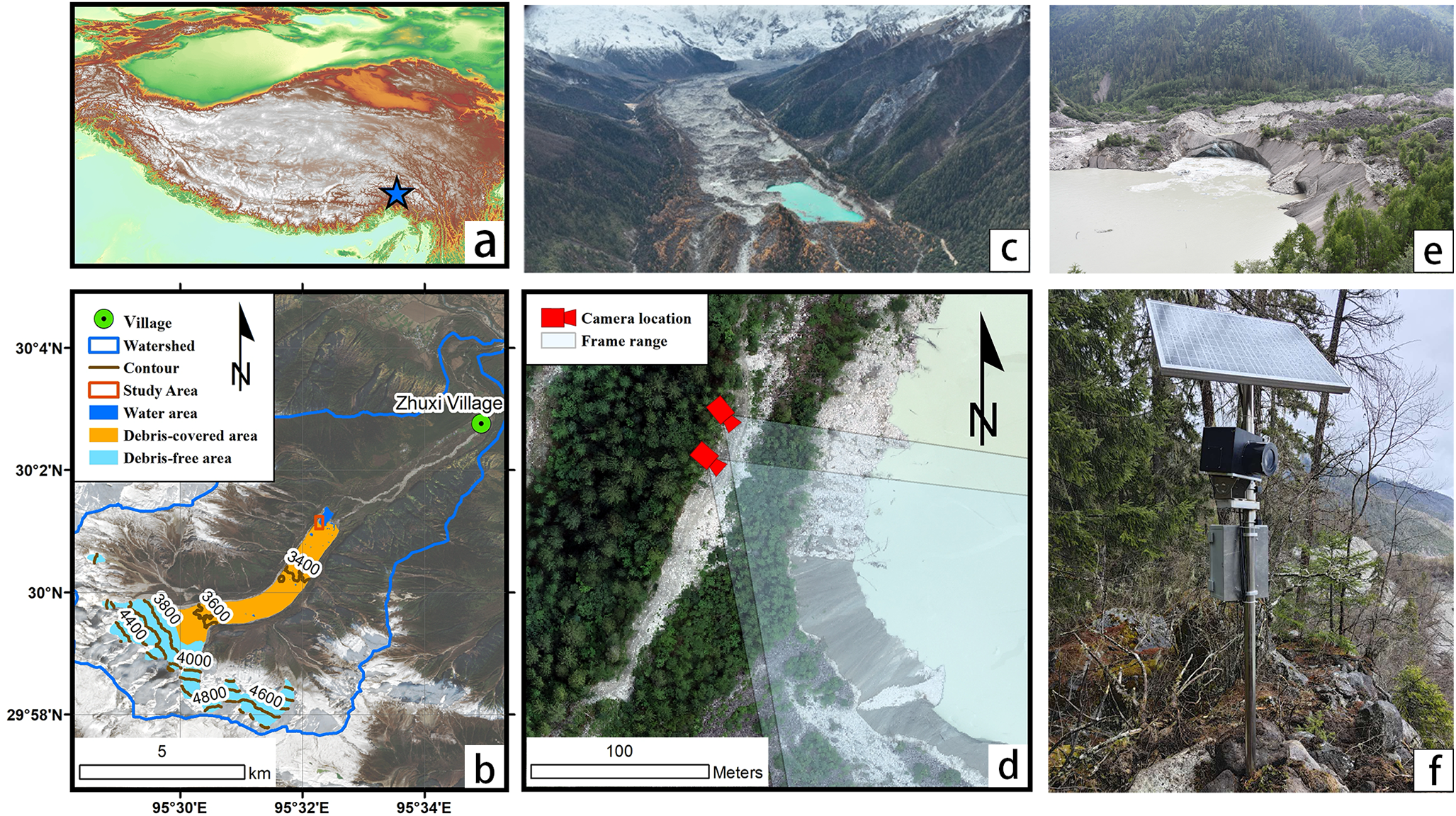
Figure 1. The location of Zhuxi glacier (a, b) and the specific study area. (c) Panoramic photo of Zhuxi glacier. (d) The location and frame range of two time-lapse cameras. (e) A sample photo. (f) The time-lapse camera setup. The background of (a) comes from Shuttle Radar Topography Mission (SRTM) while the background of (b) comes from Sentinel-2 image of July 2023.
The study ice cliff-pond system is geomorphologically complex in that it exhibits characteristics of both an ice cliff-pond assemblage but also bears similarities to larger, lake-terminating glacier termini. Our aim is to elucidate the dynamic interactions between supraglacial melt ponds and their attendant ice cliffs, as well as to examine the characteristics of the ice cliff-pond system as it transitions from a relatively small supraglacial melt hotspot to a much larger calving terminus bordering a proglacial lake. In doing so, we will generate data which could inform the advancement of numerical energy balance models, which can be used to reconstruct and predict ice cliff backwasting and meltwater contributions (Miles and others, Reference Miles, Pellicciotti, Willis, Steiner, Buri and Arnold2016; Buri and others, Reference Buri, Miles, Steiner, Immerzeel, Wagnon and Pellicciotti2016a; Buri and others, Reference Buri, Pellicciotti, Steiner, Miles and Immerzeel2016b). Our objectives are to: (1) apply SfM photogrammetry to create a time-series of detailed 3D points clouds of the ice cliff-pond system; (2) use 3D change detection to quantify rates and mechanisms of ice cliff backwasting, and track changes of the pond water level and (3) analyse the dynamic interactions between ice cliff evolution and melt pond hydrology.
2. Study area
Zhuxi Glacier extends from 5236 m a.s.l. to ∼3200 m a.s.l. and covers an area of ∼15 km2 (Fig. 1). Meltwater from the glacier supplies the Bodui Zangbo river, a tributary of the Yarlung Zangbo river. The glacier tongue below 3800 m a.s.l. is covered by a continuous debris layer with an average thickness of 0.54 ± 0.37 m (Rounce and others, Reference Rounce, Hock, McNabb, Millan, Sommer, Braun, Malz, Maussion, Mouginot, Seehaus and Shean2021). This debris layer becomes progressively thicker with decreasing altitude, exceeding 2 meters near the glacier’s terminus. While direct measurements of the thickest debris sections were impractical or unsafe, we visually assessed exposed debris profiles above ice cliffs in a UAV-derived point cloud to determine debris thickness ranging from 2 to 5 m.
Extensive debris cover, combined with a gentle slope averaging 4.3°, facilitates the development of numerous supraglacial ponds and ice cliffs on the glacier tongue. Based on the records of an Automatic Weather Station at 3250 m a.s.l. on the glacier terminus, the glacier, influenced by its low altitude and a monsoon-controlled climate, experiences high air temperatures (an annual mean of 7.1℃ in 2022) and substantial precipitation (1100 mm in 2022) compared to debris-covered glaciers elsewhere in the Himalayas.
According to UAV-based photogrammetry, the terminus ice cliff of Zhuxi Glacier is predominantly north-facing and exhibited an average slope of ∼40° and an area of ∼8100 m2 in August 2023. The cliff is adjacent to a melt pond which is the largest of all supraglacial ponds in the wider Zhuxi catchment with an area of 10.6 ± 0.8 × 10⁴ m2 in November 2023. The melt pond has expanded in area by a factor of ∼85 in the last decade and is closely monitored due to its potential for generating a future GLOF, which could pose a threat to downstream communities and infrastructure (He and others, Reference He, Yang, Wang, Zhao, Ren and Li2023).
3. Data and methods
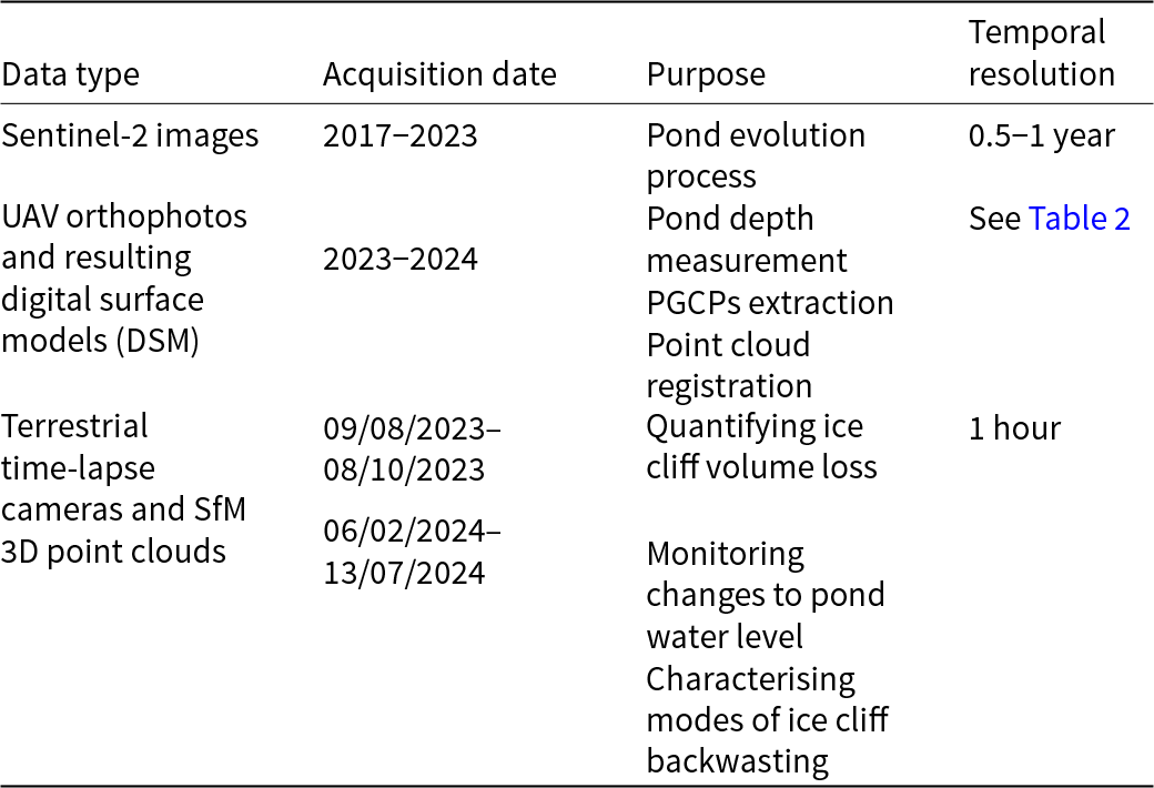
Three kinds of data were used or created in this study: (1) satellite imagery, (2) UAV imagery and (3) time-lapse photographs (Table 1). Satellite imagery was employed to monitor long-term changes in pond area. UAV-derived orthophotos and photogrammetrically derived digital surface models (UAV-DSM) served multiple purposes, including the measurement of (drained) pond depth and the extraction of ground control points with which to georeference 3D point clouds derived from time-lapse SfM photogrammetry. These time-lapse-derived 3D point clouds were in turn differenced to calculate ice cliff volume loss and pond water level change at high spatiotemporal resolution, enabling analysis of ice loss mechanisms.
Table 1. Datasets used in this study.
3.1. Satellite imagery
A total of 13 Sentinel-2A images were collected from 2017 to 2023 (Table 1). During this period, the normalised difference water index (NDWI) (Gao, Reference Gao1996) was calculated for each image to identify water bodies (Fig. 2). For this study, an NDWI threshold of 0.3 was applied to manually delineate pond boundaries in autumn (Taylor and others, Reference Taylor, Carr and Rounce2021), while a threshold of 0.2 was used in winter to account for the effects of snow and ice cover. We assume that the uncertainty in mapped pond area is accounted for by including a ±0.5 pixel boundary area (Salerno and others, Reference Salerno, Thakuri, D’Agata, Smiraglia, Manfredi, Viviano and Tartari2012).
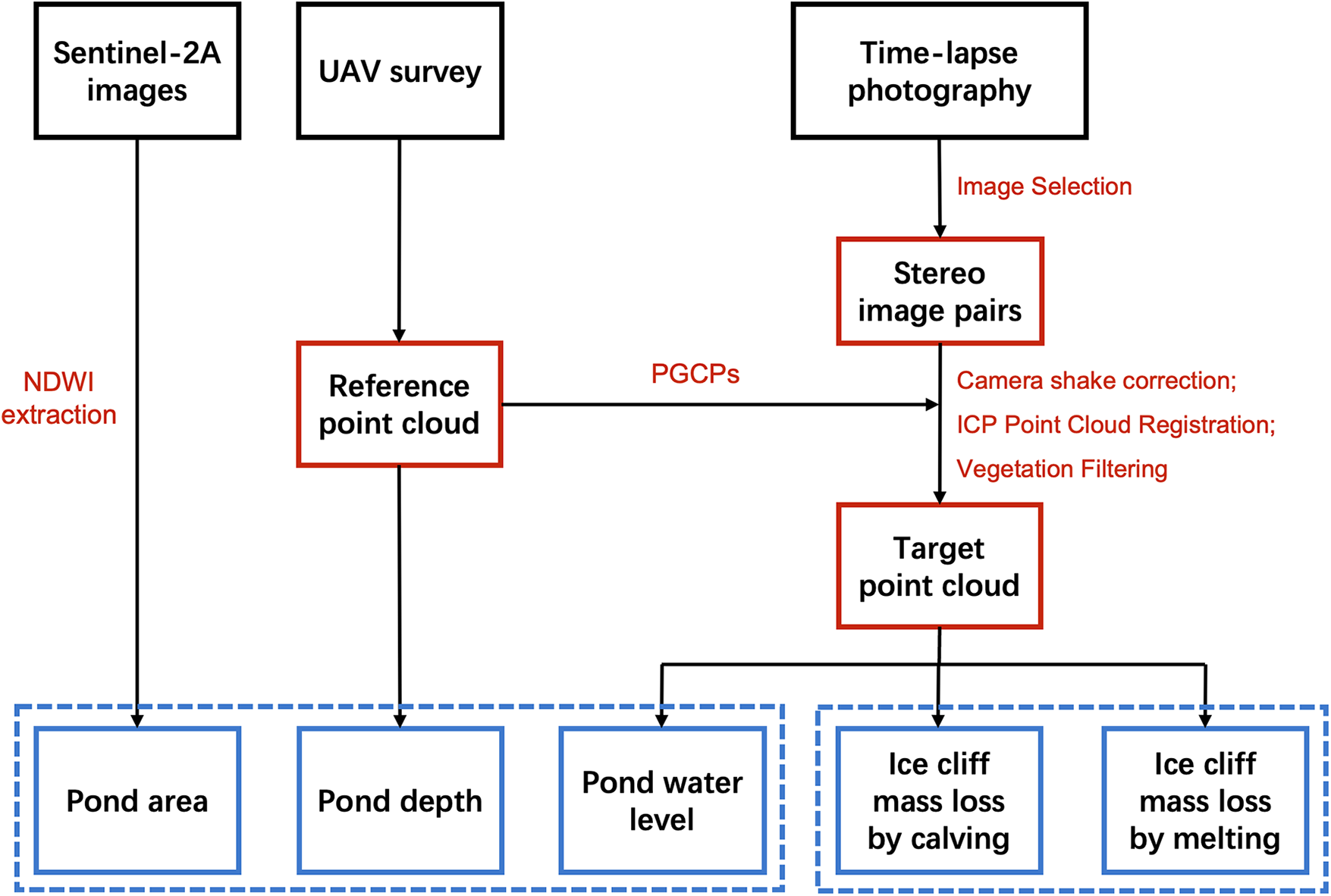
Figure 2. The workflow of ice cliff-pond system analysis. The black rectangles show the raw data, while the red rectangles show the intermediate data with relevant method. The results classified by blue dash line of pond and ice cliff are shown as blue rectangles.
3.2. UAV survey and post-processing
In April and August 2023, UAV surveys were carried out using a DJI Phantom 4 real-time kinematic (RTK) drone equipped with a 20 MP camera and RTK positioning. These flights were conducted at an above-ground elevation of 500 m and encompassed the debris-covered glacier area below 3600 m a.s.l. In July 2024, due to the failure of the DJI Phantom 4 RTK, the survey was conducted using a DJI Matrice 300 RTK platform with a Zenmuse L1 payload, which integrates a LiDAR module and a 20 MP RGB mapping camera on a 3-axis stabilised gimbal. For this study, only the RGB camera data was used, as the LiDAR module was unable to cover the entire study area. The DJI Matrice survey employed a terrain-following flight mode, maintaining a consistent distance of 120 m above ground level. The relevant information of UAV surveys is listed in Table 2.
Table 2. UAV surveys in this study.

The SfM software Pix4D Mapper (version 4.3.31) was employed for generating orthoimages and extracting point clouds from the three UAV surveys. The resolution of the SfM-derived orthophotos in two surveys were 0.14–0.42 m in 2023 and 0.10 m in 2024. The August 2023 UAV survey served as the reference dataset for spatial alignment. Co-registration of the three surveys was achieved by (1) horizontal (XY) alignment using six stable off-glacier control points identified in orthophotos and (2) vertical (Z) adjustment based on off-glacier bare terrain surfaces in DSMs (Yang and others, Reference Yang, Zhao, Westoby, Yao, Wang, Pellicciotti, Zhou, He and Miles2020; Karimi and others, Reference Karimi, Sheshangosht and Roozbahani2021; Zhao and others, Reference Zhao, Yang, Miles, Westoby, Kneib, Wang, He and Pellicciotti2023).
The UAV survey in April 2023 was carried out when the study melt pond was almost fully drained, exposing most of the pond bed. This allowed for the calculation of pond depth during the monsoon season based on the exposed pond bed altitude (Fig. 2) and the water level in monsoon season 2023 (3199.4 m a.s.l. on 9 August 2023) (Fig. 6a), the first water level we record since this UAV survey. The remaining pond area observed in April 2023 was treated as a ‘no data’ zone, since there is no pond bed elevation data recorded in this area.
The point clouds derived from UAV data in August 2023 and July 2024 were used as reference sets for aligning point clouds derived from SfM photogrammetry applied to the time-lapse camera imagery (Fig. 2). The August 2023 UAV survey coincided with the start of the first time-lapse camera study period, while the July 2024 survey corresponded to the end of the second time-lapse camera study period. To establish pseudo-ground control points (PGCPs), the UAV-derived point clouds were set to the same viewing angle as the time-lapse camera images in CloudCompare (version 2.13.2). A total of 40 PGCPs were selected in 2023 and 31 in 2024. The xyz coordinates, as well as the row and column positions of each PGCP in the time-lapse photos, were recorded and imported for subsequent data processing step.
3.3. Terrestrial photogrammetry and post-processing
Two time-lapse cameras were installed atop the lateral moraine crest on the west side of the pond (Fig. 1c,d). Each system consists of a Nikon D7500 camera (48 MP resolution, 18 mm lens), powered by a 5 W solar panel and a lithium-ion battery, with a solar charge controller. The camera is housed in a custom waterproof casing mounted beneath the solar panel, while other components are stored in a separate waterproof case strapped on a 2-meter-high aluminium mast (Fig. 1e). The cameras were configured to take simultaneous photographs hourly during daylight hours—this is a higher frequency than required, but provides ample data redundancy to mitigate, for example, short periods of low cloud obscuring the scene.
The overall workflow for processing time-lapse photography at Zhuxi Glacier is adapted from previous studies (Mallalieu and others, Reference Mallalieu, Carrivick, Quincey, Smith and James2017; Kneib and others, Reference Kneib, Miles, Buri, Fugger, McCarthy, Shaw, Chuanxi, Truffer, Westoby, Yang and Pellicciotti2022) (Fig. 2). In this study, several new methods were implemented to enhance the accuracy of the final point cloud outputs, especially since only two time-lapse photography systems were in operation.
The first step involved selecting the appropriate images from the raw dataset. Two distinct periods of time-lapse photography were analysed. A total of 41 photo pairs were manually selected from 09 August to 08 October in 2023 (61 days) according to photo pair quality, with images taken at 03:00–05:00 on daily interval. A total of 20 photo pairs were selected between 06 February and 13 July in 2024 (158 days). The limited number of available images during this period was due to snow cover and increased camera mast shaking. Photo pairs were selected at approximately half-monthly intervals, with increased frequency during periods of ice cliff failure to ensure data continuity. A total of two temporal gaps feature in the study period: (1) no images were captured between 10 August and 29 August due to a temporary malfunction; and (2) no point clouds were generated between November 2023 and January 2024 due to extensive snow cover.
Photo pairs were imported into an automated processing pipeline using an adaptation of the Python script developed by Kneib and others (Reference Kneib, Miles, Buri, Fugger, McCarthy, Shaw, Chuanxi, Truffer, Westoby, Yang and Pellicciotti2022) and accommodating software updates to Agisoft Metashape Professional (version 2.1.0). The script automatically generates a point cloud for each photo pair, utilising the xyz coordinates and row–column indices of PGCPs, as well as the location, azimuth, rotation and pitch angles of the time-lapse cameras.
Due to mast-shaking, the Python script required further adjustments. The shaking caused the row and column indices of PGCPs to shift across photo pairs, making it necessary to incorporate a camera shake correction process. This correction used a reference image with known PGCP positions to compute a transformation matrix based on feature matching between the reference and target images. The matrix was then applied to align the PGCP positions in subsequent images. It is worth noting that this correction could not be applied when most of the study area was snow-covered, necessitating manual adjustment of PGCP positions for three photo pairs captured in early February.
Additionally, the topographic noise in each time-lapse point cloud needed to be removed. For vegetation, Metashape’s in-built point cloud classification tool can divide point cloud into bare ground, ‘high’, ‘medium’ and ‘low’ vegetation. In this study, high and medium vegetation were excluded. Topographic noise in water-covered regions was manually removed using CloudCompare software (version 2.13.2). Following these steps, only the point clouds representing the ice cliff, adjacent debris-covered areas and other bare ground remained.
3.4. Ice cliff volume loss and water level of ponds
There are many ways to reconstruct ice cliff melt rates using point cloud data. One widely used approach is the Multiscale Model to Model Cloud Comparison (M3C2) method (Lague and others, Reference Lague, Brodu and Leroux2013), which calculates the 3D distance between two point clouds along the normal surface direction. This technique has been applied to analyse the melt distribution on glacier surfaces (Mishra and others, Reference Mishra, Miles, Chaudhuri, Mainali, Mal, Singh and Tiruwa2021) and ice cliffs (Watson and others, Reference Watson, Quincey, Carrivick and Smith2017). In this study, M3C2 was utilised to compare the retreat patterns of the ice cliff across different periods, providing data suitable for distinguishing ice loss due to melting versus structural collapse.
We divided the ice cliff into a ‘melting area’ and ‘calving area’ based on the position of crevasses. Within each area we used a different method for quantifying ice cliff volume loss: we used DEM differencing for calculating volume loss in the melting area, and 2.5D point cloud volume calculations for calculating volume loss in the calving area. DEM differencing is a method widely applied in glacier studies (Buri and others, Reference Buri, Miles, Steiner, Immerzeel, Wagnon and Pellicciotti2016a; Karimi and others, Reference Karimi, Sheshangosht and Roozbahani2021; Kneib and others, Reference Kneib, Miles, Buri, Fugger, McCarthy, Shaw, Chuanxi, Truffer, Westoby, Yang and Pellicciotti2022). DEMs for each time step were derived from point clouds using the rasterisation tool in CloudCompare. Because DEM differencing cannot capture ice volume loss in undercut sections of the cliff, we used 2.5D volume calculation tool in CloudCompare to estimate ice loss in these locations, including via structural collapse. This tool projects the ‘before’ and ‘after’ point clouds of the undercut surface onto a specific x-axis cross-section to obtain the distance between the point cloud and the reference plane. By measuring the distance difference and projected area between the two surfaces along the y-axis direction, the volume of the collapsed ice mass was calculated.
The resulting point clouds were also used to extract the elevation of the water surface, which was visually measured. For consistency, we recorded the elevation of the easternmost shoreline as the representative water level in this study.
3.5. Uncertainty
We employed final point cloud registration using CloudCompare’s Iterative Closest Point (ICP) algorithm (Open3D module) to improve the UAV co-registration and reduce the uncertainties associated with PCGP selection and glacier flow velocity. For ICP adjustment the UAV-derived point cloud was used as a reference and the debris-covered glacier surface immediately surrounding the study area was designated as the registration zone. We ignore the local sub-debris ice surface lowering rate of ∼0.05 cm d−1 (He and others, Reference He, Yang, Wang, Zhao, Ren and Li2023). This process also facilitated the correction of horizontal glacier flow (∼0.3 cm d−1) since the registration was conducted not only in the vertical direction but also in the horizontal direction on a sloped area. However, the use of only two cameras in this study resulted in lower accuracy in the final synthesised point clouds compared to other research (Mallalieu and others, Reference Mallalieu, Carrivick, Quincey, Smith and James2017; Kneib and others, Reference Kneib, Miles, Buri, Fugger, McCarthy, Shaw, Chuanxi, Truffer, Westoby, Yang and Pellicciotti2022). Consequently, varying degrees of geometric distortion occurred at different locations within the point clouds. Furthermore, due to the relatively minor ice cliff ablation in pre-monsoon season, 2024, we intentionally increased the temporal spacing between selected point clouds to ensure that the associated uncertainties remained within an acceptable range. Finally, a total of 17 point clouds in 2023 and 2024 were manually selected for volume loss calculations and subsequent process analysis.
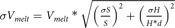
To estimate the uncertainties of volume loss in the melt-driven areas of the ice cliff, we consider the possible uncertainties from vertical thinning rates and ice cliff area measurements, both of which contributed to the overall uncertainty. The vertical thinning rates were derived from rasterised DSMs generated from the final registered point clouds. To assess the uncertainty in thinning rates, we selected a thick debris-covered glacier surface adjacent to the ice cliff as a check zone and calculated the standard deviation (STD) of elevation differences between each pair as σH (m). Throughout the study period, the melt area exhibited stable spatial extents (∼8100 m2 in August 2023 and ∼7700 m2 in July 2024). We applied a mean area of 7900 m2 as S and uncertainty range of ±200 m2 as σS for all volume loss calculations during the observation period. The resulting point cloud covered only 75% of the total known cliff area (∼6100 m2) and we make the assumption that our volume loss measurements are representative of, and can be extrapolate to, the wider cliff. Given the relatively high spatial homogeneity of ice cliff ablation observed in this study, the influence of uncertainties associated with this assumption can be neglected. The total uncertainty of volume loss rate σVmelt (m3/d) can be expressed as
 \begin{equation}\begin{array}{*{20}{c}}
{\sigma {V_{melt}} = {V_{melt}}*\sqrt {{{\left( {\frac{{\sigma S}}{S}} \right)}^2} + {{\left( {\frac{{\sigma H}}{{H*d}}} \right)}^2}}}
\end{array}\end{equation}
\begin{equation}\begin{array}{*{20}{c}}
{\sigma {V_{melt}} = {V_{melt}}*\sqrt {{{\left( {\frac{{\sigma S}}{S}} \right)}^2} + {{\left( {\frac{{\sigma H}}{{H*d}}} \right)}^2}}}
\end{array}\end{equation}where the Vmelt represents average volume loss in the melting area (m3/d), H represents average melt rate (m/d) and d represents the temporal interval in days.
The uncertainty quantification for both calving area volume loss and M3C2 distances utilises the same check zone as above. Given that this volume loss calculation is derived from the y-axis projection of the calving area, the final uncertainty of calving derived volume loss is determined by multiplying the STD of the y-axis distance in the check zone before and after failure by the projected area of the calving area onto the y-axis. The M3C2 distance uncertainty across the ice cliff equates to the STD of M3C2 measurements within the check zone between each image pair.
The uncertainty of melt pond water level mainly comes from two parts. The first is the accuracy of UAV-DSM. Though RTK and ICP registration improved the accuracy on relative position of UAV survey, this study did not use ground control points to ensure the absolute accuracy, which caused systematic error σsys range of 3 m in water level. The second part of uncertainty comes from the ICP registration (σICP) and UAV registration (σUAV), which were estimated from elevation differences STD from glacier surface check zone above and off-glacier check zone respectively. The total uncertainty of water level σW can be estimated as
 \begin{equation}\begin{array}{*{20}{c}}
{\sigma W = \,\sqrt {\sigma SY{S^2} + \sigma IC{P^2} + \sigma UA{V^2}}}
\end{array}\end{equation}
\begin{equation}\begin{array}{*{20}{c}}
{\sigma W = \,\sqrt {\sigma SY{S^2} + \sigma IC{P^2} + \sigma UA{V^2}}}
\end{array}\end{equation}4. Results
4.1. Pond development since 2017
Figure 3(a–d) shows the temporal evolution of the study proglacial pond over time. During 2017–2018, the pond had not yet fully formed, with only several small, isolated supraglacial ponds present in the area. These small ponds experienced a slight reduction in size during the post-monsoon season, contracting from a combined area of 1.14 ± 0.59 × 10⁴ m2 in November 2017 to 1.02 ± 0.54 × 10⁴ m2 in March 2018, before expanding to 1.96 ± 0.74 × 10⁴ m2 by October 2018. In the 2019 monsoon season, these smaller ponds coalesced, creating a single larger pond with an area of 5.34 ± 0.61 × 10⁴ m2, 2.7 times larger than the area of 2018.
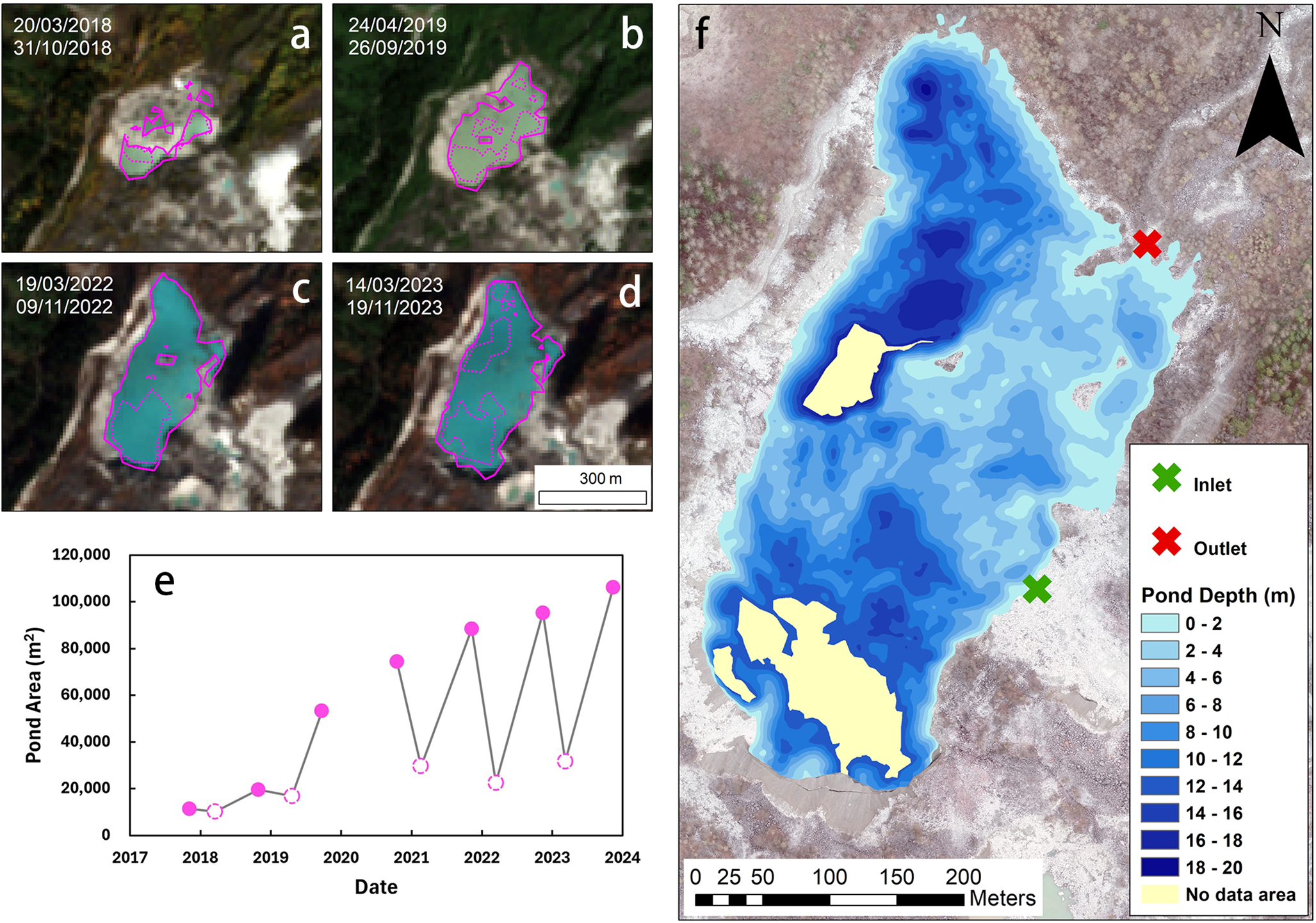
Figure 3. The evolution of proglacial pond during the period from 2017 to 2024, as well as the water depth in 2023. (a–d) The pond area before and after the monsoon season in 2018–19 and 2022–23. The pink solid line shows the area in Sep–Nov, and pink dash line shows the area in Mar–Apr. The background images come from Sentinel 2a images. (e) The seasonal change of pond area since 2017. (f) The pond depth derived from the UAV-DSM in Apr 2023. The ‘no data’ region corresponds to the pond’s extent in Apr 2024. A surface outlet is situated in the pond’s northeastern corner (red cross), while meltwater discharge flows into the pond from the east (green cross).
Since 2020, the pond has exhibited a pattern of substantial drainage during the non-monsoon period (December to March), followed by subsequent areal expansion in the monsoon season. In 2022, the pond’s area in March (2.26 ± 0.34 × 10⁴ m2) was only about a quarter of its area in November (9.53 ± 0.81 × 10⁴ m2). By March 2023, an increase in pond depth in the northwest (Fig. 3f) allowed for some water retention after its typical drainage, resulting in a larger pond area (3.17 ± 0.76 × 10⁴ m2) compared to previous years. After November 2023, the pond expanded further to 10.63 ± 0.79 × 10⁴ m2, with the main axis of expansion oriented northeast-southwest. However, since 2020, the north-eastward expansion of the pond has slowed considerably.
Figure 3f illustrates the water depth distribution of the pond during the 2023 monsoon season. The ‘no data’ region corresponds to the pond’s extent in April 2023, which is slightly smaller than its area in March (Fig. 3d). Mean depth of the pond is 7.29 m with maximum 19.09 m. The southern and northwestern sections of the pond reach depths exceeding 16 meters, while the northeastern portion remains shallower, at less than 10 meters. A surface outlet is situated in the pond’s northeastern corner in red cross, while meltwater discharge flows into the pond from the east (shown as a green cross in Fig. 3f).
4.2. Ice cliff changes in different seasons
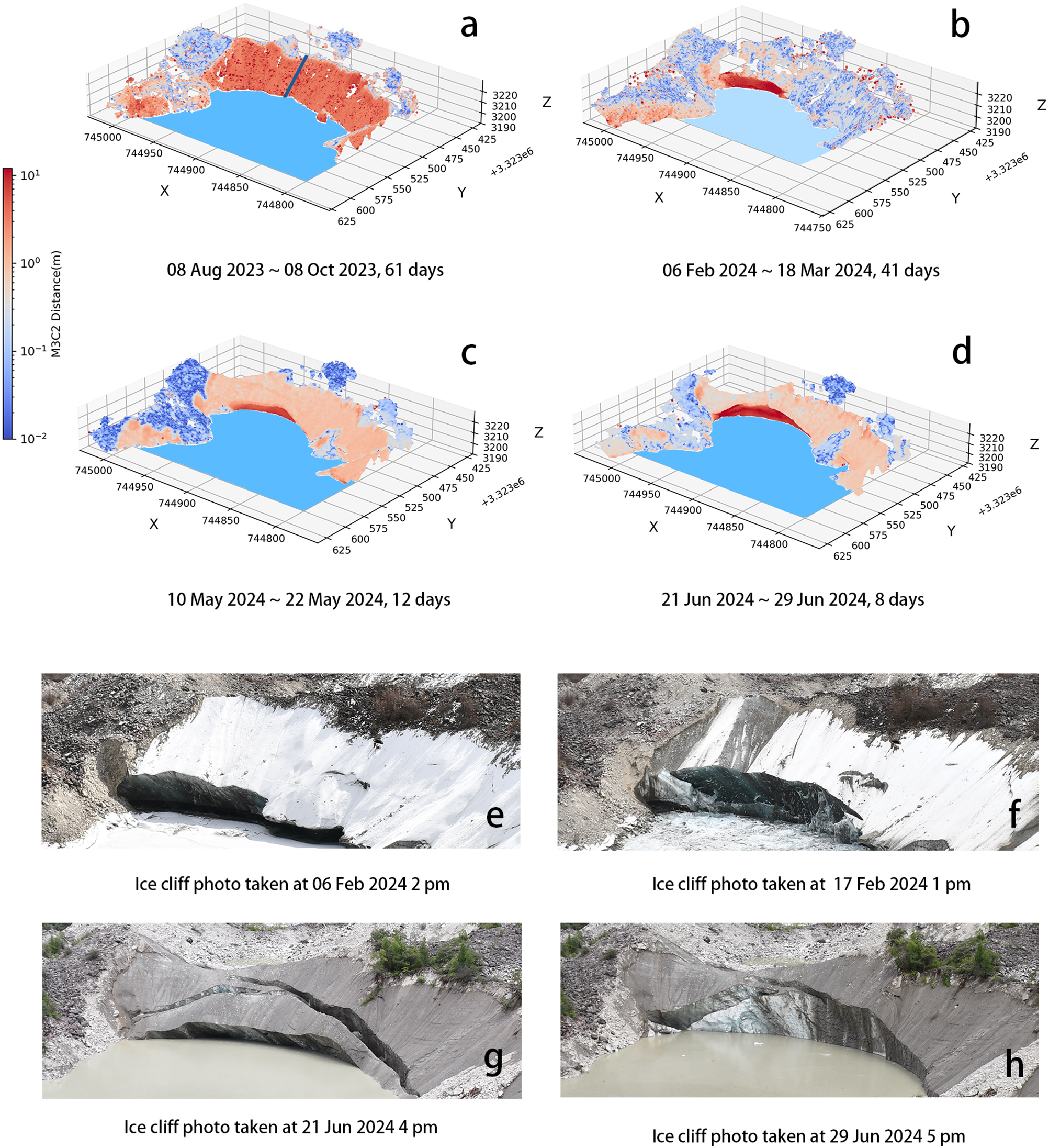
Figures 4 and 5 show the status of the ice cliff throughout the study period. During a 61-day period in August to October 2023 (Fig. 4a), the pond’s water level remained high at approximately 3200 m a.s.l., and the ice cliff backwasted in all directions by an average of 2.8 ± 0.2 m, or a daily mean rate of 4.6 ± 0.3 cm d−1.

Figure 4. M3C2 retreat distances of the study ice cliff across different periods in 2023 (a) and 2024 (b–d). The sections of Figure 5 are extracted in the location of the dark blue line in (a). The blue area in (a, c and d) shows the pond and the light blue area in (b) shows the frozen pond. (e–h) Photos of the ice cliff before and after mechanical failures in February and June.
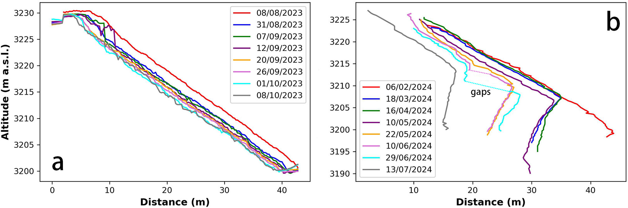
Figure 5. Change profiles of the ice cliff during the monsoon season of Aug–Oct 2023 (a) and pre-monsoon season of Feb–Jul 2024 (b). The section location is shown as dark blue line in Figure 4(a).
To highlight the importance of ice cliff failure, three intervals within the pre-monsoon season between February 6 and 21 June 2024 are selected in Fig. 4b–d. At least one mechanical ice cliff failure occurred in each interval. In the first interval from 6 February 2024 to 18 March 2024 (Fig. 4b), which lasted 41 days, the ice cliff was mostly snow-covered with less melting, resulting in a total of 0.2 ± 0.3 m backwasting with an equivalent melt rate of 0.6 ± 0.7 cm d−1. A collapse event during this period caused an instantaneous retreat of ∼15 m at the cliff base (Fig. 5b). During this interval, the proglacial pond was largely drained (the water level decreased from 3197.2 to 3189.2 m), leaving only shallow, frozen remnants near the cliff, visible as light blue in Fig. 4b.
In the second interval from 10 May 2024 to 22 May 2024 (Fig. 4c), the water level of the proglacial pond rose from 3913.2 ± 3.3 m to 3197.6 ± 3.3 m, and the ice cliff surface started to melt. An additional mechanical cliff failure occurred, resulting in an 8 m retreat of the cliff base. The lake was unfrozen during this period, and the ice cliff retreated by 0.6 ± 0.1 m over 12 days, or ∼ 5.1 ± 0.9 cm d−1—a retreat rate nine times that of the first interval.
In the third interval from 21 June 2024 to 29 June 2024 (Fig. 4d), the water level continued to rise, reaching approximately 3200.6 m a.s.l., with the retreat rate further accelerating to 7.1 ± 0.9 cm d−1, totalling 0.6 ± 0.1 m over 8 days. Two significant mechanical ice cliff failures occurred. Unlike the previous failures, these two events took longer; a rift first appeared on May 22, progressively enlarging over the next 31 days, leading to a 2 m advance at the cliff base (Fig. 5b). Following two major failures on June 22 and June 28, the ice cliff retreated an additional 10 m.
4.3. Ice loss with water level changes
Ice loss from the ice cliff during the 2024 pre-monsoon period occurred through progressive melting and ice cliff calving. Due to the rapid process of mechanical cliff failures, assessing ice loss purely based on retreat rates is insufficient. Simultaneously, the pond’s water level was monitored to evaluate its influence on ice cliff dynamics. Fig. 6 illustrates the melt rates of the ice cliff, water levels of the pond, and ice loss due to cliff calving during the study period, encompassing the late monsoon season of 2023 (Fig. 6a) and the pre-monsoon period of 2024 (Fig. 6b).
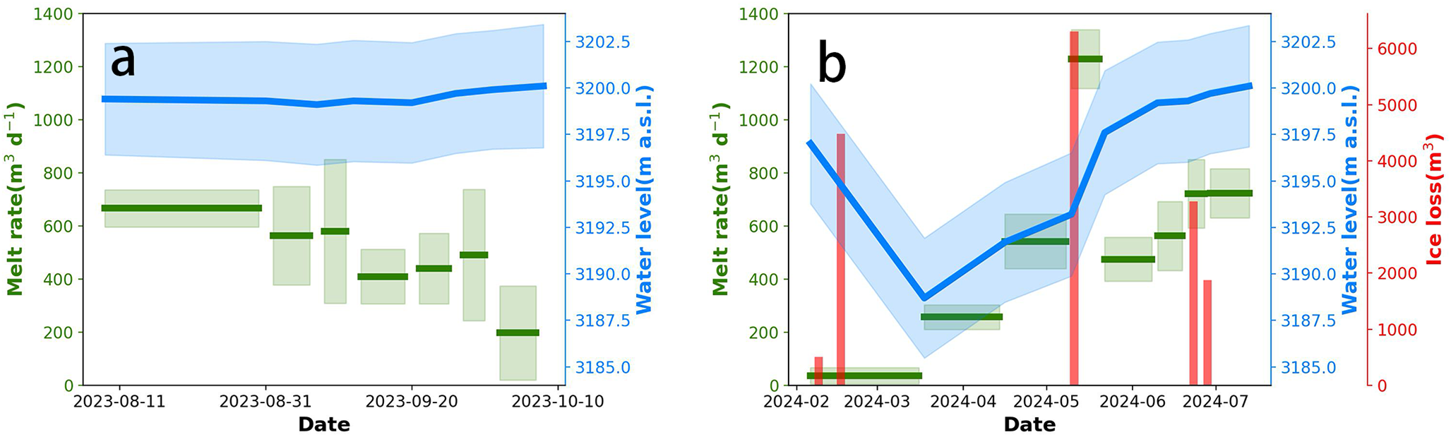
Figure 6. The melt rate of the ice cliff (m³ d−1), water level of the melt pond (m a.s.l.), as well as ice loss of the failure (m3) on the study ice cliff during 2023 (a) and 2024 (b). Uncertainty ranges for water level and melt rate measurements are indicated by light blue and light green shading, respectively.
In the late monsoon season of 2023, the melt rate of the ice cliff declined substantially, dropping 70.3% from 666.6 ± 66.6 m3 d−1 to 197.7 ± 164.1 m3 d−1 within 2 months. During this period, the pond’s water level remained relatively high (3200 ± 3 m a.s.l), and no cliff collapses were observed. In contrast, the ice cliff exhibited more complex dynamics during the 2024 pre-monsoon period; the melt rate showed a general increasing trend, from 36.9 ± 30.9 m3 d−1 to 724.1 ± 91.9 m3 d−1, with significant fluctuations in May—rising substantially to 1229.1 ± 112.8 m3 for 12 days before declining to 474.6 ± 81.6 m3 d−1. The total ice loss of ice cliff caused by melting in this period was 6.8 ± 1.2 × 10⁴ m3. The water level of the pond decreased by 8.3 ± 0.5 m between February and late March (3197 ± 3.2 m a.s.l. to 3188.7 ± 3.2 m a.s.l.) then increased by 11.4 ± 0.5 m (to 3200.1 ± 3.3 m) by mid-July. During this interval, five sizeable ice cliff failures were recorded, resulting in a total ice loss of 1.64 ± 0.07 × 10⁴ m3, and accounting for 19.5 ± 2.3 % of the total ice loss.
5. Discussion
5.1. Dynamic interactions between melt pond and ice cliff
During the pre-monsoon period, the dynamics of the pond, ice cliff melting and ice cliff calving exhibited complex interactions. In the monsoon season, ice cliff undercutting occurred below the waterline, leading to substantial ice loss (Watson and others, Reference Watson, Quincey, Carrivick and Smith2017). As a result of undercutting, the lower portions of the ice cliff were suspended above the water surface throughout the monsoon season (Watson and others, Reference Watson, Kargel, Shugar, Haritashya, Schiassi and Furfaro2020). As the pond’s water level dropped, this cantilevered section became unsupported, eventually leading to structural collapse.
Figure 6b highlights fluctuations in the pond’s water level and the melt rate of the ice cliff. Prior to late March, as the pond’s water level decreased to its lowest point the ice cliff’s melt rate also reached its minimum. Conversely, as the melt rate began to increase, the water level rose accordingly. Because ice cliffs can be a significant contributor to glacier mass loss (Sakai and others, Reference Sakai, Nakawo and Fujita1998; Brun and others, Reference Brun, Buri, Miles, Wagnon, Steiner, Berthier, Ragettli, Kraaijenbrink, Immerzeel and Pellicciotti2016; Buri and others, Reference Buri, Miles, Steiner, Ragettli and Pellicciotti2021), to some extent trends in the melt rate of a single ice cliff can serve as a useful indicator of temporal variations in meltwater production across the wider glacier system. This correlation between the ice cliff’s melt rate and the pond’s water level suggests that meltwater input is the primary driver behind the pond’s drainage dynamics. This correlation became particularly evident in mid-May: when the melt rate of the ice cliff surged to 1229.1 ± 111.3 m3 d−1, the pond’s water level increased by 4.4 ± 0.7 meters within just 12 days. After this period, the melt rate decreased to 400–800 m3 d−1, and the lake area was so large that a lower rate of meltwater input had little sustained effect on the pond’s water level.
5.2. Comparison with ‘classic’ supraglacial melt hotspots
Ice cliff-pond systems serve as key ablation hotspots for debris-covered glaciers, playing a crucial role in driving overall ice mass loss. Previous studies have demonstrated that ice cliffs exhibit ablation rates significantly higher than debris-covered areas (Reid and Brock, Reference Reid and Brock2014; Brun and others, Reference Brun, Buri, Miles, Wagnon, Steiner, Berthier, Ragettli, Kraaijenbrink, Immerzeel and Pellicciotti2016; Miles and others, Reference Miles, Steiner, Willis, Buri, Immerzeel, Chesnokova and Pellicciotti2017; Buri and others, Reference Buri, Miles, Steiner, Ragettli and Pellicciotti2021). At Zhuxi Glacier, the average elevation difference in ice cliff areas has been observed to be up to 6.6 times that of debris-covered areas (He and others, Reference He, Yang, Wang, Zhao, Ren and Li2023). The relationship between melt rates at these hotspots and at the supraglacial debris-ice interface determines the ablation enhancement factor of debris-covered glaciers compared to debris-free glaciers, and is important for large-scale glacier melt estimation (Miles and others, Reference Miles, Steiner, Buri, Immerzeel and Pellicciotti2022).
Ice cliff melt rates have been measured by many studies, using ablation stakes (Han and others, Reference Han, Wang, Wei and Liu2010; Reid and others, Reference Reid and Brock2014) or terrestrial photogrammetry (Watson and others, Reference Watson, Quincey, Carrivick and Smith2017; Kneib and others, Reference Kneib, Miles, Buri, Fugger, McCarthy, Shaw, Chuanxi, Truffer, Westoby, Yang and Pellicciotti2022). In this study, the ice cliff melt rate ranges from 0.5 to 9.2 cm d−1 from February to July—this is larger than the ice cliff melt rate on Khumbu Glacier (0.30–5.18 cm d−1; Watson and others, Reference Watson, Quincey, Carrivick and Smith2017) and Langtang Glacier (0.7–3.4 cm d−1; Kneib and others, Reference Kneib, Miles, Buri, Fugger, McCarthy, Shaw, Chuanxi, Truffer, Westoby, Yang and Pellicciotti2022) on the southern slope of the Himalayas, but similar to that of Koxkar Glacier in the Tien Shan (8 cm d−1 highest in July; Han and others, Reference Han, Wang, Wei and Liu2010), Miage Glacier in the European Alps (6.4–7.1 cm d−1 in June; Reid and others, Reference Reid and Brock2014), and 24K Glacier in southeast Tibet (1.1–6.7 cm d−1; Kneib and others, Reference Kneib, Miles, Buri, Fugger, McCarthy, Shaw, Chuanxi, Truffer, Westoby, Yang and Pellicciotti2022). The melt rate of ice cliffs across different glaciers was mainly controlled by their meteorological conditions. Zhuxi Glacier’s air temperature (daily average 15–20 ℃ in summer) is substantially higher than Khumbu and Langtang Glaciers (daily average 0–6 ℃ in summer; Watson and others, Reference Watson, Quincey, Carrivick and Smith2017; Kneib and others, Reference Kneib, Miles, Buri, Fugger, McCarthy, Shaw, Chuanxi, Truffer, Westoby, Yang and Pellicciotti2022), therefore driving a higher ice cliff melt rate.
Proglacial ponds also play a crucial role in maintaining ice cliff stability by facilitating continuous subaqueous calving, providing significantly higher backwasting rates compared to subaerial melting (Sakai and others, Reference Sakai2012; Miles and others, Reference Miles, Pellicciotti, Willis, Steiner, Buri and Arnold2016a). In this study, sustained expansion of an adjacent melt pond has driven persistent backwasting of the study ice cliff over 7 years (He and others, Reference He, Yang, Wang, Zhao, Ren and Li2023). Seasonal drainage of the melt pond revealed pronounced subaqueous undercutting and erosional notching, consistent with prior findings (Sakai and others, Reference Sakai, Takeuchi, Fujita and Nakawo2000; Röhl and others, Reference Röhl2006) (Fig. 4e–h).
The proglacial pond at Zhuxi Glacier has exhibited an annual pattern of draining and refilling since 2020. Previous studies have documented similar seasonal fluctuations in supraglacial ponds, noting that their number and area typically decline during the monsoon season and recover in the spring over HMA (Benn and others, Reference Benn, Bolch, Hands, Gulley, Luckman, Nicholson, Quincey, Thompson, Toumi and Wiseman2012; Salerno and others, Reference Salerno, Thakuri, D’Agata, Smiraglia, Manfredi, Viviano and Tartari2012; Watson and others, Reference Watson, Quincey, Carrivick and Smith2016; Miles and others, Reference Miles, Willis, Arnold, Steiner and Pellicciotti2016b; Narama and others, Reference Narama, Daiyrov, Tadono, Yamamoto, Kaab, Morita and Ukita2017). However, the proglacial pond in this study drained during the non-monsoon season in February rather than in the monsoon season, suggesting that its drainage and refilling are governed by a distinct control factor.
The drainage of ‘classic’ supraglacial ponds is primarily influenced by their connectivity to englacial conduits (Benn and others, Reference Benn, Wiseman and Hands2001; Benn and others, Reference Benn, Thompson, Gulley, Mertes, Luckman and Nicholson2017; Miles and others, Reference Miles, Steiner, Willis, Buri, Immerzeel, Chesnokova and Pellicciotti2017). In summer, meltwater re-establishes these conduits, facilitating pond drainage when the conduits connect (Liu and others, Reference Liu, Mayer and Liu2015; Narama and others, Reference Narama, Daiyrov, Tadono, Yamamoto, Kaab, Morita and Ukita2017). In some cases, conduits become blocked due to roof collapses caused by continuous melting, leading to pond refilling in subsequent years as meltwater accumulates (Sakai and others, Reference Sakai, Takeuchi, Fujita and Nakawo2000; Röhl and others, Reference Röhl2006, Reference Röhl2008; Miles and others, Reference Miles, Pellicciotti, Willis, Steiner, Buri and Arnold2016; Narama and others, Reference Narama, Daiyrov, Tadono, Yamamoto, Kaab, Morita and Ukita2017).
The drainage of the ice cliff-pond system at Zhuxi Glacier is driven by a number of mechanisms. When the lake almost fully drained in April 2023, some of the buried ice appeared at the lake bed, proving that the lake did not extend through the entire glacier ice thickness. The buried ice, as well as the drainage event in Fig. 6b, proves the existence of an englacial conduit. However, conduit connectivity does not appear to govern the drainage event in winter, as meltwater in winter is insufficient to re-establish it during that period. Furthermore, the stable high-water level during the 2023 monsoon season (Fig. 6a) suggests that this conduit was not re-established at that time either. In this case, we hypothesise the presence of a stable englacial conduit beneath the proglacial pond, which functions as an outlet that operates independently of the subaerial channel (shown in Fig. 3f). Compared with disconnected, stable supraglacial ponds, this proglacial pond appears to become stable in the monsoon season by achieving a water balance through continuous and unimpeded meltwater input and output; as discussed in Section 4.3, the water level of the pond is strongly correlated with meltwater input. The pond drains during the winter when meltwater input decreases and refills in the spring as meltwater input increases.
5.3. Comparison with proglacial calving termini and its future evolution
Though our ice cliff-pond system shares some similarities with supraglacial hotspots such as seasonally draining melt ponds and attendant ice cliffs, the location and calving process of our system also shows similarity with more ‘typical’ proglacial calving fronts, including frequent mechanical ice cliff failure and substantial thermo-erosional undercutting (Watson and others, Reference Watson, Kargel, Shugar, Haritashya, Schiassi and Furfaro2020).
With continual areal expansion and deepening, a series of multi-basin base-level supraglacial ponds can merge into a large moraine dammed lake (Thompson and others, Reference Thompson, Benn, Dennis and Luckman2012; Mertes and others, Reference Mertes, Thompson, Booth, Gulley and Benn2017). The base level of individual ponds can vary, even when ponds are in close proximity. The base level of proglacial lakes typically represents the lowest point within the entire glacial lake system, reducing the likelihood of sudden drainage events (Watanabe and others, Reference Watanabe, Lamsal and Ives2009; Miles and others, Reference Miles, Hubbard, Quincey, Miles, Irvine-Fynn and Rowan2019, Reference Miles, Hubbard, Irvine-Fynn, Miles, Quincey and Rowan2020). A proglacial lake receives the majority of its meltwater input from upstream, which promotes lake expansion and drives the calving of adjacent ice cliffs (Thakuri and others, Reference Thakuri, Salerno, Bolch, Guyennon and Tartari2016; Benn and others, Reference Benn, Thompson, Gulley, Mertes, Luckman and Nicholson2017). Meanwhile, persistent subaqueous undercutting can, in some cases, cause these lakes to erode through the entire glacier thickness, reaching down to the bedrock and enabling further expansion (Watanabe and others, Reference Watanabe, Lamsal and Ives2009).
This study’s ice cliff-pond system exhibits both similarities to and differences from a proglacial calving front. At the early stage of system development (Fig. 3a), a larger pond forms through the coalescence of several smaller ponds, eventually evolving into a larger proglacial pond. Since 2020, this system has been receiving nearly all upstream meltwater (He and others, Reference He, Yang, Wang, Zhao, Ren and Li2023), mirroring the characteristics of a proglacial lake. However, an englacial conduit persists beneath the pond, causing annual drainage and subsequent refilling. The unstable water level of this pond results in a distinct backwasting mechanism for the adjacent ice cliff, differing between the monsoon and non-monsoon seasons.
Although the calving mechanism of the Zhuxi Glacier’s ice cliff during the non-monsoon season is similar to that observed in previous studies—being driven by continuous undercutting and suspended ice (Kirkbride and Warren, Reference Kirkbride and Warren1997; Sakai and others, Reference Sakai2012) — the volume of calved ice from Zhuxi Glacier is substantially smaller. For instance, Watson and others investigated calving events at debris-covered Thulagi Glacier, which is of a similar size to Zhuxi Glacier. Their findings indicated a calved volume of approximately 4.87 × 10⁵ m3 between April and September, significantly exceeding our study’s result of 1.48 × 10⁴ m3 (February to July). Thulagi Lake is approximately ten times larger in surface area (9.3 × 10⁵ m2) and four times deeper (76 m) than the pond associated with Zhuxi Glacier, resulting in a larger contact area between the lake and adjacent ice cliff, and likely a more complex pattern of water circulation. Similarly large, ‘mature’ calving fronts are widespread across HMA (Westoby and others, Reference Westoby, Glasser, Brasington, Hambrey, Quincey and Reynolds2014; Taylor and others, Reference Taylor, Robinson, Dunning, Rachel Carr and Westoby2023), contributing to significant ice loss in the region (Zhang and others, Reference Zhang, Bolch, Yao, Rounce, Chen, Veh, King, Allen, Wang and Wang2023). Given that it currently retains some characteristics of supraglacial hotspots, such as seasonal drainage ponds and melt-controlled ice cliffs during the monsoon season, Zhuxi Glacier appears to be in the early stages of proglacial calving front development.
The future evolution of Zhuxi Glacier’s ice cliff-pond system could present a significant concern, particularly its potential for generating a glacial lake outburst flood (GLOF), a hazard commonly associated with proglacial moraine dammed lakes. At present, ice cliff failures at the terminus of the Zhuxi Glacier predominantly occur during the pre-monsoon season when the pond’s water level is relatively low. This seasonal pattern mitigates one of the primary GLOF triggers, namely sudden wave overtopping of a moraine dam (Westoby and others, Reference Westoby, Glasser, Brasington, Hambrey, Quincey and Reynolds2014). Additionally, the pond’s area remains considerably smaller compared to more mature proglacial moraine-dammed lakes, further reducing the current GLOF hazard. However, ongoing ice cliff backwasting and pond undercutting may lead to the coalescence of the proglacial pond with other supraglacial ponds (Thompson and others, Reference Thompson, Benn, Dennis and Luckman2012; He and others, Reference He, Yang, Wang, Zhao, Ren and Li2023). Such a process could result in the erosion of the glacier’s entire thickness, disrupt the seasonal drainage cycle and increase the future GLOF risk for downstream regions. We recommend continued monitoring of the study area in the context of future GLOF hazard.
5.4. Conceptual model of the ice cliff-pond system
Defining this ice cliff-pond system on Zhuxi Glacier as either a classic supraglacial hotspot or a proglacial calving front proves challenging because it currently exhibits characteristics of both systems, as we mentioned in Sections 5.2 and 5.3. We define this ice cliff-pond system as being in a transitional stage between a supraglacial hotspot and a proglacial calving front. This evolution from a supraglacial pond into a proglacial lake has been widely described in previous studies (Benn and others, Reference Benn, Bolch, Hands, Gulley, Luckman, Nicholson, Quincey, Thompson, Toumi and Wiseman2012; Mertes and others, Reference Mertes, Thompson, Booth, Gulley and Benn2017; Miles and others, Reference Miles, Hubbard, Irvine-Fynn, Miles, Quincey and Rowan2020). However, we also observe some features characteristic of this transitional stage which are not mentioned in previous studies, including the meltwater-controlled drainage-refill cycle and contrasting primary ice cliff backwasting mechanisms during monsoon and non-monsoon seasons. Informed by our findings, we present a conceptual model to illustrate the annual cycle of this distinctive ice cliff-pond system (Fig. 7).
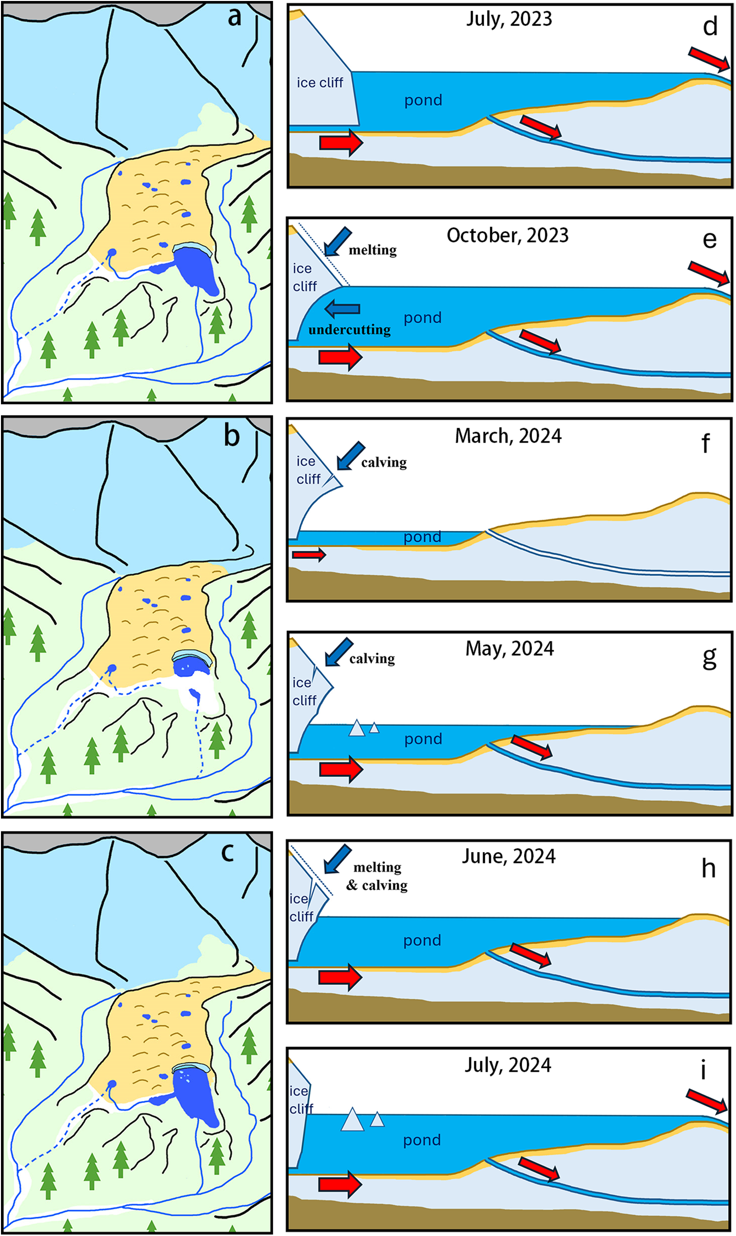
Figure 7. Conceptual model of the ice cliff-pond system, including the monsoon season in Jul–Oct 2023 (a), non-monsoon season in Mar–May 2024 (b), and monsoon season in July 2024 (c). The section of ice cliff-pond system of the study period shows in (d–i). The blue arrows show the melting and calving process of ice cliff, the different sizes of red arrows show the amount of meltwater flux.
Figure 7a presents the diagram of the terminus of Zhuxi Glacier during the monsoon season (July to October 2023), highlighting the ice cliff-pond interaction. The blue dash line marks the former proglacial meltwater channel that dried up in the summer of 2020 when a new channel diverted meltwater into the study pond. The proglacial stream outlet in Fig.3f is also shown in Fig.7a. This outlet, situated at an elevation of 3198 m a.s.l., indicates that when the pond’s water level drops below this threshold, the surface stream dries up, leaving the pond without a visible surface outlet. The study pond recorded a minimum water level of 3188.7 m a.s.l., suggesting the presence of an englacial conduit as a secondary outlet in addition to the proglacial stream. Meanwhile, another englacial conduit may also exist underneath the ice cliff, which can play an important role for supplying meltwater.
In the monsoon season (July to October), the study pond maintains a balance between meltwater inflows and outflows via two inlets and two outlets. The pond’s water level remains consistently high, while the adjacent ice cliff undergoes melting and calving (Fig. 6e), resulting in substantial ice loss. In late winter (February to March), as illustrated in Fig. 7b and f, a decrease in meltwater input leads to drainage, causing the pond’s water level to drop to the elevation of its englacial conduit outlet. During this period, both the proglacial stream channel and pond surface stream dry up due to reduced meltwater inflow. With colder temperatures, melting slows significantly, and ice loss is primarily driven by ice cliff failures, which occasionally produce small icebergs on the pond’s surface.
As the air temperature begins to rise after March (Fig. 7g,h), meltwater input increases and the water level starts to rise. In this period, the pond receives meltwater from both the surface stream and inlet englacial conduit, resulting in a net gain since meltwater outflow through the englacial conduit alone cannot match the increased inflow. In this period, ice cliff mass loss is driven by a combination of melting and calving events. By July 2024, with the onset of monsoon season, the pond’s water level returns to its peak (Fig.7c,i), restoring the ice cliff-pond system to conditions similar to those in July 2023. This annual drainage-refill cycle causes the pond to expand southward as continued ice cliff melting and failures reshaping the landscape.
Comparative analysis with other glaciers can elucidate the underlying causes of this unique process above. Specifically, the processes governing ice cliff melt and calving process have been thoroughly investigated in previous Himalayan studies (Buri and others, Reference Buri, Miles, Steiner, Immerzeel, Wagnon and Pellicciotti2016a; Watson and others, Reference Watson, Kargel, Shugar, Haritashya, Schiassi and Furfaro2020; Buri and others, Reference Buri, Miles, Steiner, Ragettli and Pellicciotti2021). However, to the best of our knowledge the seasonal alternation between melting and calving in this particular system—which arises as a direct consequence of periodic water level fluctuations in the adjacent melt pond—has not been observed elsewhere. These seasonal water-level variations are primarily driven by the presence of stable subglacial meltwater channels, which in turn reflect the stagnant characteristics of the glacier’s terminus. This stagnation prevents ice flux during the ablation season from influencing channel connectivity, unlike in more dynamically active glaciers (Liu and others, Reference Liu, Mayer and Liu2015; Narama and others, Reference Narama, Daiyrov, Tadono, Yamamoto, Kaab, Morita and Ukita2017). Notably, many glaciers with a stagnant terminus have developed large proglacial lakes with bedrock bases, where subglacial meltwater channels are absent, and thus no significant seasonal water-level fluctuations occur (Thompson and others, Reference Thompson, Benn, Dennis and Luckman2012; Mertes and others, Reference Mertes, Thompson, Booth, Gulley and Benn2017; Miles and others, Reference Miles, Hubbard, Irvine-Fynn, Miles, Quincey and Rowan2020). The transitional state in this study is not a long-term sustainable condition. As the underlying ice beneath the lake gradually erodes, the system is expected to evolve into a conventional proglacial moraine-dammed lake. Similar transitional states may have occurred in other debris-covered glaciers with stagnant termini, but these transitions likely did not persist for more than 5 years—unlike Zhuxi Glacier—and thus have not been observed. This prolonged transitional state in the Zhuxi Glacier may be attributed to a lower melt rate or greater ice thickness beneath the lake. However, there is currently no direct evidence to support this hypothesis. Continued monitoring of the system’s future development is necessary to validate our interpretation.
5.5. Future research directions
The unique seasonal dynamics of the ice cliff-pond system offer valuable insights for future advancements in related modelling efforts. Existing models of the energy balance of supraglacial ponds have often overlooked events such as drainage or changes in pond area and volume, leading to inaccuracies when modelling over longer periods (Miles and others, Reference Miles, Pellicciotti, Willis, Steiner, Buri and Arnold2016). To improve model accuracy, incorporating estimates of pond area variation is crucial. This study identifies a previously unreported drainage-refill cycle, providing a new avenue for refining energy balance models, and beyond the summer drainage events commonly depicted in earlier studies.
While this study has elucidated the mechanisms underlying the seasonal dynamics of the ice cliff-pond system, the contribution of subaqueous undercutting to ice loss remains unquantified, despite its recognised significance (Watson and others, Reference Watson, Kargel, Shugar, Haritashya, Schiassi and Furfaro2020). Fortunately, the seasonal drainage of the pond presents an opportunity to quantify subaqueous undercutting by comparing the ice cliff’s state before and after refill events, as more data become available in the future. Data obtained from alternative surveying methods such as terrestrial laser scanning (Singh and others, Reference Singh, Vijay, Banerjee, Sarangi, Rashid and Zargar2025) and ground penetrating radar (Mertes and others, Reference Mertes, Thompson, Booth, Gulley and Benn2017) may also help us to quantify ice loss associated with these features.
Future studies should also compare these observations with existing ice cliff energy balance models, which may partly explain the melt rate dynamic in the pre-monsoon season. However, current models do not fully account for the influence of adjacent ponds, including their microclimatic effects on melting and their role in subaqueous undercutting and calving (Buri and others, Reference Buri, Miles, Steiner, Immerzeel, Wagnon and Pellicciotti2016a; Buri and others, Reference Buri, Pellicciotti, Steiner, Miles and Immerzeel2016b). This study highlights an underestimated ∼19.5% ice loss due to calving, distinct from melting during the pre-monsoon season, which is not captured by existing models. While the monsoon-season backwasting process of the study’s ice cliff aligns more closely with previous model predictions, the adjacent pond likely exerts a microclimatic influence on the melting rate, necessitating further investigation.
6. Conclusion
As glaciers retreat, the interaction between supraglacial ponds and ice cliffs plays a pivotal role in driving ice loss, especially through seasonal calving and melting processes. Understanding the seasonal fluxes that govern ice cliff retreat—such as the seasonal drainage and refilling of ponds—can ultimately improve our predictions of glacier behaviour. We used satellite imagery and time-lapse terrestrial photogrammetry to quantify the dynamics of an ice cliff-pond system on Zhuxi Glacier, southeastern Tibet. This system, which is transitioning from a supraglacial melt hotspot to a proglacial calving front, displays complex seasonal interactions between the pond and its adjacent ice cliff. Our findings reveal a link between the pond’s water level and the ice cliff’s melt rate, with meltwater supply driving both pond drainage and refilling. Notably in the pre-monsoon season (February to July 2024), ice cliff failures accounted for ∼19.5% of total ice loss—an often-overlooked factor in numerical ice cliff models. This study contributes to a deeper understanding of the mechanisms which drive ice cliff evolution and glacial lake development, emphasising the need for more comprehensive models that incorporate both surface processes and subaqueous interactions.
Data availability statement
The Python scripts to processing of the time-lapse photos to point clouds, as well as ICP registration, are available on Zenodo (https://doi.org/10.5281/zenodo.16272541).
Acknowledgements
This study was supported by the National Natural Science Foundation of China (Grant Nos. 42271138, 42201144), Lhasa Science and Technology Plan Project (LSKJ202406), the National Key R&D Program of China (Grant No. 2024YFF0808601) and the Science and Technology Plan Projects of Tibet Autonomous Region (Grant Nos. XZ202501ZY0081 and XZ202401ZY0003). ZH additionally acknowledges mobility funding provided by China Scholarship Council (CSC), supporting an extended research stay at the University of Plymouth, where much of this research was completed.
Competing interests
The authors declare that they have no competing interests.


 Open access