


Over the last couple of decades, both political scientists and policymakers have become increasingly concerned about affective political polarization. This describes the phenomenon of people from different political groups, primarily partisans, not just disagreeing, but also becoming hostile to one another. Increasing affective partisan polarization in the United States (US) has been well documented (Iyengar et al., Reference Iyengar, Lelkes, Levendusky, Malhotra and Westwood2019; Iyengar & Westwood, Reference Iyengar and Westwood2015; Mason, Reference Mason2015, Reference Mason2018), but comparative work suggests that these dynamics of in-party affinity and out-party animosity are just as pronounced in many other democracies (Gidron et al., Reference Gidron, Adams and Horne2020; Harteveld, Reference Harteveld2021a; Reiljan, Reference Reiljan2020; Wagner, Reference Wagner2021). Other political divides than partisanship can also give rise to similar tensions (Zollinger, Reference Zollinger2024). Among the most prominent of these has been the intense polarization between Leavers and Remainers over Brexit in the United Kingdom (UK) since the 2016 referendum (Curtice, Reference Curtice2018; Hobolt et al., Reference Hobolt, Leeper and Tilley2021; Kenny et al., Reference Kenny, Heath and Richards2023). Given democratic politics requires compromise by both sides and a willingness to accept defeat by the losing side, entrenched hostilities between political groups are worrying since they may prevent both the acceptance of compromise and defeat (Iyengar et al., Reference Iyengar, Lelkes, Levendusky, Malhotra and Westwood2019; Kingzette et al., Reference Kingzette, Druckman, Klar, Krupnikov, Levendusky and Ryan2021).
Understanding why there is affective polarization is thus critical. There is good evidence that ideological and social sorting increase affective polarization (Mason, Reference Mason2018). That is, when people on different sides of a political divide are different to one another, both in terms of their ideology and other important social identities such as religion, class and race, there is greater affective polarization. There are, therefore, at least two legs to the stool that supports the emergence of affective polarization. When parties present more ideologically coherent platforms, this leads to ideological sorting (Levendusky, Reference Levendusky2009) and when social identities are more aligned with one another, this leads to social sorting (Harteveld, Reference Harteveld2021b; Mason, Reference Mason2018). Yet there is an oft-mentioned, but never tested, third leg to the stool: geographical sorting.
On this account, the political homogeneity of neighbourhoods plays an important role in affective polarization by creating more, or fewer, interactions with people on the other side of the political divide. For example, discussing the increasing levels of affective polarization in the US, Lelkes and Westwood (Reference Lelkes and Westwood2017, p. 490) suggest that the ‘increase in social distance may be related to the actual geographical distance that has grown between partisans’. These concerns about the link between geographical sorting and polarization are not new: Butler and Stokes were writing about these effects in Britain in the 1960s (Butler & Stokes, Reference Butler and Stokes1974; see also Fitton, Reference Fitton1973; Johnston & Pattie, Reference Johnston and Pattie2006). Nonetheless, they came to greater prominence after Bill Bishop's book The Big Sort, in which he argued that Americans had become more likely to live in politically homogenous neighbourhoods (Bishop, Reference Bishop2009; Brown & Enos, Reference Brown and Enos2021; Johnston et al., Reference Johnston, Manley and Jones2016; Rohla et al., Reference Rohla, Johnston, Jones and Manley2018; although see Abrams & Fiorina, Reference Abrams and Fiorina2012). Either people are selecting into neighbourhoods because of their politics (Gimpel & Hui, Reference Gimpel and Hui2015; Tam Cho et al., Reference Tam Cho, Gimpel and Hui2013) or the type of factors that predict where people choose to live, such as wealth, also predict partisanship (Johnston et al., Reference Johnston, Manley and Jones2016; Martin & Webster, Reference Martin and Webster2020; Mummolo & Nall, Reference Mummolo and Nall2017). Both mechanisms bolster attachments to the party that is dominant in an area and this geographical sorting leads to even greater local political homogeneity (Martin & Webster, Reference Martin and Webster2020).Footnote 1 This is not just an American phenomenon; the same processes have been shown to happen in Britain (Efthyvoulou et al., Reference Efthyvoulou, Bove and Pickard2023).
Why is this type of geographic sorting typically suggested to be one of the drivers of affective polarization? The key explanation relates to interaction with the other side. As Martin and Webster (Reference Martin and Webster2020, p. 217) argue, ‘geographic polarization makes it less likely that citizens encounter others whose political views differ from their own in their daily lives. Hence, it is a potential cause of increasing affective polarization’. This idea is based on two theories from social psychology. First, there is intergroup contact theory. This suggests that intergroup contact reduces prejudice and animosity towards the out-group (Pettigrew & Tropp, Reference Pettigrew and Tropp2006, Reference Pettigrew and Tropp2008). And, indeed, recent work in political science has shown that cross-partisan conversations reduce affective polarization (Levendusky & Stecula, Reference Levendusky and Stecula2021; Mutz, Reference Mutz2006; Santoro & Broockman, Reference Santoro and Broockman2022). Second, there is social conformity theory. When in a homogenous attitudinal group, people want to conform and express views that reinforce the majority opinion (Schachter, Reference Schachter1951). This increases both in-group identity strength (Festinger, Reference Festinger1950; Visser & Mirabile, Reference Visser and Mirabile2004) and out-group hostility (Hobolt et al., Reference Hobolt, Lawall and Tilley2024; Schkade et al., Reference Schkade, Sunstein and Hastie2010). These twin psychological mechanisms thus suggest that political isolation will lead to affective polarization because people warm to the in-group with whom they live and interact in their neighbourhood and cool towards the out-group whom they do not meet.
Geographical political homogeneity therefore has the potential to be an important part of any explanation for rising affective polarization. Indeed, in their book Brexitland, looking at identity politics in contemporary Britain, Sobolewska and Ford (Reference Sobolewska and Ford2020, p. 336) suggest that ‘Geography is likely to be a critical factor in generating voters’ social identities, in causing and sustaining the conflicts between ‘us’ and ‘them’ which form the heart of identity conflicts’. But is it a critical factor? Surprisingly there is no empirical evidence of whether there is even an association between geographical homogeneity and affective polarization.
In this research note, we use cross-sectional data to address that simple question: is there a correlation between neighbourhood political homogeneity and affective polarization? To do this, we use local voting data and representative survey data from Britain in 2021: a case with relatively high levels of affective polarization (Wagner, Reference Wagner2021) and, as we will see, substantial variation in political segregation at the local level. Our survey data allow us to construct a range of different affective polarization measures. We are also able to test our arguments for both older partisan identities and newer Brexit identities. This is particularly important given the known identity polarization that happened after the Brexit referendum along non-partisan lines (Hobolt et al., Reference Hobolt, Leeper and Tilley2021; Sobolewska & Ford, Reference Sobolewska and Ford2020; Tilley & Hobolt, Reference Tilley and Hobolt2023). Combining fine-grained geographical data with our original representative survey data, we demonstrate that while people recognize the fact they live in more or less politically homogenous areas, homogeneity does not appear to be associated with their levels of affective polarization.
Methods and data
Identities, affective polarization and perceptions
Our identity data are from a representative survey of 4,149 people, conducted online by YouGov, of the British population in June-July 2021.Footnote 2 We look at two different political identities: partisanship and Brexit identity. For the former, we only take respondents from England and Wales as the party system in Scotland is substantially different to the rest of Britain. To divide our sample into identity groups, we use standard questions:
Generally speaking, do you think of yourself as Labour, Conservative, Liberal Democrat or what?
Since the EU referendum, some people now think of themselves as Leavers and Remainers, do you think of yourself as a Leaver, a Remainer, or neither a Leaver or Remainer?
57 per cent of people hold a Brexit identity and this is fairly evenly split between Leavers (26 per cent) and Remainers (31 per cent). Slightly more people hold a party identity (67 per cent) which breaks down to 29 per cent Conservative, 21 per cent Labour, 8 per cent Liberal Democrats and 9 per cent another party (see online Appendix 1). For Brexit identity, the out-group is obvious: Remainers are the out-group for Leavers, and Leavers are the out-group for Remainers. For partisan identity, we focus on only the three-quarters of partisans who identify as Conservative or Labour. The out-group for Conservative supporters are thus Labour supporters, and the out-group for Labour supporters are Conservative supporters.
We then measure perceptions of neighbourhood political homogeneity. We score these on a −2 to +2 scale using a question that asks ‘how do you think most people in your local area voted in’ the 2019 General Election or 2016 referendum. −2 corresponds to ‘almost all’ people voted differently to the respondent, −1 to ‘most people’ voted differently, 0 to an ‘equal mixture’, +1 to ‘most people’ voted the same way and +2 to ‘almost all’ people voted the same way.
Next, we measure affective polarization. Rather than picking a specific measure with its particular pros and cons, we use a range of different measures to capture different aspects of affective polarization. First, we use the well-known feeling thermometer scores, specifically the difference between two questions that ask people how they feel about the two main parties on a 0–100 thermometer scale (Gidron et al., Reference Gidron, Adams and Horne2020; Reiljan, Reference Reiljan2020; Wagner, Reference Wagner2021). In principle, the difference between the two thus runs from −100 to +100, although in practice extremely few people rate the other partisan group as more likeable than their own partisan group, and it therefore runs from 0–100 with 100 as the maximum level of affective polarization.Footnote 3 To align it with the other measures detailed later, we divide this by 20 to give a 0–5 scale. We also use similar thermometers for feelings towards partisans and Brexit identifiers (Druckman & Levendusky, Reference Druckman and Levendusky2019). Rather than asking about parties, they ask people to ‘rate how you feel towards some groups of people on a similar feeling thermometer’ for Labour voters, Conservative voters, Remainers and Leavers. These are again coded as 0–5 scales, with 5 as the maximum level of affective polarization.
Second, we measure people's affinity with their in-group. We do this by directly asking respondents how important their Brexit and partisan identity is to them. This question straightforwardly measures how important being a member of the group is on a 1–4 scale, where 1 is ‘not at all important’ and 4 is ‘extremely important’. We also measure people's emotional attachment to their political in-group identity (or positive partisanship) using a battery of questions based on those used in the US by Steven Greene (Reference Greene1999, Reference Greene2002) and Huddy et al. (Reference Huddy, Mason and Aarøe2015). Our five questions are the same as those used by Hobolt and co-authors (Reference Hobolt, Leeper and Tilley2021, Reference Hobolt, Lawall and Tilley2024) to capture attachment to British parties and Brexit identities and the resulting scale runs from 1–5 where 5 is the most attached to the group.
Third, we measure people's animosity to the out-group. We directly measure out-group animosity for partisans using a battery of five items designed to measure negative partisanship (Bankert, Reference Bankert2021, Reference Bankert2023; Hobolt et al., Reference Hobolt, Lawall and Tilley2024; Mayer & Russo, Reference Mayer and Russo2024). These questions are similar to the measure of emotional attachment but refer to out-group animosity towards the rival party and rival partisans. Again, the resulting scale is 1–5 where 5 indicates the highest level of negative partisanship. We also replicate measures of out-group prejudice based on negative stereotypes about out-groups (Iyengar et al., Reference Iyengar, Sood and Lelkes2012; West & Iyengar, Reference West and Iyengar2022). Specifically, we ask people how well they thought two positive characteristics (honesty and intelligence) and two negative characteristics (selfishness and hypocrisy) described the other side.
We thus use every conventional measure of affective polarization: thermometer difference measures; in-group affinity measures and out-group animosity measures. In total, we thus have six measures of affective polarization for party identifiers and four measures for Brexit identifiers. For more details see online Appendix 2.
Geographical data
We combine our representative survey data with electoral ward vote share data.Footnote 4 Electoral wards are used at local elections and tend to make up the general election constituencies. There are around 9,000 wards in the UK, and they vary in size, but, on average, they contain about 2,700 households. They thus constitute a large village, or a small part of a small city, and are probably close to a ‘local area’ or ‘neighbourhood’ as most people would understand it. As election results by electoral ward are not collected in Britain, we use estimates from the survey company Electoral Calculus for vote share at the 2019 general election in England and Wales and the 2016 EU referendum across Britain. These are based on actual results at higher levels of aggregation (such as constituency or local authority), local election results and the demographic characteristics of the wards. See Appendix 3 for more details.
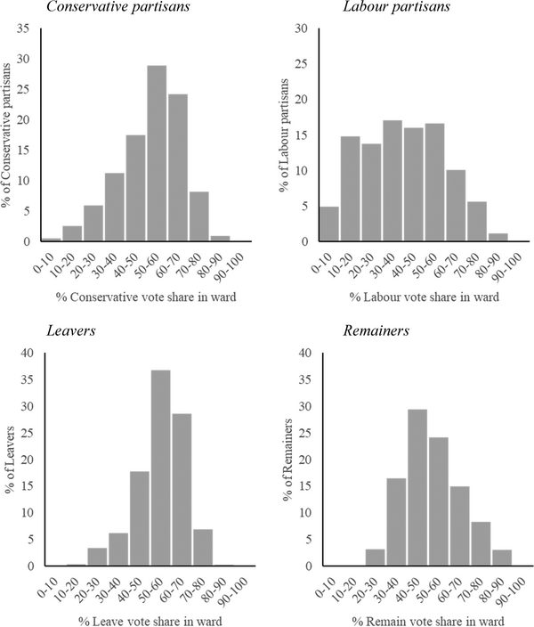
We measure neighbourhood homogeneity as the percentage of people who voted for the same party/side as the respondent's identity in the respondent's ward. Figure 1 shows the distribution of this proportion for the four identity groups. Although Leavers and Conservatives are somewhat more likely to live in areas with high numbers of co-partisans, there is variation for all four groups meaning that some of our respondents are in areas with mostly people like them, but others find themselves as part of a small minority political group within their local area. It is interesting to compare these numbers with US data. Bishop (Reference Bishop2009, p. 305) showed that 48 per cent of voters in the US lived in ‘landslide counties’ (those decided by 20 or more percentage points) in 2008. Almost exactly the same number of British voters, 46 per cent, in our data lived in a similarly defined ‘landslide’ Brexit ward, in which either Leave or Remain were 20 points ahead.

Figure 1. Distribution of respondents by level of ward homogeneity. Note: Ward vote shares are estimates of 2019 General Election vote in England and Wales and the 2016 EU referendum vote in Britain by ward. Proportions of people are based on their group identities.
Control variables
In the models of affective polarization, we include social characteristics to control for social sorting and political values to control for ideological sorting. The social characteristics are age, gender, education, race, occupational social class, household income, trade union membership, housing tenure and religiosity (see Appendix 4 for more details). Political values are measured using four scales based on a battery of 24 items. The first two value scales measure people's position on the two main dimensions of political ideology: economic left-right and social conservative-liberal (Evans et al., Reference Evans, Heath and Lalljee1996; Heath et al., Reference Heath, Evans and Martin1994). We also include two other value scales, one measuring national pride (Heath et al., Reference Heath, Taylor, Brook and Park1999) and another measuring support for the EU. Full details are in online Appendix 5.
Analysis
We first model how actual geographical homogeneity affects perceptions of homogeneity using hierarchical linear models with random effects for a ward.Footnote 5 These models predict perceptions on the −2 to +2 scale, where +2 is the perception that ‘almost all people’ in the local area vote the same way as the respondent and −2 is ‘almost all people’ vote the opposite way to the respondent. We predict these perceptions using the share of fellow voters in that person's ward plus controls for ideology. The models are in Appendix 6. Figure 2 shows the marginal effects of ward homogeneity, for each identity group separately, on perceptions of whether someone's local area is similar to them politically. Positive coefficients thus indicate that perceptions of greater numbers of co-identifiers in the local area are associated with actual greater numbers of people in the ward who share the respondent's political convictions.
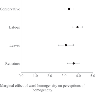
Figure 2. Marginal effects of party and Brexit homogeneity at the ward level on perceptions of local area group homogeneity by group. Note: Perceptions of homogeneity and ward homogeneity are calculated with reference to the respondent's identity. Ward vote shares are estimates of 2016 EU referendum vote in Britain and 2019 General Election vote in England and Wales by ward. Perceptions are scored on a 5 point scale using a question which asks ‘how do you think most people in your local area voted in’ the 2019 General Election or 2016 EU referendum: −2 corresponds to ‘almost all’ people voted differently to the respondent, −1 to ‘most people’ voted differently, 0 to an ‘equal mixture’, +1 to ‘most people’ voted the same way and +2 to ‘almost all’ people voted the same way. All models control for four ideological scales. Full models are in the online Appendix 6.
For all four identities, there are very strong effects of local geographical homogeneity on perceptions. For example, the coefficient from the model for Conservative partisans is 3.34. That means that Conservative partisans who live in a ward with 80 per cent fellow Conservative voters score two points higher on the perceptions scale than Conservatives who live in a ward with 20 per cent fellow Conservative voters. This is the difference between saying ‘most people vote Conservative’ and ‘most people vote Labour’. People are clearly aware of the political make-up of their local area: partisans know whether their neighbours vote the same way as they do. But does this mean that the political makeup of the neighbourhood influences people's affinity for their political in-group and animosity towards their political out-group?
The next step is to estimate whether the political makeup of someone's neighbourhood is associated with affective polarization. Figure 3 thus shows the marginal effects of models predicting the various measures of affective polarization using ward political homogeneity (see Appendix 7 for the full results) plus controls for social characteristics and ideology. We model affective polarization separately for each identity group: Conservative partisans, Labour partisans, Leavers and Remainers. For partisans, we predict the thermometer difference between the in-group and out-group party, the thermometer difference between in-group partisans and out-group partisans, in-group strength, in-group affinity (or positive partisanship), out-group animosity (or negative partisanship) and, finally, out-group prejudice. For Brexit identities, we have measures of the thermometer difference between the in-group and out-group, in-group strength, in-group affinity and out-group prejudice. As mentioned, the out-group for Leavers is Remainers and the out-group for Remainers is Leavers. Similarly, the out-group for Conservative supporters is Labour supporters and the out-group for Labour supporters is Conservative supporters.
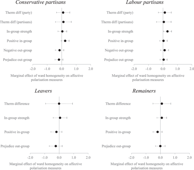
Figure 3. Marginal effects of ward party and Brexit homogeneity on affective polarization. Note: We calculate ward homogeneity with reference to the respondent's identity. Ward vote shares are estimates of 2016 EU referendum vote in Britain and 2019 General Election vote in England and Wales by ward. Thermometer differences are scaled to run from 0–5, in-group strength is scored 1–4 and all other measures are 5-point scales. In all cases, higher scores indicate greater affective polarization. All models control for demographics (gender; age; educational qualifications; race; occupational class; household income quintiles; union membership; housing tenure and religiosity) and four ideological scales. Full models are in the online Appendix 7.
As Figure 3 shows, out of 20 effects, only one (in-group strength of Labour partisans) is statistically significant at the 5 per cent level. Moreover, seven of the 20 coefficients are negative. Since the coefficients can be straightforwardly interpreted as the effect on the scales of moving from a ward that has zero per cent in-group voters to a ward that has 100 per cent in-group voters, it is clear that even if we were to accept the point estimates at face value, the magnitude of any effect is extremely small. We thus find no evidence of an association between local area political homogeneity and affective polarization for either of the political identities.Footnote 6 Affective polarization, measured in any way, was not associated with geographical political homogeneity in Britain in 2021. Moreover, as we show in the next section, this result appears to be very robust.
Robustness tests
First, we look at whether our results are robust to the conditional effects of geographical homogeneity. One might imagine that certain types of people in certain types of area are more affected by local political homogeneity. In terms of the type of people, the most important characteristic is how long someone has lived in the area as it seems plausible that neighbourhood effects only kick in after people have lived in the neighbourhood for a while. Appendix 8 shows models which interact length of residence with homogeneity. We find no evidence that people who have lived in a neighbourhood for a longer time are more likely to polarize if their local area is politically homogenous. In terms of type of area, we look at population density. Here one might imagine that people living in more isolated wards that cover larger areas, normally in the countryside, may be more affected by their neighbours’ preferences. Appendix 9 shows that this is not the case: people who live in areas which differ by population density are no more, or less, likely to be affected by their area's political homogeneity.
Second, our results are robust to different estimates of neighbourhood homogeneity, including at smaller and larger levels of aggregation. In Appendix 10, we replicate all the analysis for partisans using known local election results (these are elections for local councils in which candidates still run on party labels and typically feature the same range of parties as at general elections) by ward and for Brexit identifiers with a subset of known results by ward collected by the BBC.Footnote 7 The results are essentially unchanged. In Appendix 11, we replicate all our analysis with estimates of vote share at the Census Output Area level. These are hyper-local areas that nest within wards and only contain around 130 households. The main results do not change. In Appendix 12, we also replicate all our analysis for partisans with actual votes cast at the 2019 General Election at the parliamentary constituency level. There are 650 constituencies, so these are roughly 10–15 times larger than wards. Again, the main results do not change.
Finally, one might think that the effect of area homogeneity on affective polarization may not be linear. It could be that people become more affectively polarized when they live in areas that contain almost all similar partisans. For example, someone's local area may need to pass a ‘tipping point’ in its makeup to produce affective polarization. Equally, it could be that people become more affectively polarized when they live in politically homogeneous neighbourhoods that do not align with their own partisanship (for example, a Labour supporter living in an area in which there are very few other Labour supporters). We find no evidence for either process. Appendix 13 shows vote share in quintiles as a predictor of affective polarization: no levels of political homogeneity, whether very low or very high, appear to correlate more heavily with polarization.
Conclusion
It seems intuitive that the political makeup of people's local area should affect their attitudes towards political in-groups and out-groups (Bishop, Reference Bishop2009; Lelkes & Westwood, Reference Lelkes and Westwood2017; Sobolewska & Ford, Reference Sobolewska and Ford2020). Yet in the first direct study of geographical homogeneity and affective polarization, we find no association between the two. People clearly recognize that their area is more or less politically homogenous, but that homogeneity is not associated with affective polarization for either of the identities we examine. Why not?
One explanation is that our design is not causal. It could be that there are causal effects of geographical homogeneity on polarization that do not produce an association. We cannot rule that out, given our cross-sectional data. Nonetheless, it seems unlikely that a process by which people become more polarized if they live in a more homogenous area would not leave some trace of a correlation in aggregate. This is especially the case since any reverse causal relationship by which affectively polarized people sort into more homogenous communities should strengthen, not weaken, the association between affective polarization and homogeneity.
Another criticism may be that this (lack of a) relationship is unique to the British case. Of course, we cannot say for certain that our results will generalize to other countries including the most studied case of the US. Nonetheless, as discussed earlier, geographical sorting in Britain is not vastly different in scale to the US, nor are levels of affective polarization in Britain much different to the US or other Western countries (Gidron et al., Reference Gidron, Adams and Horne2020). Indeed, the predominance of two-party politics in Britain should make it easier to find such an association, as people might find it more straightforward to identify the political makeup of their local area, compared to countries with multiple parties and partisan identities.
Perhaps a more plausible explanation for the null result involves the distinction between living near people and spending time in political discussion with those people. The assumption underlying the theoretical expectation of neighbourhood effects on affective polarization is about contact: people who only talk to people like themselves become more wedded to their own side and more hostile to the other side.Footnote 8 Yet living in an area with more co-partisans does not necessarily mean discussing politics with those people. Abrams and Fiorina (Reference Abrams and Fiorina2012) point out, in their critique of The Big Sort, that very few people discuss politics with their neighbours, indeed few people talk to their neighbours at all. The same is true for Britain (Johnston & Pattie, Reference Johnston and Pattie2006; Pattie & Johnston, Reference Pattie and Johnston1999). It seems likely that occasional superficial interactions within one's neighbours that involve little more than pleasantries may not influence attitudes towards political groups. This is heightened by the fact that few people in Britain, or indeed any country, live in completely politically segregated neighbourhoods. As Johnston and Pattie (Reference Johnston and Pattie2006, p. 124) note, even in an area which is 70 per cent Conservative the chance that three random neighbours will all be Conservatives is still only about a third.
Hence, when examining the homogeneity of people's networks, there is perhaps a need to focus on closer relationships with fewer people. It requires discussion of salient political issues with family and friends to polarize ideological perceptions of the parties (Pattie & Johnston, Reference Pattie and Johnston2016), and it seems logical that this applies to affective polarization as well.Footnote 9 On the one hand, this is reassuring. Any increase in geographical political segregation is less likely to produce political disharmony than one might initially expect. On the other hand, this makes reducing existing polarization more difficult. If the main reinforcing mechanism of networks on affective polarization is political discussion with close friends and family, then it is also harder to think of interventions that could reduce levels of out-group animosity.
Acknowledgements
We would like to thank the anonymous reviewers and the editors of the European Journal of Political Research for their very constructive and helpful comments. We would also like to thank Bert Bakker, Martin Baxter, Florian Foos, Eelco Harteveld, Miguel Pereira, Andres Reiljan, Toni Rodon, Luana Russo, Albert Ward and Anthony Wells for comments on, or help with, earlier versions of the paper.
Conflicts of Interest Statement
The authors declare no conflicts of interest.
Funding
This research was funded by the Economic and Social Research Council (grant number ES/V004360/1).
Data Availability Statement
The replication files for the study can be accessed at https://dataverse.harvard.edu/dataset.xhtml?persistentId=doi:org/10.7910/DVN/SNFRC5
Online Appendix
Additional supporting information may be found in the Online Appendix section at the end of the article:


 Open access