1. Introduction
Income inequality has been at the center of the macroeconomic platform over the past few decades. It has been extensively documented that since the 1980s the US residual wage inequality accounts for a major proportion of its overall wage inequality and tends to increase faster among individuals with higher education (having some college or above).Footnote 1 In this paper, we highlight two key stylized facts:
[Fact 1] Over
 $70\%$
of overall inequality among the highly educated has been due to the residual inequality and about four-fifths of the residual wage inequality driven by wage dispersion within jobs, defined by industry–occupation pairs.Footnote
2
$70\%$
of overall inequality among the highly educated has been due to the residual inequality and about four-fifths of the residual wage inequality driven by wage dispersion within jobs, defined by industry–occupation pairs.Footnote
2
[Fact 2] Over the period of 1990–2018, the rise in the residual wage inequality of the highly educated has been particularly prominent during the early phase of 1993–2001.Footnote 3
Despite its important roles played in rising income inequality, little is known toward understanding the underlying drivers of within-job residual wage inequality, particularly so among the highly educated since the mid-1990s. To address this issue, we construct a novel sorting equilibrium model to explore theoretically several potentially important channels, both the intensive and the extensive margins, and then to quantify their contributions over the decades of 1990 and 2000 with the sharpest rising inequality.
In the higher education group, even if we control for more job characteristics including industry and occupation, about
 $90\%$
of the residual wage inequality remains. By decomposing the residual wage inequality into the between-job and within-job components over all the industry—occupation pairs, we find that the within-job wage inequality accounts for about
$90\%$
of the residual wage inequality remains. By decomposing the residual wage inequality into the between-job and within-job components over all the industry—occupation pairs, we find that the within-job wage inequality accounts for about
 $80\%$
of the residual wage inequality between 1990 and 2000. This suggests that the wage inequality among individuals with higher education is primarily driven by the within-industry/occupation inequality. To explain the aforementioned facts, we construct a sorting equilibrium model where, in addition to different job productivity levels, we consider (i) two extensive margin channels—workers optimally self-select into different jobs and pay positions (performance-pay versus fixed-pay positions) and (ii) an intensive channel—the quality of skill match. The chief purpose of the model is to investigate whether these margins may be important to explain the two facts on within-job inequality we established.
$80\%$
of the residual wage inequality between 1990 and 2000. This suggests that the wage inequality among individuals with higher education is primarily driven by the within-industry/occupation inequality. To explain the aforementioned facts, we construct a sorting equilibrium model where, in addition to different job productivity levels, we consider (i) two extensive margin channels—workers optimally self-select into different jobs and pay positions (performance-pay versus fixed-pay positions) and (ii) an intensive channel—the quality of skill match. The chief purpose of the model is to investigate whether these margins may be important to explain the two facts on within-job inequality we established.
Notably, the performance-pay incidence and match quality margins have direct data measurements. Yet, the sorting margin needs to be backed out upon calibrating the model—because this margin is between jobs, the calibration in general equilibrium is nontrivial due to computation of all job sorting wage cutoffs with the range of wages of each job all endogenously determined.
Workers in the performance-pay position are paid according to how much they contribute, and such payments usually include bonuses, commission, piece rates, and tips. The counterpart to this is the payment of a fixed hourly wage. While the literature has identified a positive wage effect of performance-pay, for example, by Lemieux et al. (Reference Lemieux, MacLeod and Parent2009), we further examine the relation between the within-job wage inequality and the performance-pay incidence and find a significant positive relationship: jobs with higher performance-pay incidence usually have higher wage inequality. This hints at the potential role of the rising performance-pay incidence for widening wage dispersion. We measure job match quality based on the inverse relationship with skill mismatch. We compute the skill mismatch index for each job using workers’ occupation-relevant skill and ability measures from the 1979 National Longitudinal Survey of Youth (NLSY79) and occupation skill requirements from O*NET. Previous work such as Guvenen et al. (Reference Guvenen, Kuruscu, Tanaka and Wiczer2020) identify a negative wage effect of skill mismatch whereby better job match quality is associated with higher compensation, we further show a negative relationship between the skill mismatch index and within-job wage inequality: jobs with lower match quality are paid more equally. Hence, improved match quality may also serve to explain the within-job wage inequality. By conducting regression analysis, we find that increases in performance-pay incidence or match quality raise wage inequality significantly. While the empirical analysis suggests a plausible relationship between the wage inequality of each job and the job characteristics of interests in partial equilibrium, the result might be different in general equilibrium and when interactions between different channels are allowed. In addition, the regression results are silent on the counterfactual scenario, thus limiting the ability to conduct rich policy analysis. This thereby requires a deep structure to discipline the interactions among them.
In our sorting equilibrium framework, workers are heterogeneous in their innate abilities. Each job is associated with different productivity and two payment schemes: performance pay and fixed pay. In a fixed-pay position, a worker earns a pooled wage independent of his/her ability, effort or match quality. In the performance-pay position, a worker’s pay positively depends on his/her contribution to production. A worker in a better-matched job is captured by drawing a higher productivity premium from matching, which leads to a higher wage payment. Higher expected match quality thus plays an important role in position selection and job sorting.
Job-specific disutility is incurred for workers in a performance-pay position to capture monitoring costs. Match quality and the resulting productivity-premium also vary by job. In the sorting equilibrium, workers optimally choose their jobs and positions. Under proper assumptions, we show that equilibrium sorting is positive assortative, with the less talented workers choosing the fixed-pay position and the more talented workers selecting the performance-pay position at different jobs based on job productivity and the expected returns dependent on matching premium.
The within-job wage inequality can then be decomposed into that within the performance-pay position and the differences in the average wage between the performance-pay and the fixed-pay positions. In general, performance-pay income is more dispersed than fixed-pay income. Analytically, in a one-job case, we can establish a positive relationship between the performance-pay incidence and within-job wage inequality when the share of the educated workers in the performance-pay position is not too large. This case is equivalent to a multi-job one under a given sorting outcome. A better technology or higher match quality is shown to amplify the effect of the performance-pay incidence on the within-job and the within-performance-pay inequality but dampens its effect on the within-job and between-position inequality, thereby leading to an ambiguous net impact overall. The relative magnitudes of these effects depend crucially on the degree of complementarity between workers in different positions and their relative employment size. With endogenous sorting across jobs, the resulting cutoff abilities further interact with performance pay and match quality in a complex manner. As a consequence, how various channels affect the within-job wage inequality becomes a quantitative question.
To quantify the roles of the performance-pay incidence, match quality, job productivity, and job sorting played in rising wage inequality, we calibrate the model by matching several of the key job-specific features of wage inequality and employment in the US economy in 2000. To conduct counterfactual–based decomposition exercises, we restore the value of each job-specific factor in 2000 to the corresponding value in 1990 by perturbing the distribution of each variation, while maintaining all the other parameters at their benchmark values. The results indicate that our model can capture most of the changes in within-job wage inequality from 1990 to 2000, with an essentially zero residual component. Our decomposition analysis suggests that changes in performance pay and match quality alone account for around
 $90\%$
of widening within-job wage inequality. Moreover, we find amplifying interactive effect compared with the situation if we either let the performance-pay incidence or match quality take their values in 1990. While sorting makes a modest contribution to the widening inequality, the role of residual job productivity is inconsequential. Since performance pay and match quality are the main drivers, pro-active policy intervention aiming to reduce inequality may be at the expense of less prevalence of performance pay or skill mismatch.
$90\%$
of widening within-job wage inequality. Moreover, we find amplifying interactive effect compared with the situation if we either let the performance-pay incidence or match quality take their values in 1990. While sorting makes a modest contribution to the widening inequality, the role of residual job productivity is inconsequential. Since performance pay and match quality are the main drivers, pro-active policy intervention aiming to reduce inequality may be at the expense of less prevalence of performance pay or skill mismatch.
Intuitively, once match quality is assured and workers are offered with correct incentives by performance pay with better ones selecting performance pay positions, the role played by positive assortative sorting across jobs must diminish as a consequence. Ex ante one cannot tell which type of sorting is strong and the existing literature is silent about this. In this paper, we provide a thorough quantitative contrast between them. Moreover, job-specific productivity alone does not convert to higher output—it must be combined with workers’ ability and the quality of match. Thus, to some degree, it resembles the Solow residual in neoclassical aggregate production—departing from the neoclassical canonical framework; however, within- and cross-job sorting is in play in our paper. The results indicate that upon incorporating performance pay and match quality, residual productivity adds little explanatory power to underlying drivers in the model—a finding granting the paper as an endogenous TFP story.
We also perform similar decomposition exercises based upon, respectively, changes in the rankings of average wages and employment shares from 1990 to 2000. The lion’s share of the contribution (more than
 $85\%$
) to widening within-job inequality comes from jobs whose average earnings rankings change moderately (by 1 or 2) or remain unchanged, where both performance pay and match quality play comparably important roles. For jobs whose employment share rankings remain unchanged, which make up more than half of the changes in the overall within-job inequality, match quality is found to play a greater role than the performance-pay incidence.
$85\%$
) to widening within-job inequality comes from jobs whose average earnings rankings change moderately (by 1 or 2) or remain unchanged, where both performance pay and match quality play comparably important roles. For jobs whose employment share rankings remain unchanged, which make up more than half of the changes in the overall within-job inequality, match quality is found to play a greater role than the performance-pay incidence.
The main takeaway of our paper is that while the within-job wage inequality accounts for about
 $80\%$
of the residual wage inequality between 1990 and 2000, approximately
$80\%$
of the residual wage inequality between 1990 and 2000, approximately
 $90\%$
of such rising dispersion is a consequence of higher performance-pay incidence and improved match quality. Once the extensive margin via performance pay and the intensive margin via match quality are incorporated, job sorting becomes much less important, while residual job productivity is inconsequential throughout for the within-job wage inequality. Policymakers concerning earned income inequality should thus be careful to account for the equity-efficiency tradeoff because the two primary sources of wage dispersions within jobs—performance pay and match quality—are natural in the eyes of production efficiency.
$90\%$
of such rising dispersion is a consequence of higher performance-pay incidence and improved match quality. Once the extensive margin via performance pay and the intensive margin via match quality are incorporated, job sorting becomes much less important, while residual job productivity is inconsequential throughout for the within-job wage inequality. Policymakers concerning earned income inequality should thus be careful to account for the equity-efficiency tradeoff because the two primary sources of wage dispersions within jobs—performance pay and match quality—are natural in the eyes of production efficiency.
1.1 Related literature
Several studies have documented the trend of rising wage inequality since the 1970s (e.g., Piketty and Saez, Reference Piketty and Saez2003; Acemoglu and Autor, Reference Acemoglu and Autor2011). Although one convincing theory claims that skill–biased technology change can account for the rising skill premium (e.g., Juhn et al., Reference Juhn, Murphy and Pierce1993; Krusell et al., Reference Krusell, Ohanian, Ríos-Rull and Violante2000; Acemoglu, Reference Acemoglu2003), Altonji et al. (Reference Altonji, Kahn and Speer2016) argue that earnings differences among college students across majors can be larger than the skill premium between college and high school. In general, the residual wage inequality accounts for most of the overall increased wage inequality (e.g., Katz and Autor, Reference Katz and Autor1999; Lemieux, Reference Lemieux2006).
Recent studies focus on within-industry or within-firm wage inequality. For example, Barth et al. (Reference Barth, Bryson, Davis and Freeman2011) emphasize the role of plant differences within industries and argue that this could explain two-thirds of wage inequality in the United States, whereas Card et al. (Reference Card, Heining and Kline2013) find that plant heterogeneity and assortativeness between plants and workers explain a large part of the increase in wage inequality in West Germany. Additionally, Mueller et al. (Reference Mueller, Ouimet and Simintzi2017) study the skill premium within firms and find that firm growth has increased wage inequality. While Papageorgiou (Reference Papageorgiou2011) highlights the labor markets within firms and concludes that the within-firm part might explain one-eighth to one-third of the increase in wage inequality, Song et al. (Reference Song, Price, Guvenen, Bloom and Von Wachter2019) argue that the between-firm component can explain two-third of the rise in wage inequality. To compare our results with theirs, we note that “within industry” includes both within-firm and between-firm, while “within firm” includes both within-occupation and between-occupation. Thus, there are intersections between within-firm and within industry-occupation, and the between-firm part appears to be the main reason for rising within industry-occupation inequality in our exercise.
There are also a growing number of studies that examine wage inequality between and within occupation (see, e.g., Erosa et al. Reference Erosa, Fuster, Kambourov and Rogerson2024). While Kambourov and Manovskii (Reference Kambourov and Manovskii2009) argue that the variability of productivity shocks in occupations coupled with endogenous occupational mobility could account for most of the increase in within-group wage inequality between the 1970s and mid-1990s, Scotese (Reference Scotese2012) shows that changes in wage dispersion within occupations are quantitatively as important as wage changes between occupations for explaining wage inequality between 1980 and 2000. In a more related study, Akerman et al. (Reference Akerman, Helpman, Itskhoki, Muendler and Redding2013) use Sweden employee–employer data to decompose the residual wage inequality and find that within the sector-occupation component (which we call within jobs) it accounts for a large proportion for both the level and change from 2001 to 2007. We confirm that a similar trend is found using the US data.
Performance pay The literature on performance pay either studies incentives and productivity (e.g., Jensen and Murphy, Reference Jensen and Murphy1990; Lazear, Reference Lazear2000) or explains the racial or gender wage gap through the different performance-pay rates by race or gender (e.g., Heywood and Parent, Reference Heywood and Parent2012; Heywood and Parent, Reference Heywood and Parent2017). Makridis (Reference Makridis2018) finds a positive relationship between the performance-pay incidence and wage premium and shows that longer working hours lead to more on-the-job human capital investment. While his study focuses on the dynamic effects of performance pay on human capital accumulation, our study emphasizes the interactions among performance pay, match quality and sorting within and between jobs. In addition, Makridis and Gittleman (Reference Makridis and Gittleman2022) find that performance-pay jobs adjust compensation more on the intensive margin, for which we concur but our incorporation of the aforementioned interactions produces richer results. Another relevant study is Lemieux et al. (Reference Lemieux, MacLeod and Parent2009), who suggest performance pay as a channel through which the underlying changes in returns to skills are translated into higher wage inequality. They conclude that wages in performance-pay jobs are more sensitive to abilities and that inequality is much higher. While the within-job selection in their work is a partial equilibrium outcome, our general equilibrium framework adds two important features: (i) the wages in the non-performance-pay position affect selections in all the jobs. (ii) sorting across jobs affects within-job sorting. In addition, while they emphasize the monitoring cost on selection, we highlight match quality as another driver affecting sorting both within and between jobs. Furthermore, Wallskog et al. (Reference Wallskog, Bloom, Ohlmacher and Tello-Trillo2024) identifies empirically that the increase of within-firm inequality is mainly driven by adoption of aggressive performance-pay bonus and management schemes, thereby lending support to the channels proposed in our theory.
Quality of skill match The general idea of skill mismatch is that workers that share the same characteristics might have different productivity from the job or machine in or on which they are working. Violante (Reference Violante2002) provides a channel through vintage capital to decompose the residual wage inequality into a worker’s ability dispersion, a machine’s productivity dispersion, and the correlation between them. He argues that this channel could explain most transitory wage inequality and 30% of residual wage inequality. Jovanovic (Reference Jovanovic2014) builds a learning–by–doing model to emphasize the role of matching between employees and employers. Under such a framework, he discusses the roles of improving signal quality and assignment efficiency. Both studies are remotely related due to very different model settings and underlying issues of investigation. Concerning the measurement of match quality, there are two general two approaches: (i) the first is to measure the distance between skill requirement and acquirement based on the scores of skills from NLSY79 and O*NET (e.g., Sanders, Reference Sanders2014; Guvenen et al., Reference Guvenen, Kuruscu, Tanaka and Wiczer2020; Lise and Postel-Vinay, Reference Lise and Postel-Vinay2020); (ii) the second is to measure job relatedness between the field of study in the highest degree and current occupation (e.g., Robst, Reference Robst2007; Arcidiacono, Reference Arcidiacono2004; Ritter and West, Reference Ritter and West2014; Kirkeboen et al., Reference Kirkeboen, Leuven and Mogstad2016). Since the second measurement relies on subjective responses that might be biased depending on unobservable individual characteristics, we elect to use the first approach to construct a skill mismatch index following Guvenen et al. (Reference Guvenen, Kuruscu, Tanaka and Wiczer2020).Footnote 4 Finally, Bandiera et al. (Reference Bandiera, Kotia, Lindenlaub, Moser and Prat2024) study mismatch using internationally comparable microdata. Although the main focus is on meritocracy and income difference across countries, one result in this paper that increase technology, which increases the match return, will increase the wage inequality is consistent with our results that high match probability or quality will increase inequality.
2. Stylized facts
Here, we document several stylized facts on performance-pay incidence, skill mismatch, and wage inequality. First, we show how the performance-pay incidence and skill mismatch index are estimated. Second, we compute wage inequality using different measurements, and decompose it into the between- and within-job components. Third, we examine the relationships between the performance-pay incidence, skill mismatch, and wage inequality across jobs.
Our data are collected from several sources, including the March Current Population Survey (March CPS), Panel Study of Income Dynamics (PSID), 1979 National Longitudinal Survey NLSY79, and O*NET. The March CPS includes the most extended high-frequency data series enumerating labor force participation and earnings in the US economy. The PSID contains detailed information on earnings, including commission, bonuses, piece rates, and tips. In NLSY79, respondents were given an occupational placement test—the Armed Services Vocational Aptitude Battery (ASVAB)—that provides detailed measures of occupation-relevant skills and abilities. In addition, respondents reported various measures of non-cognitive skills, which can reflect a worker’s ability for socially interactive work. Finally, O*NET provides the skill requirements for each occupation.
2.1 Estimation of the performance-pay incidence and skill mismatch index
Industry/occupation classification The Center for Economic Policy Research (CEPR) provides two- and three-digit occupation and industry codes. However, the classification is inconsistent from 1983 to 2018. To address this, we build consistent one-digit industry and occupation codes as in Lemieux et al. (Reference Lemieux, MacLeod and Parent2009). Meanwhile, we build a consistent three-digit code following Dorn (Reference Dorn2009). Finally, the same method is used to group a consistent two-digit code.Footnote 5 To circumvent the mis-classification problem over different years due to changes in the content of either occupation or industry, and the problem of empty cells, we use the one-digit industry and occupation codes and check the inclusion of the two-digit occupation code when there is a potential concern.
Performance-pay incidence Performance pay includes bonuses, commission, and piece-rate payment. A significant challenge is to identify workers in a performance-pay position. The PSID, which has been extensively discussed in the literature, reports the format of the payment that a worker has received in a given year among the three performance pay components. However, for workers without those payments, we cannot distinguish whether they work in fixed-pay positions or do not merit, say, bonuses in that given period. Fortunately, the longitudinal nature of PSID data allows us to track the payment history to examine whether a worker has received any form of performance pay in their current job, providing a much more accurate measure (see Lemieux et al., Reference Lemieux, MacLeod and Parent2009).Footnote 6
Following Lemieux et al. (Reference Lemieux, MacLeod and Parent2009), we estimate performance-pay incidence over time using a linear probability model where we regress the dummy of the performance pay on job (industry by occupation) dummy. Specifically, we construct a performance-pay indicator variable looking at whether a part of a worker’s total compensation includes a variable pay component (bonus, commission, or piece-rate) during the sample period. Naturally, conditional on the job duration, we tend to observe a given job match fewer times at the two ends of the sample period than in the middle of the sample. To solve this end-point problem, we follow their solution involving re-balancing the sample using regression or other methods. In practice, we adjust the measures of the performance-pay incidence over time by estimating a linear probability model in which dummies for calendar years and the number of times the job match is observed are included as regressor. We then compute an adjusted measure of the performance pay incidence by using the distribution of the number of times the job match is observed to its average value for the years 1982 to 2000, which are relatively unaffected by the end-point problem. Finally, we keep both less and highly educated workers in PSID for two reasons. First, the sample size would become too small to run the regression if we only retain highly educated workers. Second, we treat the performance-pay incidence as one of the job characteristics so that it would be better to retain the full sample.Footnote 7
We estimate the performance-pay incidence for 80 jobs separately for the years up to 1990 and 2000. To have a consistent code with skill mismatch, we also group them into 25 jobs. Tables 1 and 2 present the results for 25 jobs and show that performance-pay incidence has increased from 1990 to 2000 in general. The results are similar for 80 jobs, as shown in Tables A.9 and A.10.
Table 1. Incidence of performance-pay for 25 jobs: 1990

Notes: This table presents the estimated performance-pay incidence for the highly educated for 25 jobs for the year 1990, following the approach in Lemieux et al. (Reference Lemieux, MacLeod and Parent2009). Data source: PSID.
Table 2. Incidence of performance-pay for 25 jobs: 2000

Notes: This table presents the estimated performance pay incidence for the highly educated for 25 jobs for the year 2000, following the way in Lemieux et al. (Reference Lemieux, MacLeod and Parent2009). Data source: PSID.
Skill mismatch index We approximate the quality of skill match by the inverse of the skill mismatch index. We compute the skill mismatch index using NLSY79 and O*NET following Guvenen et al. (Reference Guvenen, Kuruscu, Tanaka and Wiczer2020). NLSY79 tracks a nationally representative sample of individuals aged between 14 and 22 years on January 1, 1979. It contains detailed information on the industry and occupation in which each individual worked. All respondents took the ASVAB test at the beginning of the survey. The respondents were also given a behavioral test to elicit their social attitudes (e.g., self-esteem and willingness to engage with others). The ASVAB version taken by NLSY79 respondents had 10 component tests. We focus on the following 4 components of verbal and math abilities, which can be linked to skill counterparts: Word Knowledge, Paragraph Comprehension, Arithmetic Reasoning, and Mathematics Knowledge. The NLSY79 included three attitudinal scales that measure a respondent’s non-cognitive abilities. We use two of these measures as social abilities: the Rotter locus of control and Rosenberg self-esteem scales. Because age differences can affect scores, we equalized the mean and variance of each test score across ages. Similar to PSID, we retain the full sample to ensure that we have a sufficient sample size and capture the job’s characteristics.
O*NET includes information on 974 occupations, which can be mapped to the 292 occupation categories included in NLSY79. For each occupation, O*NET analysts score the importance of the 277 descriptors. We use the 26 descriptors most related to the ASVAB component tests and another 6 descriptors related to social skills.
We aggregate information about workers’ abilities and occupational skill requirements into verbal, math, and social ability following Guvenen et al. (Reference Guvenen, Kuruscu, Tanaka and Wiczer2020). We restate them as follows. First, we convert the O*NET skills into four ASVAB test categories using the relatedness score created by the Defense Manpower Data Center. For each ASVAB category test, we create an O*NET analog by summing the 26 descriptors and weighting them by this relatedness score. Therefore, each occupation yields a set of scores comparable to the ASVAB categories, each a weighted average of the 26 original O*NET descriptors.
Second, we normalize each dimension’s standard deviation to be 1 and reduce these 4 ASVAB categories into 2 composite dimensions—verbal and math—by applying principal component analysis. Similarly, we normalize each dimension of the 6 O*NET descriptors related to social skills standard deviation to be 1 and reduce them to a single dimension.Footnote 8 We convert all six scores (verbal, math, and social worker abilities, and verbal, math, and social occupation requirements) into percentile ranks among individuals or occupations.
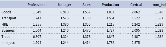
Third, we compute the individual-level mismatch index and then aggregate them into 25 jobs in 1990 and 2000. Tables 3 and 4 show that skill mismatch has decreased in general from 1990 to 2000, that is, the match quality has increased.
Table 3. Skill mismatch index in 1990

Notes: This table presents the average skill mismatch for 25 jobs for the year 1990. “mm_occ” and “mm_ind” represent the average skill mismatch within occupation and industry, respectively. Data source: NLSY79 and ONET, and authors’ calculation.
Table 4. Skill mismat3h index in 2000
Notes: This table presents the average skill mismatch for 25 jobs for the year 1990. “mm_occ” and “mm_ind” represent the average skill mismatch within occupation and industry, respectively. Data source: NLSY79 and ONET, and authors’ calculation.
For robustness check, we also measure the skill mismatch in two alternative ways. First, the current method using total 26 skills in cognitive skills, while as an alternative, one use 6 skills as cognitive skills, representing the minimal level in this category. Figure A.1 presents the comparison in 1990 (left) and 2000 (right) for 2-digit code occupation. It shows that these two measurements are closely related, despite that the values in alternative are slightly higher than the benchmark ones. Second, we measure mismatch by a subjective response on the relatedness between college major and occupation using data from National Survey of College Graduate, then a high relatedness should reflect low skill mismatch.Footnote 9 Figure A.2 compares skill mismatch with the job relatedness and shows a clear-cut negative correlation as expected.
2.2 Measuring wage inequality
We compute the wage inequality using the March CPS where only full-time and full-year workers, defined as those working for at least 40 weeks in a year and 35 hours in a week, and aged between 16 and 65 years. Wages are defined as real hourly earnings. We drop hourly earnings below half the minimum wage in 1982 dollars or higher than USD 1000. The top-coding wage is low in some studies; for example, it is 100 (in 1979 dollars) in Lemieux et al. (Reference Lemieux, MacLeod and Parent2009) and around 180 in Acemoglu and Autor (Reference Acemoglu and Autor2011). Because we focus on highly educated individuals, we do not trim the top incomes by as much.
In the March CPS, the education level is grouped into six categories: primary, high school dropout, high school graduate, some college, college graduate, and post-college. The implied years of schooling are 6, 9, 12, 14, 16, and 18, respectively. Potential experience is then computed as the difference between the year after graduation and age.Footnote
10
The highly educated group includes workers who have some college education and above; the proportion of this group increased from
 $45\%$
in 1983 to
$45\%$
in 1983 to
 $66\%$
in 2018.
$66\%$
in 2018.
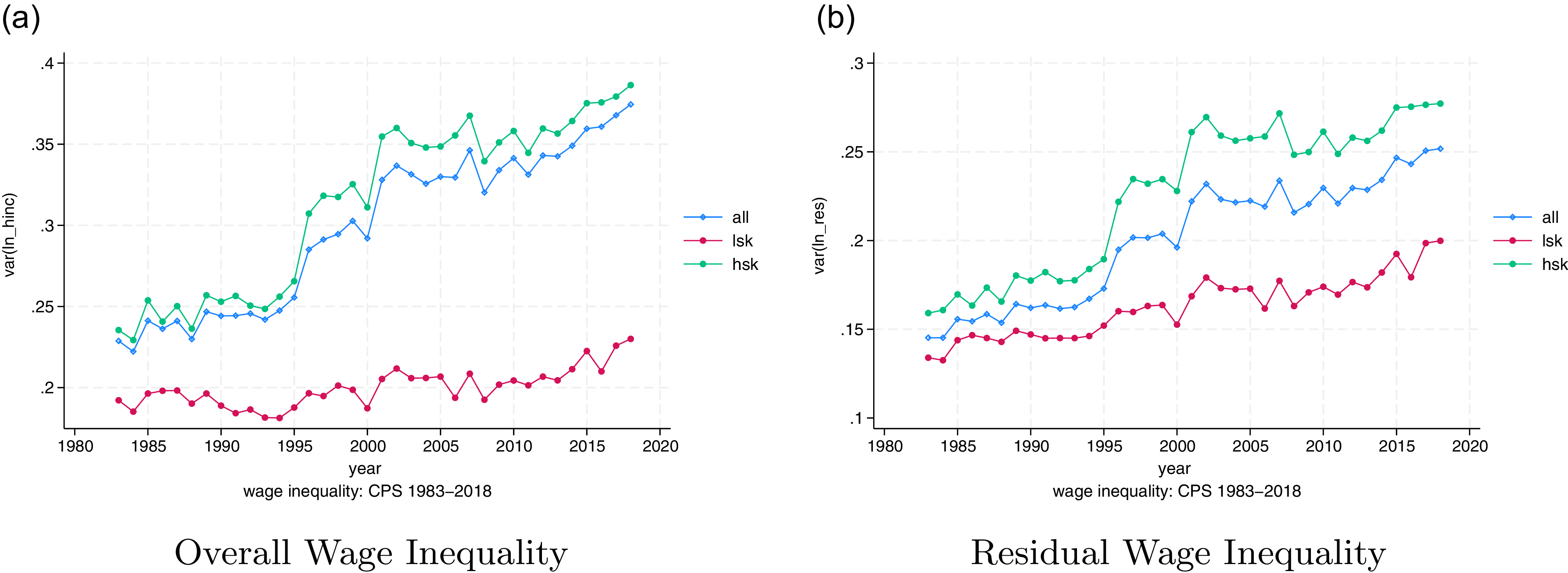
We measure wage inequality as the variance in the logarithm of wage. The left panel of Figure 1 presents the pattern of wage inequality by education group from 1983 to 2018. In general, wage inequality has been increasing since the 1980s among all groups. However, patterns also vary between education groups. Compared with the less educated group, the highly educated group has higher wage inequality and increases faster, especially since the late 1990s.
Following the convention in the literature (e.g., Kambourov and Manovskii, Reference Kambourov and Manovskii2009), we obtain residual wages after controlling for sex, race, experience, and education. The residual wage inequality is then measured as the variance in the residual wages. As shown in the right panel of Figure 1, the highly educated group has higher residual wage inequality which increases faster, especially during 1993–2001. As a robustness check, we calculate the Gini coefficient and 90–10 ratio as well. Figure A.3 shows that both the Gini coefficient and 90–10 ratio exhibit a similar pattern in the highly educated group. In summary, both facts confirm the substantial level of within-group inequality. In addition, the residual wage inequality within the highly educated group exceeds the overall average and increases faster, especially between 1990 and 2000.

Figure 1. Wage inequality by education group.
Notes: In the left (right) panel, the inequality is measured as the variance in the log value of hourly wages (residual wages). In both panels, the blue line represents the inequality for the whole sample (all) and the green line only includes those highly educated or high skilled (hsk). The red line is for the low education group or low skilled (lsk). Data source: March CPS from the CEPR.

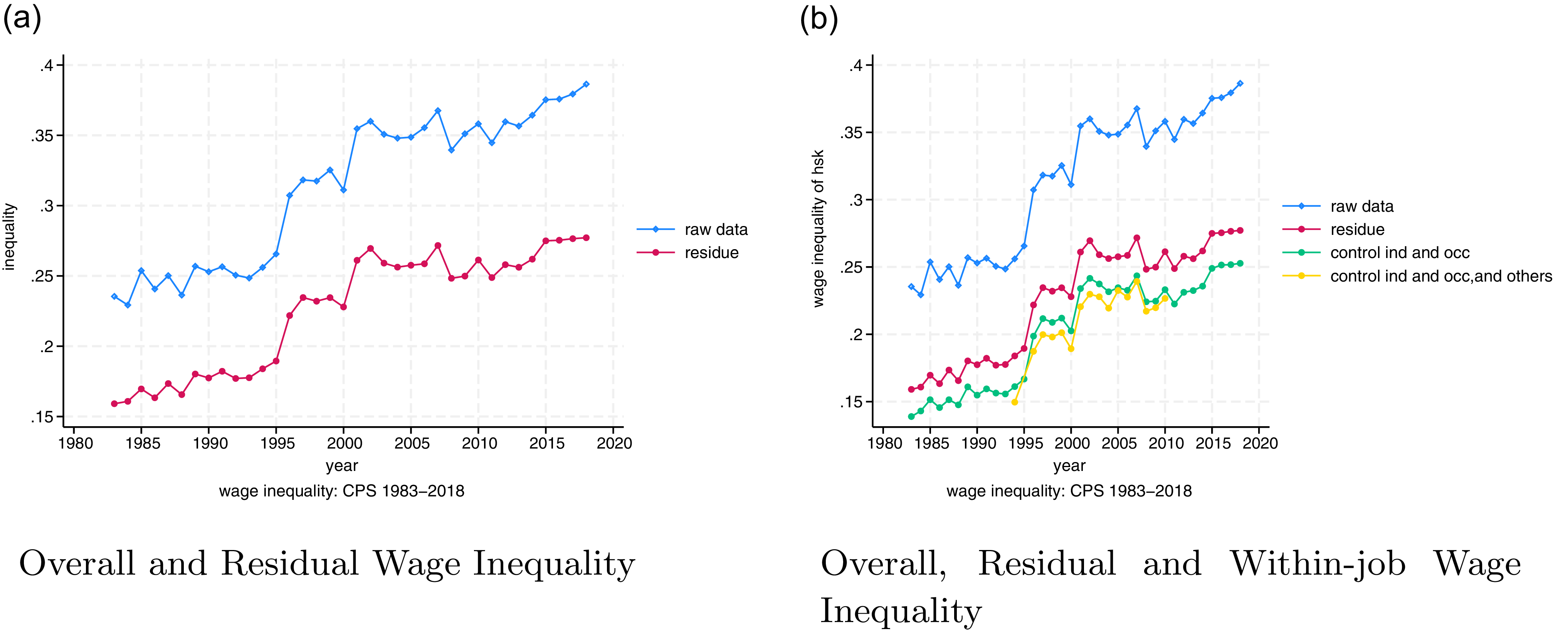
Figure 2. Residual wage inequality of the highly educated.
Notes: In both panels, the inequality is measured among the highly educated. The blue line represents the overall wage inequality. The red line is the residual wage inequality after controlling for only demographic characteristics. The green line is the residual wage inequality after further controlling for occupation and industry. The yellow line is the residual wage inequality after further controlling for location, firm size, and citizenship. Data source: March CPS from the CEPR.
We now examine the inequality within the highly educated group. The left panel of Figure 2 presents the evolution of both the overall and residual wage inequalities. The residual wage inequality accounts for around
 $70\%$
of the overall wage inequality among the highly educated. This proportion is higher than that commonly documented in the literature (e.g., Lemieux, Reference Lemieux2006) for the overall sample comprising individuals of different education levels. The right panel shows the trend of the residual wage inequality when controlling for additional job characteristics, including industry, occupation, location, firm size, and citizenship. Controlling for industry and occupation can only explain
$70\%$
of the overall wage inequality among the highly educated. This proportion is higher than that commonly documented in the literature (e.g., Lemieux, Reference Lemieux2006) for the overall sample comprising individuals of different education levels. The right panel shows the trend of the residual wage inequality when controlling for additional job characteristics, including industry, occupation, location, firm size, and citizenship. Controlling for industry and occupation can only explain
 $10\%$
more of inequality. The result changes little when additional variables, such as location and firm size, are controlled. Thus, the wage inequality within industry and occupation significantly contributes to the residual wage inequality. To consolidate this finding, we decompose the residual wage inequality.
$10\%$
more of inequality. The result changes little when additional variables, such as location and firm size, are controlled. Thus, the wage inequality within industry and occupation significantly contributes to the residual wage inequality. To consolidate this finding, we decompose the residual wage inequality.
2.3 Decomposition of the wage inequality
Here, we decompose both the level and change in residual wage inequality into within- and between-job wage inequalities. A job is defined as an industry-occupation pair. Examples of jobs include sales in the FIRE industry, managers in business, clerical workers in retail/wholesale trade, and production workers in durable/nondurable goods, among others.
Decomposition of the level Suppose there are
 $J$
jobs indexed as
$J$
jobs indexed as
 $j=1,\ldots J$
. In job
$j=1,\ldots J$
. In job
 $j$
, we denote
$j$
, we denote
 $P_{j}$
as the employment share,
$P_{j}$
as the employment share,
 $V_{j}$
as the within-job wage inequality, and
$V_{j}$
as the within-job wage inequality, and
 $E_{j}$
as the average earnings. Then,
$E_{j}$
as the average earnings. Then,
 $\sum _{j}P_{j}V_{j}$
is the average within-job wage inequality weighted by the employment share. Further,
$\sum _{j}P_{j}V_{j}$
is the average within-job wage inequality weighted by the employment share. Further,
 $\sum _{j}P_{j}(\! \ln E_{j}-\sum _{j^{^{\prime }}}P_{j^{^{\prime }}}\ln E_{j^{^{\prime }}})^{2}$
is the weighted average of between-job wage inequality, where
$\sum _{j}P_{j}(\! \ln E_{j}-\sum _{j^{^{\prime }}}P_{j^{^{\prime }}}\ln E_{j^{^{\prime }}})^{2}$
is the weighted average of between-job wage inequality, where
 $\sum _{j^{^{\prime }}}P_{j^{^{\prime }}}\ln E_{j^{^{\prime }}}$
is the weighted average of the logarithm of earnings in the economy. Finally, the overall wage inequality
$\sum _{j^{^{\prime }}}P_{j^{^{\prime }}}\ln E_{j^{^{\prime }}}$
is the weighted average of the logarithm of earnings in the economy. Finally, the overall wage inequality
 $var(\ln E)$
can be decomposed into the between- and within-job components as follows:
$var(\ln E)$
can be decomposed into the between- and within-job components as follows:
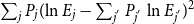
 \begin{equation} var(\! \ln E)=\sum _{j}P_{j}V_{j}+\sum _{j}P_{j}(\! \ln E_{j}-\sum _{j^{^{\prime }}}P_{j^{^{\prime }}}\ln E_{j^{^{\prime }}})^{2}. \end{equation}
The contribution of the within-job wage inequality to the total wage inequality then becomes the ratio of
 $\sum _{j}P_{j}V_{j}$
to
$\sum _{j}P_{j}V_{j}$
to
 $var(\! \ln E)$
.
$var(\! \ln E)$
.
Decomposition of the change We also decompose the changes in the residual wage inequality over time into the various components of interest. In job
 $j$
in year
$j$
in year
 $t,$
let
$t,$
let
 $V_{j,t}$
be the wage inequality,
$V_{j,t}$
be the wage inequality,
 $\ln E_{j,t}$
be the average log earnings,
$\ln E_{j,t}$
be the average log earnings,
 $P_{j,t}$
be the employment share, and
$P_{j,t}$
be the employment share, and
 $\ln E_{t}$
be the average log earnings among all jobs. Then, the change in the within-job wage inequality from
$\ln E_{t}$
be the average log earnings among all jobs. Then, the change in the within-job wage inequality from
 $t$
to
$t$
to
 $t+1$
is
$t+1$
is
 $V_{j,t+1}-V_{j,t}$
, change in the between-job wage inequality is
$V_{j,t+1}-V_{j,t}$
, change in the between-job wage inequality is
 $(\! \ln E_{t+1}-\ln E_{j,t+1})^{2}-(\! \ln E_{t}-\ln E_{j,t})^{2}$
, and change in the employment share is
$(\! \ln E_{t+1}-\ln E_{j,t+1})^{2}-(\! \ln E_{t}-\ln E_{j,t})^{2}$
, and change in the employment share is
 $P_{j,t+1}-P_{j,t}$
. Therefore, the change in the wage inequality between years
$P_{j,t+1}-P_{j,t}$
. Therefore, the change in the wage inequality between years
 $t+1$
and
$t+1$
and
 $t$
,
$t$
,
 $V_{t+1}-V_{t}$
, can be decomposed into four components: the weighted average change in the within-job wage inequality
$V_{t+1}-V_{t}$
, can be decomposed into four components: the weighted average change in the within-job wage inequality
 $\sum _{j=1}^{J}P_{j,t}[V_{j,t+1}-V_{j,t}]$
, the weighted average change in the between-job wage inequality
$\sum _{j=1}^{J}P_{j,t}[V_{j,t+1}-V_{j,t}]$
, the weighted average change in the between-job wage inequality
 $\sum _{j=1}^{J}P_{j,t}[(\! \ln E_{t+1}-\ln E_{j,t+1})^{2}-(\! \ln E_{t}-\ln E_{j,t})^{2}],$
the weighted average change in the employment share
$\sum _{j=1}^{J}P_{j,t}[(\! \ln E_{t+1}-\ln E_{j,t+1})^{2}-(\! \ln E_{t}-\ln E_{j,t})^{2}],$
the weighted average change in the employment share
 $\sum _{j=1}^{J}(P_{j,t+1}-P_{j,t})[V_{j,t}+(\! \ln E_{t}-\ln E_{j,t})^{2}],$
and an interaction term which is the product of the changes in the employment share, and sum of within- and between-job wage inequalities (simply termed as the “interaction” in the decomposition exercise):
$\sum _{j=1}^{J}(P_{j,t+1}-P_{j,t})[V_{j,t}+(\! \ln E_{t}-\ln E_{j,t})^{2}],$
and an interaction term which is the product of the changes in the employment share, and sum of within- and between-job wage inequalities (simply termed as the “interaction” in the decomposition exercise):
 \begin{equation*} \sum _{j=1}^{J}(P_{j,t+1}-P_{j,t})\{(V_{j,t+1}-V_{j,t})+[(\! \ln E_{t+1}-\ln E_{j,t+1})^{2}-(\! \ln E_{t}-\ln E_{j,t})^{2}]\}. \end{equation*}
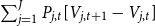
Formally, we decompose the change in wage inequality as follows:
 \begin{align} V_{t+1}-V_{t} & = \sum _{j=1}^{J}P_{j,t}[V_{j,t+1}-V_{j,t}]\nonumber \\ & + \sum _{j=1}^{J}P_{j,t}[(\! \ln E_{t+1}-\ln E_{j,t+1})^{2}-(\! \ln E_{t}-\ln E_{j,t})^{2}]\\ & + \sum _{j=1}^{J}(P_{j,t+1}-P_{j,t})[V_{j,t}+(\! \ln E_{t}-\ln E_{j,t})^{2}]\nonumber \\ & + \sum _{j=1}^{J}(P_{j,t+1}-P_{j,t})\{(V_{j,t+1}-V_{j,t})+[(\! \ln E_{t+1}-\ln E_{j,t+1})^{2}-(\! \ln E_{t}-\ln E_{j,t})^{2}]\}.\nonumber \end{align}
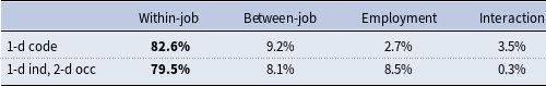
Similarly, each component’s contribution is defined as the ratio of its change to the total change in the residual wage inequality. Table 5 presents the composition of wage inequality from 1990 to 2018. Specifically, the first row shows that the residual wage inequality accounts for a large proportion of the overall wage inequality, which usually exceeds
 $70\%$
for the level and
$70\%$
for the level and
 $50\%$
for the change. More importantly, among the past four decades, the share of changes in residual wage inequality to changes in overall wage inequality is the highest from 1990 to 2000 (
$50\%$
for the change. More importantly, among the past four decades, the share of changes in residual wage inequality to changes in overall wage inequality is the highest from 1990 to 2000 (
 $87.9\%$
). Hence, we focus on 1990 and 2000 in the quantitative analysis. The second row shows that the contribution of the within-job wage inequality is around
$87.9\%$
). Hence, we focus on 1990 and 2000 in the quantitative analysis. The second row shows that the contribution of the within-job wage inequality is around
 $90\%$
for both the level and change under the 1-digit industry and occupation codes. There may be a concern that the significant contribution of the within-job wage inequality is a result of the broad occupation categorization. Hence, we perform a robustness check using the 1-digit (1-d) industry and 2-digit (2-d) occupation codes. As shown in the third row, the contribution of the within-job wage inequality remains sizable, at about
$90\%$
for both the level and change under the 1-digit industry and occupation codes. There may be a concern that the significant contribution of the within-job wage inequality is a result of the broad occupation categorization. Hence, we perform a robustness check using the 1-digit (1-d) industry and 2-digit (2-d) occupation codes. As shown in the third row, the contribution of the within-job wage inequality remains sizable, at about
 $85\%$
for level and above
$85\%$
for level and above
 $80\%$
for change.
$80\%$
for change.
Table 5. How much residual wage inequality accounts for overall inequality
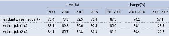
Notes: This table reports how much residual wage inequality accounts for overall inequality by levels or by changes over the previous decade. The first row reports the ratio of residual wage inequality to overall wage inequality. The second row reports the within-job component of residual wage inequality, where the jobs are classified by 1-digit occupations and industries. The third row reports within-job component of residual wage inequality, where the jobs are classified by 1-digit (1-d) industry and 2-digit (2-d) occupation codes. Data source: March CPS.
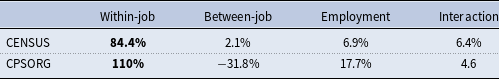
We also perform several other robustness checks. First, Table 6 presents the decomposition results using Census data under the 1-digit codes for the years of 1990 and 2000. The results indicate that the contribution of the within-job component is consistently above
 $80\%$
. In addition, Table A.11 presents the decomposition results using Census data under the 3-digit codes for the years of 1990 and 2000, showing that the contribution of the within-job component exceeds
$80\%$
. In addition, Table A.11 presents the decomposition results using Census data under the 3-digit codes for the years of 1990 and 2000, showing that the contribution of the within-job component exceeds
 $70\%$
. Moreover, Figure A.4 shows that the contribution of the within-job wage inequality is quite large throughout all years. Furthermore, the left panel of Figure A.5 decomposes the overall wage inequality, indicating that the contribution of the within-job wage inequality still exceeds
$70\%$
. Moreover, Figure A.4 shows that the contribution of the within-job wage inequality is quite large throughout all years. Furthermore, the left panel of Figure A.5 decomposes the overall wage inequality, indicating that the contribution of the within-job wage inequality still exceeds
 $75\%$
; and, the right panel that presents the decomposition result using the CPSORG dataset obtains similar findings as well.
$75\%$
; and, the right panel that presents the decomposition result using the CPSORG dataset obtains similar findings as well.
Table 6. Decomposition of residual wage inequality under 1-digit code
Notes: This table computes the contribution of the within-job and between-job inequality to the overall inequality in both 1990 and 2000 using 1-digit industry and occupation code. Data source: CENSUS from CEPR.
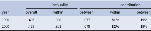
Second, Table 7 reports the contribution of all components between 1990 and 2000 using March CPS, which shows that the within-job significantly dominates other components. Table 8 presents the results using the CENSUS and CPSORG dataset, again showing that the within-job component accounts for the lion’s share. Additionally, Table A.12 summarizes the decomposition results using Census data under the 3-digit industry and occupation codes, where the contributions of the within-job component to the change in the residual wage inequality between 1990 and 2000 also exceed
 $80\%$
.
$80\%$
.
Table 7. Decomposition of the changes in residual wage inequality: March CPS

Notes: This table computes the contribution of within-job, between-job wage inequality, and the employment share interactions to the changes in the residual inequality from 1990 to 2000. The row “1-d code” indicates the one-digit industry and occupation code, “1-d ind, 2-d occ” indicates the one-digit industry and two-digit occupation codes. Data source: March CPS from the CEPR.
Table 8. Decomposition of the changes in residual wage inequality: CENSUS and CPSORG

Notes: This table computes the contribution of the within-job, between-job inequality, employment share and interactions to the changes in the residual wage inequality from 1990 to 2000 under 1-digit industry and occupation code. The row “CENSUS” indicates using data from CENSUS, “CPSORG” indicates using data from CPSORG. Data source: CENSUS and CPSORG from CEPR.
In summary, based on the results in Sections 2.2 and 2.3, we establish two robust stylized facts:
[Fact 1] Over
 $70\%$
of overall inequality among the highly educated has been due to the residual inequality, and about four-fifths of the residual wage inequality is driven by wage dispersion within jobs, defined by industry–occupation pairs.
$70\%$
of overall inequality among the highly educated has been due to the residual inequality, and about four-fifths of the residual wage inequality is driven by wage dispersion within jobs, defined by industry–occupation pairs.
[Fact 2] Over the 1990–2018 period, the rise in the residual wage inequality of the highly educated has been particularly prominent during the early phase of 1993–2001.
2.4 Performance-pay incidence, skill mismatch, and wage inequality
Next, we first explore the correlations between performance-pay incidence, skill mismatch, and within-job wage inequality. Then, we empirically examine how changes in the performance-pay incidence and skill mismatch over time may contribute to the increasing wage inequality. As the datasets are from various sources, throughout the remainder of the study, we classify industries and occupations each into five categories, consistent with the classification in the PSID and NLSY79.Footnote 11
Figure 3 plots the performance-pay incidence against the within-job wage inequality for each of the 25 jobs in 1990 and 2000.Footnote 12 We find a significant positive relationship; that is, jobs with a higher performance-pay incidence usually have higher within-job wage inequality. In Appendix A.2, we also show that the relation is robust to using the same job classification as in Lemieux et al. (Reference Lemieux, MacLeod and Parent2009), containing 52 jobs (Figure A.6). In another robustness check, we plot the performance-pay incidence using the PSID data against wage inequality from the CPSORG dataset in Figure A.7. Furthermore, we try an alternative measurement of performance-pay ratio, defined as the ratio of earnings from performance-pay position to total earnings. Figure A.8 reveals a positive correlation between performance pay and wage inequality under this alternative measurement.
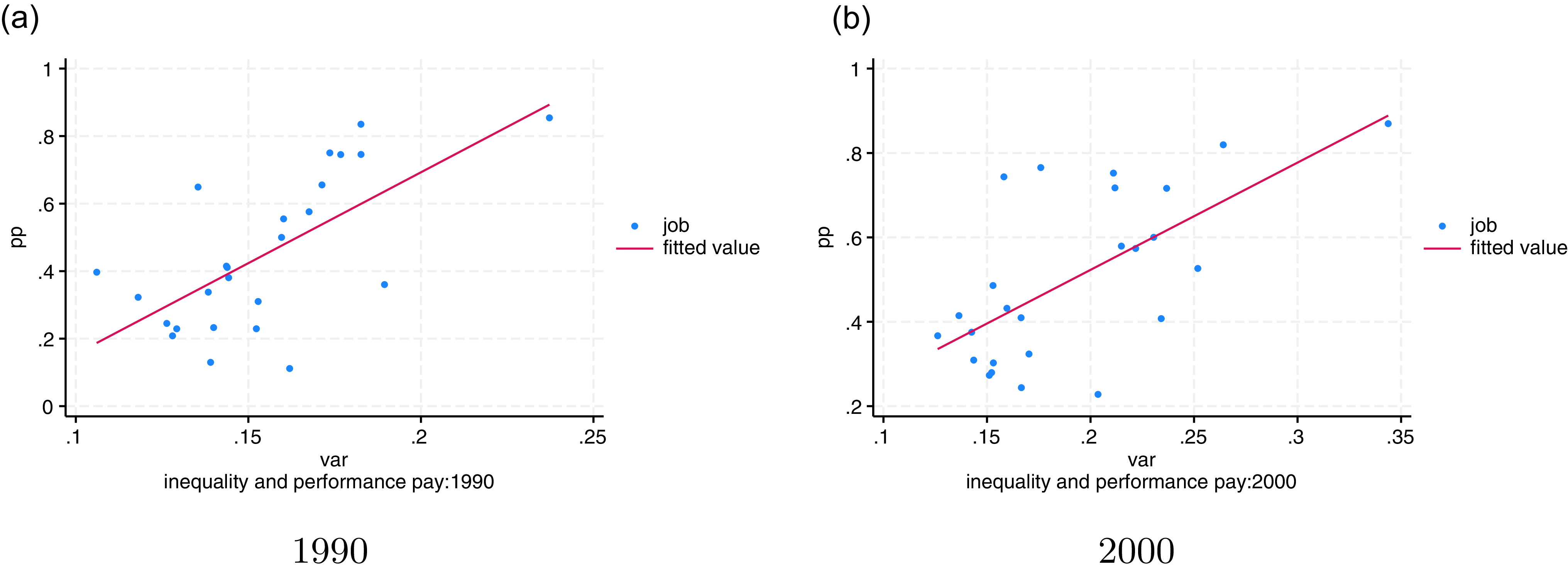
Figure 3. Performance-pay incidence and wage inequality.
Notes: In both panels, each dot represents a job(25 jobs in total). The x-axis is the performance-pay incidence. The y-axis is the within-job wage inequality. The left panel is based on 1990 data and right panel is based on 2000 data. The coefficients in two panels are 5.38 and 2.54, respectively. Data source: PSID and March CPS.
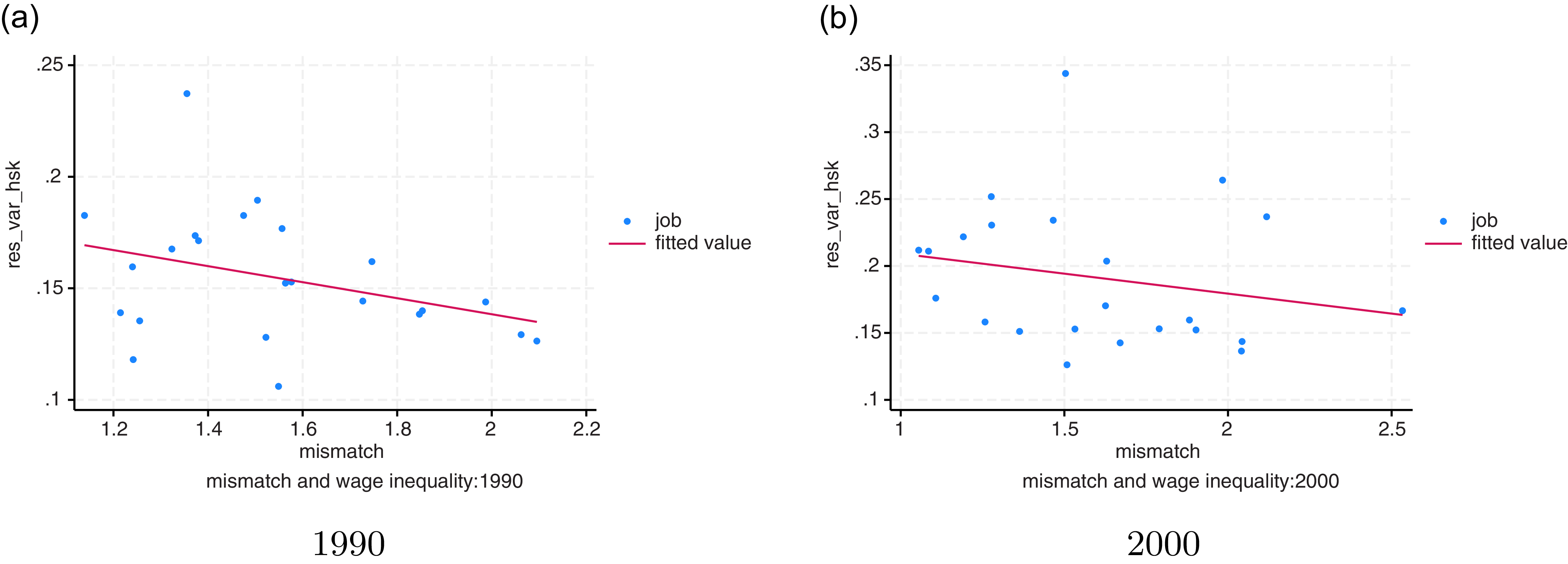
Figure 4. Wage inequality and skill mismatch index.
Notes: In both panels, each dot represents a job(25 jobs in total). The y-axis is the wage inequality. The x-axis is the mismatch index. The left panel is based on 1990 data, and the right panel is based on 2000 data. The coefficients in both panels are
 $-0.03$
. Data source: NLSY79 and March CPS.
$-0.03$
. Data source: NLSY79 and March CPS.
Conversely, we find a negative relationship between the wage inequality and skill mismatch index, as shown in Figure 4. Thus, jobs with better matching quality tend to experience higher wage inequality.
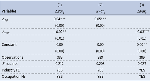
To further explore how performance-pay incidence and match quality increase the rising wage inequality, we first compute the changes in the level of wage inequality, performance-pay incidence, and mismatch index between the current and previous years. We then regress the changes in the wage inequality against the changes in performance-pay incidence and skill mismatch index while controlling for industry and occupation fixed effects:Footnote 13
 \begin{equation*} \triangle var_{ij}=\beta _{1}\Delta _{pp,ij}+\beta _{2}\Delta _{mm,ij}+\beta _{3}i+\beta _{4}j+\epsilon _{ij}. \end{equation*}
Table 9 presents the results. The positive coefficient on the change in performance-pay incidence (
 $\Delta _{pp}$
) implies that rising performance-pay incidence increases the wage inequality. Specifically, if the performance-pay incidence rises by
$\Delta _{pp}$
) implies that rising performance-pay incidence increases the wage inequality. Specifically, if the performance-pay incidence rises by
 $10$
percentage points, the wage inequality rise by
$10$
percentage points, the wage inequality rise by
 $0.4$
percentage points. Similarly, the negative coefficient on the change of skill mismatch index (
$0.4$
percentage points. Similarly, the negative coefficient on the change of skill mismatch index (
 $\Delta _{mm}$
) implies that improving matching quality (lowering mismatch index) increases the wage inequality. The results are robust and significant if we let one or both variables be the regressor. Furthermore, Table A.14 reports significant results when we replace performance-pay incidence with performance-pay ratio.
$\Delta _{mm}$
) implies that improving matching quality (lowering mismatch index) increases the wage inequality. The results are robust and significant if we let one or both variables be the regressor. Furthermore, Table A.14 reports significant results when we replace performance-pay incidence with performance-pay ratio.
Table 9. Performance-pay incidence, skill mismatch and wage inequality

Note:
 $\Delta var_{ij}$
denotes the changes in residual wage inequality between two consecutive years.
$\Delta var_{ij}$
denotes the changes in residual wage inequality between two consecutive years.
 $\Delta _{pp}$
and
$\Delta _{pp}$
and
 $\Delta _{mm}$
is the change in performance-pay incidence and mismatch index between two consecutive years.
$\Delta _{mm}$
is the change in performance-pay incidence and mismatch index between two consecutive years.
Standard errors in parentheses
*
*
* p
 $\lt$
0.01, *
* p
$\lt$
0.01, *
* p
 $\lt$
0.05, * p
$\lt$
0.05, * p
 $\lt$
0.1
$\lt$
0.1
Additionally, we conduct the Firpo–Fortin–Lemieux (FFL) decomposition as in Firpo et al. (Reference Firpo, Fortin and Lemieux2009). Results in Table A.15 and A.16 confirm that performance-pay incidence (mismatch index) is positively (negatively) associated with wage inequality.Footnote 14 Moreover, among other studies, Galindo da Fonseca et al. (Reference Galindo da Fonseca, Gallipoli and Yedid-Levi2020) build a measurement of match quality using vacancy and unemployment information, and find that a high match quality can motivate greater performance pay. We plot performance-pay incidence and match quality using our measurement in Figure A.9 and find they are positively correlated.
Lastly, as the model predicts that the second moment of match quality motivates more performance pay (specified in Section 4), it would be useful to validify this theoretical property. Accordingly, we plot the correlation between the second moment and standard deviation of match quality with performance pay incidence in Figure A.10 and A.11, respectively. The results show that both the second moments and standard deviation of match quality (mismatch) are positively (negatively) correlated with performance pay incidence, conforming with the theoretical prediction.
The empirical analysis presents partial equilibrium results omitting the interactions between different channels and feedback effects via endogenous wage adjustments. Moreover, the results are silent on the counterfactual scenario, thus limiting the ability to conduct rich policy analysis. Hence, this requires a comprehensive structure to discipline the interactions among performance-pay incidence, match quality, and wage inequality, which we explore next.
3. The model
Environment There are
 $J$
jobs available in the economy indexed by
$J$
jobs available in the economy indexed by
 $j=1,2,\ldots J$
. In each job, two types of positions are offered: fixed- (
$j=1,2,\ldots J$
. In each job, two types of positions are offered: fixed- (
 $FP$
) and performance-pay (
$FP$
) and performance-pay (
 $PP$
) positions. Workers are heterogeneous in their innate ability
$PP$
) positions. Workers are heterogeneous in their innate ability
 $a$
, and choose jobs, positions, and efforts to maximize their utilities. Job characteristics and workers’ abilities are both public information.
$a$
, and choose jobs, positions, and efforts to maximize their utilities. Job characteristics and workers’ abilities are both public information.
Performance-pay position A worker’s effective labor supply in the performance-pay position depends on their ability
 $a$
, the job-specific productivity
$a$
, the job-specific productivity
 $A_j$
, an idiosyncratic matching premium
$A_j$
, an idiosyncratic matching premium
 $\eta$
, and their effort level
$\eta$
, and their effort level
 $e$
. Specifically, the effective labor supply is given by
$e$
. Specifically, the effective labor supply is given by
 \begin{equation} h=A_ja\eta e. \end{equation}
The ability
 $a$
follows a Pareto distribution
$a$
follows a Pareto distribution
 $a\sim G(a)=1-(\frac {1}{a})^{\theta _{a}},\ a\geq 1,\theta _{a}\gt 2,$
with the minimum ability normalized to one. We assume
$a\sim G(a)=1-(\frac {1}{a})^{\theta _{a}},\ a\geq 1,\theta _{a}\gt 2,$
with the minimum ability normalized to one. We assume
 $\theta _{a}\gt 2$
to guarantee finite variance, which is essential for studying wage inequality measured by the variance in log wages. To capture the idea of the quality of skill match, we assume that each worker draws an idiosyncratic matching premium from a job-specific Pareto distribution
$\theta _{a}\gt 2$
to guarantee finite variance, which is essential for studying wage inequality measured by the variance in log wages. To capture the idea of the quality of skill match, we assume that each worker draws an idiosyncratic matching premium from a job-specific Pareto distribution
 $\eta \sim F(\eta )=1-(\frac {\underline {\eta _{j}}}{\eta })^{\theta _{sj}}$
defined over
$\eta \sim F(\eta )=1-(\frac {\underline {\eta _{j}}}{\eta })^{\theta _{sj}}$
defined over
 $[\underline {\eta _{j}},\infty )$
, where
$[\underline {\eta _{j}},\infty )$
, where
 $\theta _{sj}\gt 2$
is the inverse of the tail parameter that captures the dispersion of the matching premium in job
$\theta _{sj}\gt 2$
is the inverse of the tail parameter that captures the dispersion of the matching premium in job
 $j$
.
$j$
.
We assume that abilities and the matching premium are distributed independently. Thus, the total effective labor supply in the performance-pay position of job
 $j$
is:
$j$
is:
 \begin{equation} H_{jP}=\int _{a\in D_{jP}}\int _{\eta }h_{jp}(a,\eta )dF_{j}(\eta )dG(a), \end{equation}
where
 $D_{jP}$
is the ability domain for workers, and
$D_{jP}$
is the ability domain for workers, and
 $h_{jp}(a,\eta )$
is the effective labor supply from a worker of ability
$h_{jp}(a,\eta )$
is the effective labor supply from a worker of ability
 $a$
and matching premium
$a$
and matching premium
 $\eta$
.
$\eta$
.
Fixed-pay position A worker’s effective labor supply in the fixed-pay position depends neither on the innate ability nor effort level. It is assumed to be only linear in the job-specific productivity. Precisely, in job
 $j$
, the effective labor supply from a worker in the fixed-pay position is
$j$
, the effective labor supply from a worker in the fixed-pay position is
 $A_{j}$
. Thus, the total effective labor supply in the fixed-pay position of job
$A_{j}$
. Thus, the total effective labor supply in the fixed-pay position of job
 $j$
is
$j$
is
 $H_{jF}=A_{j}N_{jF}$
, where
$H_{jF}=A_{j}N_{jF}$
, where
 $N_{jF}$
is the employment level in the fixed-pay position of job
$N_{jF}$
is the employment level in the fixed-pay position of job
 $j$
.
$j$
.
Production and payment The production function in job
 $j$
is a constant elasticity of substitution (CES) aggregator of the effective labor supply from the performance- and fixed-pay positions. Specifically, the output of job
$j$
is a constant elasticity of substitution (CES) aggregator of the effective labor supply from the performance- and fixed-pay positions. Specifically, the output of job
 $j$
is given by the following:
$j$
is given by the following:
 \begin{equation} Y_{j}=\left [\alpha _{j}H_{jF}^{\gamma }+(1-\alpha _{j})H_{jP}^{\gamma }\right ]^{\frac {1}{\gamma }},\ \gamma \lt 1, \end{equation}
where
 $\frac {1}{1-\gamma }$
is the elasticity of substitution between the labor supply from the two positions—they are substitutes (complementary) if
$\frac {1}{1-\gamma }$
is the elasticity of substitution between the labor supply from the two positions—they are substitutes (complementary) if
 $\gamma \gt 0$
(
$\gamma \gt 0$
(
 $\gamma \lt 0$
);
$\gamma \lt 0$
);
 $\alpha _{j}$
is job specific to reflect the intensity of the fixed-pay position in each job.
$\alpha _{j}$
is job specific to reflect the intensity of the fixed-pay position in each job.
We denote
 $w$
as the wages that each worker in the fixed-pay position can earn. In each job
$w$
as the wages that each worker in the fixed-pay position can earn. In each job
 $j$
, given wages
$j$
, given wages
 $w$
, the representative firm decides the employment level in the fixed-pay position to maximize the revenue net of the payment to workers in the fixed-pay position. That is,
$w$
, the representative firm decides the employment level in the fixed-pay position to maximize the revenue net of the payment to workers in the fixed-pay position. That is,
 \begin{equation} \max _{N_{jF}}Y_{j}-wN_{jF}. \end{equation}
It is straightforward to show that
 $N_{jF}$
satisfies
$N_{jF}$
satisfies
 $N_{jF}=\frac {\chi _{j}(w)H_{jP}}{A_{j}}$
, where
$N_{jF}=\frac {\chi _{j}(w)H_{jP}}{A_{j}}$
, where
 $\chi _{j}(w)\equiv \left [\frac {(\frac {w}{\alpha _{j}{A_{j}}})^{\frac {\gamma }{1-\gamma }}-\alpha _{j}}{1-\alpha _{j}}\right ]^{-\frac {1}{\gamma }}$
. We show in Appendix D that the total payment to workers at the fixed-pay position,
$\chi _{j}(w)\equiv \left [\frac {(\frac {w}{\alpha _{j}{A_{j}}})^{\frac {\gamma }{1-\gamma }}-\alpha _{j}}{1-\alpha _{j}}\right ]^{-\frac {1}{\gamma }}$
. We show in Appendix D that the total payment to workers at the fixed-pay position,
 $E_{jF}$
, is equivalent to
$E_{jF}$
, is equivalent to
 $E_{jF}=\tilde {\alpha }_{j}(w)\tilde {A}_{j}(w)H_{jP}$
, where
$E_{jF}=\tilde {\alpha }_{j}(w)\tilde {A}_{j}(w)H_{jP}$
, where
 $\tilde {A}_{j}(w)=\left [\alpha _{j}\chi _{j}(w)^{\gamma }+(1-\alpha _{j})\right ]^{\frac {1}{\gamma }}$
, and
$\tilde {A}_{j}(w)=\left [\alpha _{j}\chi _{j}(w)^{\gamma }+(1-\alpha _{j})\right ]^{\frac {1}{\gamma }}$
, and
 $\tilde {\alpha }_{j}(w)=\frac {\alpha _{j}\chi _{j}(w)^{\gamma }}{\alpha _{j}\chi _{j}(w)^{\gamma }+(1-\alpha _{j})}$
. We also show in Appendix D that the total output can be expressed as
$\tilde {\alpha }_{j}(w)=\frac {\alpha _{j}\chi _{j}(w)^{\gamma }}{\alpha _{j}\chi _{j}(w)^{\gamma }+(1-\alpha _{j})}$
. We also show in Appendix D that the total output can be expressed as
 $Y_{j}=\tilde {A}_{j}(w)H_{jP}$
. Therefore, the residual profit is
$Y_{j}=\tilde {A}_{j}(w)H_{jP}$
. Therefore, the residual profit is
 $R_{jP}=(1-\tilde {\alpha }_{j}(w))\tilde {A}_{j}(w)H_{jP}$
.
$R_{jP}=(1-\tilde {\alpha }_{j}(w))\tilde {A}_{j}(w)H_{jP}$
.
While the fixed-pay workers are paid at a pooled wage, performance-pay workers’ payments crucially depend on their contribution to production. Given fixed-pay workers, the production function is linear in human capital in the performance-pay position. Hence, a worker’s contribution to the firm is linear in her human capital. Then, the simplest way to model the payment scheme is that the firm and workers in the performance-pay position share the residual profit. We assume that workers’ bargaining power is
 $\mu$
. Therefore, the total payment to workers in the performance-pay position is
$\mu$
. Therefore, the total payment to workers in the performance-pay position is
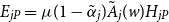 $E_{jP}=\mu (1-\tilde {\alpha }_{j})\tilde {A}_{j}(w)H_{jP}$
, while the payment to a worker of ability
$E_{jP}=\mu (1-\tilde {\alpha }_{j})\tilde {A}_{j}(w)H_{jP}$
, while the payment to a worker of ability
 $a$
and matching premium
$a$
and matching premium
 $\eta$
in the performance-pay position is
$\eta$
in the performance-pay position is
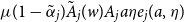 $\mu (1-\tilde {\alpha }_{j})\tilde {A}_{j}(w)A_{j}a\eta e_{j}(a,\eta )$
.
$\mu (1-\tilde {\alpha }_{j})\tilde {A}_{j}(w)A_{j}a\eta e_{j}(a,\eta )$
.
Workers A worker’s utility is assumed to positively depend on their consumption
 $c$
and negatively depend on their effort level
$c$
and negatively depend on their effort level
 $e$
. In addition, workers in the performance-pay position suffer from the job-specific dis-utility of being monitored.Footnote
15
We further assume that a worker’s utility function is linear in consumption and quadratic in the effort level. Specifically, a worker’s utility function from working in the performance-pay position of job
$e$
. In addition, workers in the performance-pay position suffer from the job-specific dis-utility of being monitored.Footnote
15
We further assume that a worker’s utility function is linear in consumption and quadratic in the effort level. Specifically, a worker’s utility function from working in the performance-pay position of job
 $j$
takes the following form:
$j$
takes the following form:
 \begin{equation} U_{j}^{P}=\max _{e}\quad \mu (1-\tilde {\alpha }_{j})\tilde {A}_{j}A_{j}a\eta e-\frac {1}{2}be^{2}-M_{j}, \end{equation}
where
 $b$
measures the degree of dis-utility on effort.
$b$
measures the degree of dis-utility on effort.
 $M_{j}$
is the dis-utility incurred from working in job
$M_{j}$
is the dis-utility incurred from working in job
 $j$
.
$j$
.
Workers make decisions on jobs, positions, and efforts. Figure 5 summarizes the timeline of the worker’s decision. Workers choose the job and position before the realization of the matching premium. Conversely, the optimal effort level is chosen after workers observe the outcome of the matching premium.
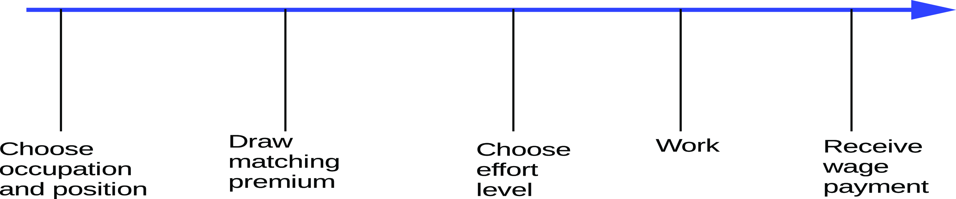
Figure 5. Timeline.
Note: This figure summarizes the timeline for a representative worker in the model economy.
Thus, the ex ante expected utility from working in the performance-pay position of job
 $j$
for a worker of ability
$j$
for a worker of ability
 $a$
is
$a$
is
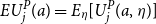 $EU_{j}^{P}(a)=E_{\eta }[U_{j}^{P}(a,\eta )]$
.
$EU_{j}^{P}(a)=E_{\eta }[U_{j}^{P}(a,\eta )]$
.
Workers in the fixed-pay position always exert the minimum effort since their pay is independent of their effort level. Thus, a worker’s payoff from the fixed-pay position can be expressed as follows:
 \begin{equation} U^{F}=w-\frac {b}{2}\underline {e}^{2}. \end{equation}
Finally, a worker chooses the job and position that delivers the highest expected utility:
 \begin{equation} EV(a)=\underset {j}{\max }\{{\max }\{U^{F},EU_{j}^{P}(a)\}\}. \end{equation}
Thus, the fixed-pay position is chosen by a worker of ability
 $a$
if
$a$
if
 $U^{F}\gt \underset {j}{\max }\{EU_{j}^{P}(a)\}$
. Otherwise, a worker of ability
$U^{F}\gt \underset {j}{\max }\{EU_{j}^{P}(a)\}$
. Otherwise, a worker of ability
 $a$
chooses the performance-pay position in a job given by
$a$
chooses the performance-pay position in a job given by
 $j^{\ast }(a)=\arg \underset {j}{\max }\{EU_{j}^{P}(a)\}.$
Two remarks are in order before turning to theoretical results. First, by focusing on the production side, we assume that all goods are perfect substitutes. While this implicitly assumes away the effects of demand shifts and relative price changes on labor and wage inequality, such simplification is not as vulnerable because we focus on highly education labor only. Second, to guarantee positive demand for all jobs or no empty job, we assume a supermodularity condition (as specified in Proposition10 below). Therefore, all jobs will be perfectly sorted according to workers’ abilities.
4. Theoretical analysis
4.1 Equilibrium
Given the job-specific characteristics
 $\{A_{j},\alpha _{j},M_{j},\theta _{sj},\underline {\eta _{j}}\}$
, a sorting equilibrium is described by the wage rate
$\{A_{j},\alpha _{j},M_{j},\theta _{sj},\underline {\eta _{j}}\}$
, a sorting equilibrium is described by the wage rate
 $w$
, effort
$w$
, effort
 $e$
, and job choice (
$e$
, and job choice (
 $j^{\ast }(a)$
) and position (F or P), employment in the fixed-pay position
$j^{\ast }(a)$
) and position (F or P), employment in the fixed-pay position
 $N_{jF}$
, and effective labor supply in performance-pay position
$N_{jF}$
, and effective labor supply in performance-pay position
 $H_{jP}$
, such that:
$H_{jP}$
, such that:
-
1. Given the wage rate
 $w$
, workers optimally choose jobs (
$j^{\ast }(a)$
) and positions (F or p) as in Equation (9).
$w$
, workers optimally choose jobs (
$j^{\ast }(a)$
) and positions (F or p) as in Equation (9). -
2. Given the wage rate
$w$
, workers’ effort
$e$
solve problems in Equation (7). -
3. Given the wage rate
$w$
and job and position choices, the effective labor supply from the performance-pay position
$H_{jP}$
is determined in Equation (4). -
4. Given the wage rate
$w$
and effective labor supply from the performance-pay position
$H_{jP}$
, firms decide employment in the fixed-pay position
$N_{jF}$
to maximize profits in Equation (6) -
5. The wage rate
$w$
clears the labor market, such that:where domain
\begin{equation*} \sum _{j}\int _{a\in \{D_{jF}\cup D_{jP}\}}dG(a)=1, \end{equation*}
$D_{jP}$
and
$D_{jF}$
are the ability domains for workers in performance and fixed-pay positions, respectively, and the total labor force is normalized to 1.


4.2 Analytical results
Next, we solve the worker’s decision in a backward fashion:
-
• (Stage 2) We first solve the effort exerted by a worker of ability
$a$
given that the performance-pay position has been chosen and matching premium draw has been realized. -
• (Stage 1) We then move backward to determine whether this worker would select a performance-pay position and, if so, which job they would take.

Specifically, in Stage 2, a worker of ability
 $a$
in the performance-pay position of job
$a$
in the performance-pay position of job
 $j$
, after realizing the productivity premium
$j$
, after realizing the productivity premium
 $\eta$
, chooses the effort to maximize their utility shown in equation (7). Consumption
$\eta$
, chooses the effort to maximize their utility shown in equation (7). Consumption
 $c_{j}$
equals the wage income:
$c_{j}$
equals the wage income:
 $c_{j}=\mu (1-\tilde {\alpha }_{j})\tilde {A}_{j}A_{j}a\eta e$
. Thus, the resulting effort level is
$c_{j}=\mu (1-\tilde {\alpha }_{j})\tilde {A}_{j}A_{j}a\eta e$
. Thus, the resulting effort level is
 $e_{j}(a,\eta )=\mu (1-\tilde {\alpha }_{j})\tilde {A}_{j}A_{j}a\eta /b$
.
$e_{j}(a,\eta )=\mu (1-\tilde {\alpha }_{j})\tilde {A}_{j}A_{j}a\eta /b$
.
Substituting in the aforementioned effort level, a worker’s effective labor supply is:
 \begin{equation*} h_{jp}(a,\eta )=\frac {\mu (1-\tilde {\alpha }_{j})\tilde {A}_{j}[A_{j}a\eta ]^{2}}{b} \end{equation*}
and the ex post utility from working in job
 $j$
can be derived as
$j$
can be derived as
 \begin{equation*} U_{j}^{P}(a \, ; \, \eta )=\frac {1}{2b}((1-\tilde {\alpha }_{j})\tilde {A}_{j}A_{j}\eta \mu a)^{2}-M_{j}. \end{equation*}
In stage 1, before the realization of the matching premium draw, the decision to select the performance-pay position depends on the expected utility:
 \begin{equation} EU_{j}^{P}(a)\equiv E_{\eta }[U_{j}^{P}(a,\eta )]=\tilde {C}_{j}a^{2}-M_{j}, \end{equation}
where
 $\tilde {C}_{j}=\frac {1}{2b}((1-\tilde {\alpha }_{j})\tilde {A}_{j}A_{j}\mu )^{2}E_{j}(\eta ^{2})$
and
$\tilde {C}_{j}=\frac {1}{2b}((1-\tilde {\alpha }_{j})\tilde {A}_{j}A_{j}\mu )^{2}E_{j}(\eta ^{2})$
and
 \begin{equation} E_{j}(\eta ^{2})=\frac {\theta _{sj}}{\theta _{sj}-2}(\underline {\eta _{j}})^{2}. \end{equation}
Because this second moment
 $E_{j}(\eta ^{2})$
term enters the expected utility from the performance-pay position, we can conveniently use this to measure the match quality in job
$E_{j}(\eta ^{2})$
term enters the expected utility from the performance-pay position, we can conveniently use this to measure the match quality in job
 $j$
. Our result shows that match quality positively depends on both the job-specific minimum matching premium
$j$
. Our result shows that match quality positively depends on both the job-specific minimum matching premium
 $\underline {\eta _{j}}$
and its dispersion measured by the tail parameter
$\underline {\eta _{j}}$
and its dispersion measured by the tail parameter
 $1/\theta _{sj}$
. Recall that
$1/\theta _{sj}$
. Recall that
 $j^{\ast }(a)$
denotes the job in which a worker of ability
$j^{\ast }(a)$
denotes the job in which a worker of ability
 $a$
gains the highest expected utility from the performance-pay position. Thus, the performance-pay position in job
$a$
gains the highest expected utility from the performance-pay position. Thus, the performance-pay position in job
 $j^{\ast }(a)$
is selected by a worker of ability
$j^{\ast }(a)$
is selected by a worker of ability
 $a$
if and only if
$a$
if and only if
 $EU_{j^{\ast }(a)}^{P}(a)\gt U^{F}$
.
$EU_{j^{\ast }(a)}^{P}(a)\gt U^{F}$
.
In summary, the two extensive margins—selection into a performance-pay position and job sorting captured by
 $j^{\ast }(a)$
—are interconnected, depending crucially on the worker’s ability
$j^{\ast }(a)$
—are interconnected, depending crucially on the worker’s ability
 $a$
and an intensive margin of the match quality measure
$a$
and an intensive margin of the match quality measure
 $E_{j}(\eta ^{2})$
. In the sorting equilibrium, all margins, in addition to general job productivity, affect the wage dispersion within each job.
$E_{j}(\eta ^{2})$
. In the sorting equilibrium, all margins, in addition to general job productivity, affect the wage dispersion within each job.
4.3 The one-job case
To gain further insight, consider a scenario of only one job with two available positions: fixed pay and performance pay. Here, the sorting channel is eliminated by construction, thereby enabling us to focus on the effect of performance-pay incidence on wage inequality. It is also an interesting benchmark because it is is equivalent to a multi-job one under a given sorting outcome.
The income earned from each position positively depends on the individual’s ability
 $a$
. We denote
$a$
. We denote
 $y(a)$
and
$y(a)$
and
 $z(a)$
as the income of an agent of ability
$z(a)$
as the income of an agent of ability
 $a$
in the performance- and fixed-pay positions, respectively.Footnote
16
As long as
$a$
in the performance- and fixed-pay positions, respectively.Footnote
16
As long as
 $y^{\prime \prime }(a)\gt z^{\prime \prime }(a)$
and
$y^{\prime \prime }(a)\gt z^{\prime \prime }(a)$
and
 $y(\underline {a})\lt z(\underline {a})$
, workers of higher ability work in the performance-pay position. Let
$y(\underline {a})\lt z(\underline {a})$
, workers of higher ability work in the performance-pay position. Let
 $a^{\ast }$
be the cutoff. The income inequality expressed as the variance in income can be obtained as follows:
$a^{\ast }$
be the cutoff. The income inequality expressed as the variance in income can be obtained as follows:
 \begin{equation} VI=\int _{a^{\ast }}^{\bar {a}}y(a)^{2}dG(a)+\int _{\underline {a}}^{a^{\ast }}z(a)^{2}dG(a)-\left [\int _{a^{\ast }}^{\bar {a}}y(a)dG(a)+\int _{\underline {a}}^{a^{\ast }}z(a)dG(a)\right ]^{2} \end{equation}
Denote
 $n_{p}=\int _{a^{\ast }}^{\bar {a}}dG(a)$
; then,
$n_{p}=\int _{a^{\ast }}^{\bar {a}}dG(a)$
; then,
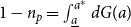 $1-n_{p}=\int _{\underline {a}}^{a^{\ast }}dG(a)$
. In Appendix C, we show that:
$1-n_{p}=\int _{\underline {a}}^{a^{\ast }}dG(a)$
. In Appendix C, we show that:
 \begin{equation} \frac {d(VI)}{dn_{p}}=Var(y(a))-Var(z(a))+(1-2n_{p})\big [E[y(a)]-E[z(a)]\big ]^{2}. \end{equation}
Thus, under normal circumstances, where performance-pay incomes are more dispersed than fixed-pay income (
 $Var(y(a))\gt Var(z(a))$
), we have the following proposition.
$Var(y(a))\gt Var(z(a))$
), we have the following proposition.
Proposition 1.
(Performance-pay Incidence and Wage Inequality) Under
 $Var(y(a))\gt Var(z(a))$
, the overall inequality in the job increases with
$Var(y(a))\gt Var(z(a))$
, the overall inequality in the job increases with
 $n_{p}$
if
$n_{p}$
if
 $n_{p}$
is not too large.
$n_{p}$
is not too large.
Intuitively, how much the performance-pay incidence affects inequality depends on the inequality within the performance-pay position relative to the fixed-pay position, and the gap between the average wages in the two positions. The former effect is expected to be positive, whereas the latter is positive only if
 $n_{p} \lt 1/2$
. If
$n_{p} \lt 1/2$
. If
 $n_{p}$
is not too large, then the former plays a dominant role. We do return to this discussion later under a simplified production function.
$n_{p}$
is not too large, then the former plays a dominant role. We do return to this discussion later under a simplified production function.
Since wage inequality increases with the performance-pay incidence, we next focus on how
 $n_{p}$
is determined within a job. For illustrative purposes, we further assume that the production function takes a Cobb–Douglas form. The firm’s profit maximization problem then becomes
$n_{p}$
is determined within a job. For illustrative purposes, we further assume that the production function takes a Cobb–Douglas form. The firm’s profit maximization problem then becomes
 \begin{equation*} \max \quad \left (AN_{F}\right )^{\alpha }H_{p}^{1-\alpha }-wN_{F}. \end{equation*}
The relationship between wages and employment in the fixed-pay position is
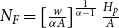 $N_{F}=\left [\frac {w}{\alpha A}\right ]^{\frac {1}{\alpha -1}}\frac {H_{p}}{A}$
.
$N_{F}=\left [\frac {w}{\alpha A}\right ]^{\frac {1}{\alpha -1}}\frac {H_{p}}{A}$
.
Defining
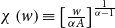 $\chi \left (w\right )\equiv \left [\frac {w}{\alpha A}\right ]^{\frac {1}{\alpha -1}}$
, the total payment to the fixed-pay position can be summarized as
$\chi \left (w\right )\equiv \left [\frac {w}{\alpha A}\right ]^{\frac {1}{\alpha -1}}$
, the total payment to the fixed-pay position can be summarized as
 $\chi \left (w\right )^{\alpha }\alpha H_{p}$
. Following the same notation as in the full-fledged model, we let
$\chi \left (w\right )^{\alpha }\alpha H_{p}$
. Following the same notation as in the full-fledged model, we let
 $\widetilde {A}=\chi \left (w\right )^{\alpha }$
and
$\widetilde {A}=\chi \left (w\right )^{\alpha }$
and
 $\widetilde {\alpha }=\alpha$
. The expected utility from working in the performance-pay position is
$\widetilde {\alpha }=\alpha$
. The expected utility from working in the performance-pay position is
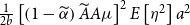 $\frac {1}{2b}\left [\left (1-\widetilde {\alpha }\right )\widetilde {A}A\mu \right ]^{2}E\left [\eta ^{2}\right ]a^{2}$
, and in the fixed-pay position is
$\frac {1}{2b}\left [\left (1-\widetilde {\alpha }\right )\widetilde {A}A\mu \right ]^{2}E\left [\eta ^{2}\right ]a^{2}$
, and in the fixed-pay position is
 $w$
if we normalize the minimum effort level to zero. Thus, a worker chooses the performance-pay position if and only if
$w$
if we normalize the minimum effort level to zero. Thus, a worker chooses the performance-pay position if and only if
 $\frac {1}{2b}\left [\left (1-\widetilde {\alpha }\right )\widetilde {A}A\mu \right ]^{2}E\left [\eta ^{2}\right ]a^{2}\gt w$
.
$\frac {1}{2b}\left [\left (1-\widetilde {\alpha }\right )\widetilde {A}A\mu \right ]^{2}E\left [\eta ^{2}\right ]a^{2}\gt w$
.
In this simple illustration, we also drop the monitoring cost because it is only useful for sorting workers across jobs. Moreover, since
 $\left (1-\widetilde {\alpha }\right )\widetilde {A}A=\left (1-\alpha \right )\left [\frac {w}{\alpha A}\right ]^{\frac {\alpha }{\alpha -1}}A$
, the cutoff ability
$\left (1-\widetilde {\alpha }\right )\widetilde {A}A=\left (1-\alpha \right )\left [\frac {w}{\alpha A}\right ]^{\frac {\alpha }{\alpha -1}}A$
, the cutoff ability
 $a$
can thus be pinned down from
$a$
can thus be pinned down from
 \begin{equation*} \frac {\mu ^{2}}{2b}\left [\left (1-\alpha \right )\left [\frac {w}{\alpha A}\right ]^{\frac {\alpha }{\alpha -1}}A\right ]^{2}E\left [\eta ^{2}\right ]a^{2}=w. \end{equation*}
In addition, the labor market clearing condition can be expressed as follows:
 \begin{equation*} \left [\frac {w}{\alpha A}\right ]^{\frac {1}{\alpha -1}}\frac {H_{p}}{A}=1-a^{-\theta _{a}}, \end{equation*}
where
 $H_{p}=\frac {\mu }{b}\left (1-\alpha \right )^{2}\left [\frac {w}{\alpha A}\right ]^{\frac {2\alpha }{\alpha -1}}A^{2}E\left [\eta ^{2}\right ]\frac {\theta _{a}}{\theta _{a}-2}a^{2-\theta _{a}}$
.
$H_{p}=\frac {\mu }{b}\left (1-\alpha \right )^{2}\left [\frac {w}{\alpha A}\right ]^{\frac {2\alpha }{\alpha -1}}A^{2}E\left [\eta ^{2}\right ]\frac {\theta _{a}}{\theta _{a}-2}a^{2-\theta _{a}}$
.
We can now prove the existence and uniqueness of the solution
 $\left (a,w\right )$
and characterize the impacts of
$\left (a,w\right )$
and characterize the impacts of
 $A$
and
$A$
and
 $E[\eta ^{2}]$
on the equilibrium outcome. To do this, we substitute the cutoff condition into the labor market equilibrium condition to eliminate
$E[\eta ^{2}]$
on the equilibrium outcome. To do this, we substitute the cutoff condition into the labor market equilibrium condition to eliminate
 $E[\eta ^{2}]$
and manipulate it to arrive at the following equation:
$E[\eta ^{2}]$
and manipulate it to arrive at the following equation:
 \begin{equation} \frac {\mu }{2}\frac {\theta _{a}-2}{\theta _{a}}\left (a^{\theta _{a}}-1\right )\left [\frac {w}{A}\right ]^{\frac {\alpha }{1-\alpha }}=\alpha ^{\frac {1}{1-\alpha }}, \end{equation}
which is referred to as the Labor market Equilibrium (LE) locus. Manipulating the cutoff condition, we obtain the following:
 \begin{equation} \frac {\mu ^{2}}{2b}\left (1-\alpha \right )^{2}\left [\frac {1}{\alpha }\right ]^{\frac {2\alpha }{1-\alpha }}AE\left [\eta ^{2}\right ]a^{2}\left [\frac {w}{A}\right ]^{\frac {1+\alpha }{\alpha -1}}=1, \end{equation}
which is referred to as the cutoff ability (CA) locus.
Clearly, LE is increasing in
 $\frac {w}{A}$
and
$\frac {w}{A}$
and
 $a$
but independent of
$a$
but independent of
 $A$
and
$A$
and
 $E[\eta ^{2}]$
. Moreover, CA is decreasing in
$E[\eta ^{2}]$
. Moreover, CA is decreasing in
 $w/A$
but increasing in
$w/A$
but increasing in
 $a$
and
$a$
and
 $A$
. Thus, the LE locus is downward sloping in the
$A$
. Thus, the LE locus is downward sloping in the
 $(a,\frac {w}{A})$
space, whereas the CA locus is upward sloping, as shown in Figure 6. Intuitively, a higher cutoff ability means more workers in the fixed-pay position, thereby leading to lower fixed-pay wages under the labor market equilibrium. Conversely, for the marginal worker to be indifferent, higher fixed-pay wages raise one’s outside options, thus requiring a higher cutoff ability to maintain indifference.
$(a,\frac {w}{A})$
space, whereas the CA locus is upward sloping, as shown in Figure 6. Intuitively, a higher cutoff ability means more workers in the fixed-pay position, thereby leading to lower fixed-pay wages under the labor market equilibrium. Conversely, for the marginal worker to be indifferent, higher fixed-pay wages raise one’s outside options, thus requiring a higher cutoff ability to maintain indifference.
We first study the boundary properties. Recall that
 $a\geq 1$
and
$a\geq 1$
and
 $\theta _{a}\gt 2$
. Consider the LE locus: as
$\theta _{a}\gt 2$
. Consider the LE locus: as
 $a\rightarrow 1$
,
$a\rightarrow 1$
,
 $\frac {w}{A}\rightarrow \infty$
; as
$\frac {w}{A}\rightarrow \infty$
; as
 $a\rightarrow \infty$
,
$a\rightarrow \infty$
,
 $\frac {w}{A}\rightarrow 0$
. Consider the CA locus: as
$\frac {w}{A}\rightarrow 0$
. Consider the CA locus: as
 $a\rightarrow 1$
,
$a\rightarrow 1$
,
 $\frac {w}{A}\rightarrow \left [\frac {w}{A}\right ]_{\min }\equiv \left \{ \frac {\mu ^{2}}{2b}\left (1-\alpha \right )^{2}\left [\frac {1}{\alpha }\right ]^{\frac {2\alpha }{1-\alpha }}AE\left [\eta ^{2}\right ]\right \} ^{\frac {1-\alpha }{1+\alpha }}$
; as
$\frac {w}{A}\rightarrow \left [\frac {w}{A}\right ]_{\min }\equiv \left \{ \frac {\mu ^{2}}{2b}\left (1-\alpha \right )^{2}\left [\frac {1}{\alpha }\right ]^{\frac {2\alpha }{1-\alpha }}AE\left [\eta ^{2}\right ]\right \} ^{\frac {1-\alpha }{1+\alpha }}$
; as
 $a\rightarrow \infty$
,
$a\rightarrow \infty$
,
 $\frac {w}{A}\rightarrow \infty$
. These, together with the slope properties of the two loci, yield the following proposition.
$\frac {w}{A}\rightarrow \infty$
. These, together with the slope properties of the two loci, yield the following proposition.
Proposition 2. (Existence and Uniqueness) For any job, the position cutoff ability and fixed-pay wages are uniquely determined.
Moreover, in the
 $(a,\frac {w}{A})$
space, an increase in either
$(a,\frac {w}{A})$
space, an increase in either
 $A$
or
$A$
or
 $E[\eta ^{2}]$
only shifts the CA locus up, without affecting the LE locus. This leads to a lower
$E[\eta ^{2}]$
only shifts the CA locus up, without affecting the LE locus. This leads to a lower
 $a$
, higher
$a$
, higher
 $\frac {w}{A}$
, and hence, higher
$\frac {w}{A}$
, and hence, higher
 $w$
.
$w$
.
Proposition 3. (Comparative Statics: Wage and Position Selection) For any job, an increase in technology or match quality reduces the position cutoff ability and increases the fixed-pay wages.

Figure 6. Comparative statics in the one-job case.
Notes: The blue curve denotes equation (14) and the red curve denotes equation (15). The left panel shows the existence and uniqueness of the equilibrium outcome in the simple one-job setting. In the right panel, we either double productivity
 $A$
or match quality summarized by
$A$
or match quality summarized by
 $E[\eta ^{2}]$
to evaluate the changes in
$E[\eta ^{2}]$
to evaluate the changes in
 $w/A$
.
$w/A$
.
Figure 6 illustrates the comparative statics from doubling either productivity or match quality (summarized as
 $E(\eta ^{2})$
). Intuitively, technological improvements lead to higher overall productivity and fixed-pay wages. However, these advancements also result in a lower cutoff ability due to the corresponding increase in performance-pay wages. Consequently, the labor supply to the fixed-pay position is lower, leading to a more-than-proportional increase in the fixed-pay wages. Conversely, an increase in match quality raises the reward in the performance-pay position. By complementarity, this also raises the productivity of the fixed-pay workers, and hence, fixed-pay wages.
$E(\eta ^{2})$
). Intuitively, technological improvements lead to higher overall productivity and fixed-pay wages. However, these advancements also result in a lower cutoff ability due to the corresponding increase in performance-pay wages. Consequently, the labor supply to the fixed-pay position is lower, leading to a more-than-proportional increase in the fixed-pay wages. Conversely, an increase in match quality raises the reward in the performance-pay position. By complementarity, this also raises the productivity of the fixed-pay workers, and hence, fixed-pay wages.
We now return to the characterization of the within-job wage inequality in Equation (13). A natural question arises: How do technology and match quality influence the impacts of performance-pay incidence on the overall wage inequality within the job? As shown in Proposition 3, either shift reduces the cutoff ability and raises the fixed-pay wages. While the latter tends to reduce
 $\big [E[y(a)]-E[z(a)]\big ]^{2}$
, the former expands the range of workers in the performance-pay position but suppresses that in the fixed-pay position. Together, these lead to higher
$\big [E[y(a)]-E[z(a)]\big ]^{2}$
, the former expands the range of workers in the performance-pay position but suppresses that in the fixed-pay position. Together, these lead to higher
 $Var(y(a))$
, lower
$Var(y(a))$
, lower
 $Var(z(a))$
, and hence, larger
$Var(z(a))$
, and hence, larger
 $Var(y(a))-Var(z(a))$
. The presence of these channels of endogenous cross-position spillovers is novel. Thus, one may conclude that rising fixed-pay technology amplifies the effect of the performance-pay incidence in the overall within-job wage inequality if
$Var(y(a))-Var(z(a))$
. The presence of these channels of endogenous cross-position spillovers is novel. Thus, one may conclude that rising fixed-pay technology amplifies the effect of the performance-pay incidence in the overall within-job wage inequality if
 $n_{p}$
is not too large. Regarding higher match quality, an additional direct effect widens the performance-pay dispersion
$n_{p}$
is not too large. Regarding higher match quality, an additional direct effect widens the performance-pay dispersion
 $Var(y(a))$
resulting from the heterogeneous premium draws. Thus, while its net impact on the effect of the performance-pay incidence on the overall within-job wage inequality is generally ambiguous, the likelihood of amplifying the effect of the performance-pay incidence on the overall within-job wage inequality is greater than the technology effect. In summary, we have the following proposition.
$Var(y(a))$
resulting from the heterogeneous premium draws. Thus, while its net impact on the effect of the performance-pay incidence on the overall within-job wage inequality is generally ambiguous, the likelihood of amplifying the effect of the performance-pay incidence on the overall within-job wage inequality is greater than the technology effect. In summary, we have the following proposition.
Proposition 4. (Comparative Statics: Inequality) Suppose that
 $Var(y(a))\gt Var(z(a))$
holds and
$Var(y(a))\gt Var(z(a))$
holds and
 $n_{p}$
is not too large. Then, a better technology or higher match quality amplifies the effect of the performance-pay incidence
$n_{p}$
is not too large. Then, a better technology or higher match quality amplifies the effect of the performance-pay incidence
 $n_{p}$
on the within-job and within-performance-pay inequality (
$n_{p}$
on the within-job and within-performance-pay inequality (
 $Var(y(a))$
), but dampens the effect of the performance-pay incidence
$Var(y(a))$
), but dampens the effect of the performance-pay incidence
 $n_{p}$
on the within-job and between-position wage inequality (
$n_{p}$
on the within-job and between-position wage inequality (
 $\big [E[y(a)]-E[z(a)]\big ]^{2}$
), leading to an overall ambiguous net impact.
$\big [E[y(a)]-E[z(a)]\big ]^{2}$
), leading to an overall ambiguous net impact.
We summarize the rich mechanisms underlying the comparative static results presented in Propositions 3 and 4. First, as in standard neoclassical theory, contributions from fixed- and performance-pay workers to production are Pareto complements. Thus, the fixed-pay technology raises the productivity of both fixed- and performance-pay workers. Likewise, match quality enhances the productivity of workers in both positions. Here, the direct effect on its own position should dominate the indirect effect on the other position. Thus, their impacts on the within-job and between-position wage inequality are unambiguous. Second, there is a labor composition effect via changes in the cutoff ability, as in occupational choice models. When the cutoff is lower, more workers are there in the performance-pay position but fewer in the fixed-pay position. This labor composition effect feeds back to affect income in each job via the labor market equilibrium, and subsequently, changes the between-position inequality. Third, because of the changes in the cutoff ability, the range of ability changes, thereby affecting the dispersion of income in both positions. When the cutoff is lower, inequality in the fixed-pay position narrows, whereas that in the performance-pay position widens. Fourth, changes in the cutoff ability also affect the selection of performance-pay workers. When the cutoff is lower, the performance-pay position is less selective, thus reducing the average productivity of performance-pay workers as a whole. In summary, even under this simplified setup, we have four interactive mechanisms: complementarity, labor composition, relative ability dispersion, and performance-pay selectivity.
If we consider a CES production or sorting mechanism across jobs, the comparative static properties regarding the effect of the performance-pay incidence on the overall within-job wage inequality would become even more complicated. While we examine sorting in greater depth in the next subsection, note that CES production enriches the complementarity mechanism, whereas sorting affects the labor composition, relative ability dispersion, and performance-pay selectivity mechanisms. As shown in Figure 7, when the performance- and fixed-pay positions become more complementary (
 $\gamma =-2$
), the elasticity of substitution is
$\gamma =-2$
), the elasticity of substitution is
 $1/(1-\gamma )=1/3$
. The value of the fixed-pay position tends to decrease with both productivity and match quality, as opposed to increasing in the case of the Cobb–Douglas production function. This is because stronger complementarity dampens the negative labor composition effect in the performance-pay positions. This strengthens the positive interactions between match quality and performance-pay incidence, as indicated by the negative relationship between match quality and cutoff ability. Due to all these rich interactions, understanding such impacts thus becomes a quantitative question, which we investigate in Section 5.
$1/(1-\gamma )=1/3$
. The value of the fixed-pay position tends to decrease with both productivity and match quality, as opposed to increasing in the case of the Cobb–Douglas production function. This is because stronger complementarity dampens the negative labor composition effect in the performance-pay positions. This strengthens the positive interactions between match quality and performance-pay incidence, as indicated by the negative relationship between match quality and cutoff ability. Due to all these rich interactions, understanding such impacts thus becomes a quantitative question, which we investigate in Section 5.

Figure 7. Simulation of the one-job case with the CES production function.
Notes: When the performance-pay and fixed-pay positions become more complementary (
 $\gamma =-2$
) as opposed to in the benchmark Cobb–Douglas production function, we re-evaluate how productivity and match quality affect cutoff abilities and wages.
$\gamma =-2$
) as opposed to in the benchmark Cobb–Douglas production function, we re-evaluate how productivity and match quality affect cutoff abilities and wages.
4.4 Positive assortative sorting equilibrium
Here, we return to the full-fledged model. To circumvent the potential issues associated with multiple equilibria in a general setting, we restrict our attention to the case of a monotone job ranking, under which we order
 $n$
such that
$n$
such that
 $\{M_{n}\}$
and
$\{M_{n}\}$
and
 $\{\tilde {C}_{n}\}$
are increasing sequences of
$\{\tilde {C}_{n}\}$
are increasing sequences of
 $n$
.Footnote
17
In this case, we can characterize the sorting equilibrium.
$n$
.Footnote
17
In this case, we can characterize the sorting equilibrium.
We start with the following lemma to show that in the performance-pay position, higher ability workers choose the job of a larger index.
Lemma 5.
If a worker of ability
 $a$
chooses to work in the performance-pay position of job
$a$
chooses to work in the performance-pay position of job
 $k$
, then the workers of ability
$k$
, then the workers of ability
 $a^{\prime }\gt a$
prefer the performance-pay position in any job
$a^{\prime }\gt a$
prefer the performance-pay position in any job
 $n\geq k$
than in job
$n\geq k$
than in job
 $k$
.
$k$
.
We further characterize workers’ preferences over jobs within the performance-pay position in the following lemmas.
Lemma 6.
If
 $\frac {M_{n}-M_{n-1}}{\tilde {C}_{n}-\tilde {C}_{n-1}}$
is increasing in
$\frac {M_{n}-M_{n-1}}{\tilde {C}_{n}-\tilde {C}_{n-1}}$
is increasing in
 $n$
for all
$n$
for all
 $n\gt 1$
, the workers of ability
$n\gt 1$
, the workers of ability
 $a\in \left (\sqrt {\frac {M_{n}-M_{n-1}}{\tilde {C}_{n}-\tilde {C}_{n-1}}},\sqrt {\frac {M_{n+1}-M_{n}}{\tilde {C}_{n+1}-\tilde {C}_{n}}}\right )$
prefer the performance-pay position at job
$a\in \left (\sqrt {\frac {M_{n}-M_{n-1}}{\tilde {C}_{n}-\tilde {C}_{n-1}}},\sqrt {\frac {M_{n+1}-M_{n}}{\tilde {C}_{n+1}-\tilde {C}_{n}}}\right )$
prefer the performance-pay position at job
 $n$
to that at
$n$
to that at
 $n-1$
and
$n-1$
and
 $n+1$
.
$n+1$
.
Lemma 7.
If
 $\frac {M_{n}-M_{n-1}}{\tilde {C}_{n}-\tilde {C}_{n-1}}$
is increasing in
$\frac {M_{n}-M_{n-1}}{\tilde {C}_{n}-\tilde {C}_{n-1}}$
is increasing in
 $n$
for all
$n$
for all
 $n\gt 1$
, when a worker prefers the performance-pay position in job
$n\gt 1$
, when a worker prefers the performance-pay position in job
 $n$
to
$n$
to
 $n-1$
, they also prefer the performance-pay position in job
$n-1$
, they also prefer the performance-pay position in job
 $n$
to any job
$n$
to any job
 $k\lt n-1$
.
$k\lt n-1$
.
Lemma 8.
If
 $\frac {M_{n}-M_{n-1}}{\tilde {C}_{n}-\tilde {C}_{n-1}}$
is increasing in
$\frac {M_{n}-M_{n-1}}{\tilde {C}_{n}-\tilde {C}_{n-1}}$
is increasing in
 $n$
for all
$n$
for all
 $n\gt 1$
, when a worker prefers the performance-pay position in job
$n\gt 1$
, when a worker prefers the performance-pay position in job
 $n$
to
$n$
to
 $n+1$
, they also prefer the performance-pay position in job
$n+1$
, they also prefer the performance-pay position in job
 $n$
to any job
$n$
to any job
 $k\gt n+1$
.
$k\gt n+1$
.
The proof of the above three lemmas can be found in Appendix C. These lemmas together imply that conditional on the performance-pay position, workers of ability
 $a\in \left (\sqrt {\frac {M_{n}-M_{n-1}}{\tilde {C}_{n}-\tilde {C}_{n-1}}},\sqrt {\frac {M_{n+1}-M_{n}}{\tilde {C}_{n+1}-\tilde {C}_{n}}}\right )$
find it optimal to work in job
$a\in \left (\sqrt {\frac {M_{n}-M_{n-1}}{\tilde {C}_{n}-\tilde {C}_{n-1}}},\sqrt {\frac {M_{n+1}-M_{n}}{\tilde {C}_{n+1}-\tilde {C}_{n}}}\right )$
find it optimal to work in job
 $n$
. We can denote
$n$
. We can denote
 $a_{n}^{\ast } \, :\!= \, \sqrt {\frac {M_{n}-M_{n-1}}{\tilde {C}_{n}-\tilde {C}_{n-1}}}$
as the cutoff ability. Thus, we can conclude that workers of ability
$a_{n}^{\ast } \, :\!= \, \sqrt {\frac {M_{n}-M_{n-1}}{\tilde {C}_{n}-\tilde {C}_{n-1}}}$
as the cutoff ability. Thus, we can conclude that workers of ability
 $a\in \lbrack a_{n}^{\ast },a_{n+1}^{\ast })$
prefer the performance-pay position in job
$a\in \lbrack a_{n}^{\ast },a_{n+1}^{\ast })$
prefer the performance-pay position in job
 $n$
than in any other jobs.
$n$
than in any other jobs.
The previous analysis is restricted to workers in the performance-pay position. Next, we explore how workers choose between the performance- and fixed-pay positions.
Lemma 9.
Denote
 $\underline {U}$
as the lowest level of utility, when
$\underline {U}$
as the lowest level of utility, when
 $ \left (\frac {\underline {U}+M_{1}}{\tilde {C}_{1}}\right )^{1/2}\gt \underline {a}$
, workers of ability
$ \left (\frac {\underline {U}+M_{1}}{\tilde {C}_{1}}\right )^{1/2}\gt \underline {a}$
, workers of ability
 $a\in \left [\underline {a},\left (\frac {\underline {U}+M_{1}}{\tilde {C}_{1}}\right )^{1/2}\right )$
choose to work in the fixed-pay position and workers of ability
$a\in \left [\underline {a},\left (\frac {\underline {U}+M_{1}}{\tilde {C}_{1}}\right )^{1/2}\right )$
choose to work in the fixed-pay position and workers of ability
 $a\in \left [\left (\frac {\underline {U}+M_{1}}{\tilde {C}_{1}}\right )^{1/2},a_{2}^{\ast }\right )$
choose to work in the performance-pay position of job 1.
$a\in \left [\left (\frac {\underline {U}+M_{1}}{\tilde {C}_{1}}\right )^{1/2},a_{2}^{\ast }\right )$
choose to work in the performance-pay position of job 1.
Combining all lemmas above yields the following proposition.
Proposition 10. (Positive Assortative Sorting) If
 $\frac {M_{n}-M_{n-1}}{\tilde {C}_{n}-\tilde {C}_{n-1}}$
is increasing in
$\frac {M_{n}-M_{n-1}}{\tilde {C}_{n}-\tilde {C}_{n-1}}$
is increasing in
 $n$
for all
$n$
for all
 $n\gt 1$
, a sorting equilibrium is positive assortative both within and across jobs when
$n\gt 1$
, a sorting equilibrium is positive assortative both within and across jobs when
 $ \left (\frac {\underline {U}+M_{1}}{\tilde {C}_{1}}\right )^{1/2}\gt \underline {a}$
.
$ \left (\frac {\underline {U}+M_{1}}{\tilde {C}_{1}}\right )^{1/2}\gt \underline {a}$
.
-
(i) Sorting across jobs: Workers of ability
$a\in \left (\sqrt {\frac {M_{n}-M_{n-1}}{\tilde {C}_{n}-\tilde {C}_{n-1}}},\sqrt {\frac {M_{n+1}-M_{n}}{\tilde {C}_{n+1}-\tilde {C}_{n}}}\right )$
find it optimal to work in the performance-pay position of job
$n\gt 2$
, whereas the workers of ability
$a\in \left [\left (\frac {\underline {U}+M_{1}}{\tilde {C}_{1}}\right )^{1/2},a_{2}^{\ast }\right )$
choose to work in the performance-pay position of job 1.
-
(ii) Sorting within jobs: Workers of ability
$a\in \left [\underline {a},\left (\frac {\underline {U}+M_{1}}{\tilde {C}_{1}}\right )^{1/2}\right )$
choose to work in the fixed-pay position of any job.


Figure 8. Job and position choice.
Notes: This figure illustrates the distribution of workers over different jobs’ performance-pay and fixed-pay positions based upon their innate abilities. Workers of the lowest abilities work at fixed-pay positions of each job, followed by workers working at performance-pay position of job 1(black), 2(blue), 3(red), 4(green) in an ascending order.
An illustration of job and position choices To illustrate the sorting equilibrium defined above, Figure 8 provides a simple example. Suppose the light blue line is the ability distribution and there are four jobs: 1 (black), 2 (blue), 3 (red), and 4 (green). Hence, there are four cutoff abilities which, shown in the figure, are
 $a_{1}^{*}=2,$
 $a_{2}^{*}=4,$
 $a_{3}^{*}=6$
, and
$a_{3}^{*}=6$
, and
 $a_{4}^{*}=8$
, respectively. The workers work in the fixed-pay position if
$a_{4}^{*}=8$
, respectively. The workers work in the fixed-pay position if
 $a\lt a_{1}^{*}$
and choose the performance-pay position of job
$a\lt a_{1}^{*}$
and choose the performance-pay position of job
 $n$
if
$n$
if
 $a_{n}^{*}\leq a\lt a_{n+1}^{*},n=1,2,3$
. Finally, workers work in the performance-pay position of job
$a_{n}^{*}\leq a\lt a_{n+1}^{*},n=1,2,3$
. Finally, workers work in the performance-pay position of job
 $4$
if
$4$
if
 $a\geq a_{4}^{\ast }$
. Therefore, in each job, some workers are there in the performance-pay position and others in the fixed-pay position.
$a\geq a_{4}^{\ast }$
. Therefore, in each job, some workers are there in the performance-pay position and others in the fixed-pay position.
4.5 Further discussion
While the model delineated above yields useful implications for wage dynamics and income inequality, some model limitations deserve further comments, particularly along the lines of dynamics, other dimensions of firm heterogeneities and the considerations of low-skilled labor, which are now discussed in order.
Dynamics For the sake of simplicity, our equilibrium sorting framework is basically static. In the quantitative exercises to be conducted below, dynamics are, by construction, captured by changes in exogenous variables or parameters. Thus, potential dynamic channels through human capital accumulation and worker relocation are ignored. Should workers be allowed to accumulate human capital, the advancers can enjoy better performance pay and hence wage dispersion is likely to rise. Similar effects occur when workers may relocate to better paid jobs and improve match quality. While the latter case can be largely captured by our job sorting channel, the former may induce greater within-performance-pay inequality, yielding an even stronger role of performance-pay. That is, while the qualitative findings remain unchanged, one may view our computed contribution by performance-pay as a conservative one.
Other Dimensions of Firm Heterogeneity In our model, two key dimensions of firm heterogeneities under considerations are job-specific technologies and monitoring costs. A common dimension considered in the spatial sorting literature is amenity (e.g., see Diamond and Serrato, Reference Diamond and Serrato2025, and papers cited therein). In addition to location-dependent amenity that is beyond the scope of our paper, it may include firm or job-specific amenities. Sockin (Reference Sockin2022) identifies many such amenities and find higher-paying firms offer better amenities and amenities widen cross-firm wage dispersion. In the content of our paper, one may think of such amenities as being related to firm practices and management quality that may affect the design and prevalence of performance-pay contracts. These are qualitatively equivalent to reductions in the monitoring cost within our framework, which would induce higher performance-pay incidence and greater inequality. Of course, some amenities such as workplace environment may directly yield a positive utility. In this case, workers may be satisfied with a lower-paying job in exchange for better job amenity. Because Sockin’s empirical evidence suggests higher-paying firms offer better amenities, this latter channel is unlikely to be quantitatively dominant. As a consequence, our main findings are most likely to prevail.
On Low-Skilled Labor Our paper focuses exclusively on highly educated workers. This is motivated by the fact that the highly educated are the main contributors to wage inequality (Figure 1) and that both performance pay and match quality matters for wage inequality for this group of workers (Figures 3 and 4). On the contrary, these two channels may not play much a role for low-skilled labor. To see this, we present the correlation between performance pay and wage inequality and that between match quality and wage inequality for this group of workers in Figure A.12 and A.13 in the Appendix A.2. Both correlations turn out to be insignificant. That is, wage dispersion within the low-skilled is unlikely to be driven by performance pay or match quality.
5. Quantitative analysis
5.1 Calibration
We calibrate the benchmark model to the US economy in 2000, similar to Section 2.4, focusing on 25 jobs, as observed in the March CPS, PSID, and NLSY79 datasets. In our model, there are four common parameters
 $\left \{ \mu ,\theta _{a},\gamma ,b\right \}$
and five job-specific parameter series
$\left \{ \mu ,\theta _{a},\gamma ,b\right \}$
and five job-specific parameter series
 $\{A_{j},M_{j},\theta _{sj},\underline {\eta _{j}},\alpha _{j}\}_{j=1}^{J}$
. Two parameters can be preset based on the literature or simple targets. One is
$\{A_{j},M_{j},\theta _{sj},\underline {\eta _{j}},\alpha _{j}\}_{j=1}^{J}$
. Two parameters can be preset based on the literature or simple targets. One is
 $\mu$
, which governs workers’ bargaining power in the performance-pay position. This is set to
$\mu$
, which governs workers’ bargaining power in the performance-pay position. This is set to
 $0.54$
by Hall and Milgrom (Reference Hall and Milgrom2008) and
$0.54$
by Hall and Milgrom (Reference Hall and Milgrom2008) and
 $0.72$
by Shimer (Reference Shimer2005), with others choosing lower values such as
$0.72$
by Shimer (Reference Shimer2005), with others choosing lower values such as
 $0.4$
and
$0.4$
and
 $0.5$
. Because we consider only highly educated workers whose bargaining strength is above average, we set
$0.5$
. Because we consider only highly educated workers whose bargaining strength is above average, we set
 $\mu =0.6$
. Another is
$\mu =0.6$
. Another is
 $\theta _{a}$
, the shape parameter of the Pareto distribution for workers’ innate abilities. We set
$\theta _{a}$
, the shape parameter of the Pareto distribution for workers’ innate abilities. We set
 $\theta _{a}=8.0$
so that the 90–10 earnings ratio in our calibrated economy is about 5.
$\theta _{a}=8.0$
so that the 90–10 earnings ratio in our calibrated economy is about 5.
All other parameters are jointly calibrated based on the model. However, each is more closely connected to a primary target. For the crucial parameter of the elasticity of substitution between the efficient labor supply in the production function
 $\gamma$
, as discussed in Section 4.3, we calibrate it to match the overall between-job wage inequality. The calibrated elasticity indicates that workers at different job positions are complementary, and the value of the fixed-pay position and cutoff ability are decreasing in the match quality. Thus, the higher the match quality is, the stronger are sorting incentives for the performance-pay position and job sorting. For the dis-utility parameter from exerting effort
$\gamma$
, as discussed in Section 4.3, we calibrate it to match the overall between-job wage inequality. The calibrated elasticity indicates that workers at different job positions are complementary, and the value of the fixed-pay position and cutoff ability are decreasing in the match quality. Thus, the higher the match quality is, the stronger are sorting incentives for the performance-pay position and job sorting. For the dis-utility parameter from exerting effort
 $b$
, we set it such that the least talented individual in performance-pay position chooses to exert the same effort level as those workers in the fixed-pay position (i.e., the minimum effort:
$b$
, we set it such that the least talented individual in performance-pay position chooses to exert the same effort level as those workers in the fixed-pay position (i.e., the minimum effort:
 $e_{\min }$
). Regarding job-specific monitoring costs
$e_{\min }$
). Regarding job-specific monitoring costs
 $\{M_{j}\}$
, we normalize
$\{M_{j}\}$
, we normalize
 $M_{1}$
to zero and calibrate the remaining
$M_{1}$
to zero and calibrate the remaining
 $M_{j}$
to match the number of workers in the performance-pay position in each job. As
$M_{j}$
to match the number of workers in the performance-pay position in each job. As
 $\{\theta _{sj}\}$
captures the skewness of the matching premium of each job, they are calibrated to minimize the distance between the model-predicted within-job standard deviation of log earnings and their data counterparts. Regarding whether
$\{\theta _{sj}\}$
captures the skewness of the matching premium of each job, they are calibrated to minimize the distance between the model-predicted within-job standard deviation of log earnings and their data counterparts. Regarding whether
 $\underline {\eta _{j}}$
governs the minimum scale of the Pareto distribution of the matching premium, we first establish the following one-to-one mapping between the mismatch index (
$\underline {\eta _{j}}$
governs the minimum scale of the Pareto distribution of the matching premium, we first establish the following one-to-one mapping between the mismatch index (
 $m_{j}$
) measured in Section 2.1 and match quality(
$m_{j}$
) measured in Section 2.1 and match quality(
 $\eta _{j}$
) in job
$\eta _{j}$
) in job
 $j$
:
$j$
:
 \begin{equation*} m_{j}=m_{j0}+\frac {1}{\eta _{j}}. \end{equation*}
If
 $\eta _{j}$
follows a Pareto distribution defined over
$\eta _{j}$
follows a Pareto distribution defined over
 $[\underline {\eta }_{j},\infty )$
with the shape parameter
$[\underline {\eta }_{j},\infty )$
with the shape parameter
 $\theta _{sj}$
, the distribution function of
$\theta _{sj}$
, the distribution function of
 $m_{j}$
is then
$m_{j}$
is then
 \begin{equation*} \tilde {F}(m_{j})=[\underline {\eta }_{j}\cdot (m_{j}-m_{j0})]^{\theta _{sj}}. \end{equation*}
We thus jointly calibrate the job-specific
 $\{\underline {\eta _{j}},m_{j0}\}$
to minimize the distance between the model-predicted mean and standard deviation of the job-specific mismatch index, and their data counterparts.Footnote
18
This enables us to obtain a match quality series using Equation (11). Recall that
$\{\underline {\eta _{j}},m_{j0}\}$
to minimize the distance between the model-predicted mean and standard deviation of the job-specific mismatch index, and their data counterparts.Footnote
18
This enables us to obtain a match quality series using Equation (11). Recall that
 $\alpha _{j}$
is the coefficient on the labor supply from the fixed-pay position in the production function. Thus, it is calibrated to match the performance-pay incidence in each job, which is equivalent to the employment share of workers in the performance-pay position in any job. Finally, turning to job-specific productivity
$\alpha _{j}$
is the coefficient on the labor supply from the fixed-pay position in the production function. Thus, it is calibrated to match the performance-pay incidence in each job, which is equivalent to the employment share of workers in the performance-pay position in any job. Finally, turning to job-specific productivity
 $\left \{ A_{j}\right \}$
, we calibrate
$\left \{ A_{j}\right \}$
, we calibrate
 $A_{1}$
to match the number of workers in the fixed-pay position and then compute
$A_{1}$
to match the number of workers in the fixed-pay position and then compute
 $\{A_{j}\}_{j=2}^{N}$
according to the ratio of average pay in job
$\{A_{j}\}_{j=2}^{N}$
according to the ratio of average pay in job
 $j$
to that in job
$j$
to that in job
 $1$
. Because these parameters are interconnected in the model, they are jointly calibrated to meet the targets by minimizing distance.
$1$
. Because these parameters are interconnected in the model, they are jointly calibrated to meet the targets by minimizing distance.
Table 10 summarizes the parameter values and their targets. While all other target moments are easily understood, we should note that the “performance-pay incidence” target is the performance-pay ratio within each job, whereas the “dist. of workers at performance-pay” target is the number of workers in the performance-pay position across jobs.
Table 10. Benchmark parameterizations

Notes: This table summarizes parameter value in the benchmark economy. The values for some standard parameters are directly obtained from the literature. The remaining parameters are calibrated to match stylized facts in the data.
To facilitate decomposition analysis in the next subsection, we must obtain the job-specific series in 1990 by recalibrating the model to the 1990 data following an identical strategy to the exercise in 2000. Therefore, we re-calibrate the jobs specific parameters (
 $\{A_{j}, \alpha _{j}, M_{j}, \theta _{sj}, \underline {\eta }_{j}\}$
) in 1990 using job-by-job relative wage, performance-pay incidence, distribution of worker at performance-pay, match quality, and within-job inequality measures, while maintaining other common parameters (e.g.,
$\{A_{j}, \alpha _{j}, M_{j}, \theta _{sj}, \underline {\eta }_{j}\}$
) in 1990 using job-by-job relative wage, performance-pay incidence, distribution of worker at performance-pay, match quality, and within-job inequality measures, while maintaining other common parameters (e.g.,
 $b$
or
$b$
or
 $\gamma$
). Figure B.1 presents the parameters in 2000 (benchmark) and Figure B.2 compares the parameters in 1990 and 2000. We find that
$\gamma$
). Figure B.1 presents the parameters in 2000 (benchmark) and Figure B.2 compares the parameters in 1990 and 2000. We find that
 $\alpha$
and
$\alpha$
and
 $M$
have no clear trend, whereas job-specific productivity
$M$
have no clear trend, whereas job-specific productivity
 $A$
has increased and
$A$
has increased and
 $\theta$
has decreased over time.
$\theta$
has decreased over time.
Owing to the strict parameter restriction,Footnote 19 it is not guaranteed that we can exactly match the data counterparts of each job. Nonetheless, as shown in Figure 9, our calibration is quite precise: the model perfectly matches the within-job inequality of each job in 2000; it perfectly matches the inequality in 1990 in all but one job, (Goods, professional).Footnote 20
Table 11. Benchmark inequality: model versus data

Note: The data on each type of wage inequality are computed from the March CPS dataset. Model-implied wage inequality is based on the calibrated parameters summarized in Table 10.

Figure 9. Model fitness in 2000 and 1990.
Note: The x-axis represents job-specific within-job wage inequality computed from the data and the y-axis is the wage inequality within each job computed from the model. Each dot represents a job.
Notably, in our calibration, we have never targeted any aggregate inequality moments. Such untargeted moments can thus be used to test model fit. In Table 11, we report the model-predicted within-job, between-job, and overall wage inequalities as opposed to the data counterpart in 1990 and 2000. As it can be seen, the model matches these untargeted between-job wage and overall wage inequalities reasonably well.
5.2 Decompose the changes in within-job inequality
Next, we further disentangle how the performance-pay incidence, match quality, sorting, and job-specific productivity affect the pattern of within-job wage inequality. Specifically, we conduct a decomposition analysis that changes the values of each job-specific series in 2000 into their respective values in 1990. All other parameters remain their benchmark values. Performance pay channel is governed by monitoring cost
 $\{M_{j}\}$
, match quality channel by
$\{M_{j}\}$
, match quality channel by
 $\{\theta _{sj}\}$
, and productivity by
$\{\theta _{sj}\}$
, and productivity by
 $\{A_{j}\}$
. As sorting is endogenous, in the counterfactual exercise we shut it down by directly setting the sorting result in 1990 to the economy of 2000 (benchmark).
$\{A_{j}\}$
. As sorting is endogenous, in the counterfactual exercise we shut it down by directly setting the sorting result in 1990 to the economy of 2000 (benchmark).
To evaluate the contribution of factor
 $k$
to the changes in inequality from 1990 to 2000 in job
$k$
to the changes in inequality from 1990 to 2000 in job
 $j$
, denoted as
$j$
, denoted as
 $\pi _{k}^{j}$
, we apply the following formula:
$\pi _{k}^{j}$
, we apply the following formula:
 \begin{equation*} \pi _{k}^{j}=\frac {(model_{2000}^{j}-counter_{k}^{j})}{\sum _{k^{^{\prime }}}(model_{2000}^{j}-counter_{k^{^{\prime }}}^{j})} \bigg( \frac {model_{2000}^{j}-model_{1990}^{j}}{data_{2000}^{j}-data_{1990}^{j}} \bigg), \end{equation*}
where
 $model_{1990}^{j}$
and
$model_{1990}^{j}$
and
 $model_{2000}^{j}$
denote the model-predicted inequalities in 1990 and 2000 in job
$model_{2000}^{j}$
denote the model-predicted inequalities in 1990 and 2000 in job
 $j$
, respectively.
$j$
, respectively.
 $data_{1990}^{j}$
and
$data_{1990}^{j}$
and
 $data_{2000}^{j}$
denote the inequality in the data in these two years.
$data_{2000}^{j}$
denote the inequality in the data in these two years.
 $counter_{k}^{j}$
is the inequality obtained from the counterfactual economy, wherein we restore the job-specific factor
$counter_{k}^{j}$
is the inequality obtained from the counterfactual economy, wherein we restore the job-specific factor
 $k$
from their values in 2000 to those in 1990.
$k$
from their values in 2000 to those in 1990.
Overall, we evaluate four contributing factors from the model: the performance-pay incidence, match quality, job-specific productivity, and sorting-induced changes in abilities and employment shares. The fraction that cannot be accounted for in the model is due to “residuals” arising from missing factors, which is small in the benchmark economy.
Finally, the overall contribution of factor
 $k$
, denoted as
$k$
, denoted as
 $\bar {\pi }_{k}$
, is an average of its contribution in each job weighted by the employment share of each job
$\bar {\pi }_{k}$
, is an average of its contribution in each job weighted by the employment share of each job
 \begin{equation} \bar {\pi }_{k}=\frac {\sum _{j}\pi _{k}^{j}N_{j}}{\sum _{k'}\sum _{j}\pi _{k'}^{j}N_{j}}, \end{equation}
where
 $N_{j}$
is the employment share in job
$N_{j}$
is the employment share in job
 $j$
.
$j$
.
Table 12 reports the overall contribution of each channel. The contributions of the performance-pay incidence, match quality, job-specific productivity, and sorting are
 $37.6\%$
,
$37.6\%$
,
 $51.9\%$
,
$51.9\%$
,
 $-0.8\%$
, and
$-0.8\%$
, and
 $9.2\%$
, respectively. Overall, the model mimics the data counterpart fairly well with a nearly zero residual component. The changes in the performance-pay incidence and match quality can capture almost
$9.2\%$
, respectively. Overall, the model mimics the data counterpart fairly well with a nearly zero residual component. The changes in the performance-pay incidence and match quality can capture almost
 $90\%$
of the changes in within-job wage inequality from 1990 to 2000. Finally, the role of general job productivity is inconsequential.
$90\%$
of the changes in within-job wage inequality from 1990 to 2000. Finally, the role of general job productivity is inconsequential.
Table 12. Contribution of each channel

Notes: The contribution of factor
 $k$
in any job is summarized in equation (16). The overall contribution of factor
$k$
in any job is summarized in equation (16). The overall contribution of factor
 $k$
across all the jobs is computed as the average of its contribution in each job weighted by the employment share.
$k$
across all the jobs is computed as the average of its contribution in each job weighted by the employment share.
One may inquire why job sorting or job-specific productivity does not widen within-job inequality by much. On the one hand, once match quality is assured and workers are offered correct incentives by performance pay with better ones sorted into performance-pay positions, the role played by positive assortative sorting across jobs substantially decreases. On the other hand, job-specific productivity resembles Solow residuals in neoclassical aggregate production. Thus, upon incorporating match quality and performance pay, this residual productivity adds little explanatory power to the underlying drivers in the model.
Interactions between performance-pay incidence and match quality One may wonder when both the channel of performance-pay incidence and match quality are incorporated, and whether they tend to reinforce or offset each other. Here, we address this question by either setting both the performance-pay incidence and match quality, or setting one of them to their levels in 1990. As shown in Table 13, where both are set to their levels in 1990, the joint contribution to changes in the overall wage inequality is
 $96.2\%$
. This implies a positive amplification effect between the two channels by
$96.2\%$
. This implies a positive amplification effect between the two channels by
 $6.7\%$
,Footnote
21
which also echoes our findings in Proposition 4.
$6.7\%$
,Footnote
21
which also echoes our findings in Proposition 4.
Table 13. Contribution of performance pay and match quality

Note: We either set one channel or both channels to their values in 1990 and compute the contribution to changes in the wage inequality in each case.
In summary, once the extensive margin via performance pay and intensive margin via match quality are incorporated, the contribution of the remaining extensive margin via job sorting becomes modest, accounting for only less than
 $10\%$
of the rising within-job wage inequality from 1990 to 2000. Moreover, general job productivity—which has been emphasized in most studies—is inconsequential throughout when performance-pay and match quality are considered. Thus, while widening wage inequality may be a concern, it is less warranted if improved matching quality and better incentivized performance-pay contracts are the underlying drivers. It is particularly so because the modest role played by job sorting suggests that typical labor market search frictions are less likely to be the main source of the widening within-job wage inequality. As such, policymakers concerned about wage inequality should recognize the equity-efficiency tradeoffs because these two primary sources of wage dispersions within jobs are natural in the eyes of production efficiency. Our results also offer, on a more micro-structured basis, insights for a better understanding of the main findings in Jovanovic (Reference Jovanovic2014); in an incomplete information world, this improved signaling quality about workers’ true abilities may widen the within-the-group inequality. While improved match quality may be thought of as due partly to more informed signaling, performance-pay contracts may induce better incentives for workers, mitigating informational frictions.
$10\%$
of the rising within-job wage inequality from 1990 to 2000. Moreover, general job productivity—which has been emphasized in most studies—is inconsequential throughout when performance-pay and match quality are considered. Thus, while widening wage inequality may be a concern, it is less warranted if improved matching quality and better incentivized performance-pay contracts are the underlying drivers. It is particularly so because the modest role played by job sorting suggests that typical labor market search frictions are less likely to be the main source of the widening within-job wage inequality. As such, policymakers concerned about wage inequality should recognize the equity-efficiency tradeoffs because these two primary sources of wage dispersions within jobs are natural in the eyes of production efficiency. Our results also offer, on a more micro-structured basis, insights for a better understanding of the main findings in Jovanovic (Reference Jovanovic2014); in an incomplete information world, this improved signaling quality about workers’ true abilities may widen the within-the-group inequality. While improved match quality may be thought of as due partly to more informed signaling, performance-pay contracts may induce better incentives for workers, mitigating informational frictions.
Table 14. Decomposition by industry

Notes: The five industries are (1) Goods (containing durables/non-durables, construction and mining), (2) Transport (transportation and utility), (3) FIRE, (4) Business (business and professional services), and (5) Trade (whole/retail trade and personal services). The contribution of each factor in an industry is the average of its contribution in each job belonging to that industry weighted by the employment share.
5.2.1 Contribution by industry and occupation
To further examine the role of each channel, we have conducted similar decomposition exercises at the industry/occupation level. The contribution of each channel in a given group is computed as the employment-weighted average of the job-level contributions:
 \begin{align*} \bar {\pi }_{k}^{g}=\frac {\sum _{j\in g}\pi _{k}^{j}N_{j}}{\sum _{j\in g}N_{j}} \end{align*}
where
 $j$
denotes the job index that belongs to the group
$j$
denotes the job index that belongs to the group
 $g$
. For brevity, we focus on those with significant deviations in group outcomes from the overall aggregate outcomes. To evaluate the relative importance of each industry/occupation in driving the widening wage inequality, we have also computed the contribution of each industry/occupation to the increase in the overall within-job inequality. The brief algorithm is to first compute the changes in the wage inequality of each job from 1990 to 2000. The changes in wage inequality at the industry (occupation) level are then an employment-weighted average of job-level changes. The contribution of each industry (occupation) is then the fraction of the changes in each industry or occupation for the changes in the overall within-job inequality. The results are reported in Table B.2 and B.3.
$g$
. For brevity, we focus on those with significant deviations in group outcomes from the overall aggregate outcomes. To evaluate the relative importance of each industry/occupation in driving the widening wage inequality, we have also computed the contribution of each industry/occupation to the increase in the overall within-job inequality. The brief algorithm is to first compute the changes in the wage inequality of each job from 1990 to 2000. The changes in wage inequality at the industry (occupation) level are then an employment-weighted average of job-level changes. The contribution of each industry (occupation) is then the fraction of the changes in each industry or occupation for the changes in the overall within-job inequality. The results are reported in Table B.2 and B.3.
Table 14 presents the results of grouping by industry. Match quality is more important than the performance-pay incidence in almost all industries except for the Trade industry, which accounts for approximately
 $21\%$
of the increase in the overall within-job inequality, as shown in Table B.2. The role of match quality is dominant and higher than the average contributions among all industries in the Transport and FIRE industries, which jointly account for another
$21\%$
of the increase in the overall within-job inequality, as shown in Table B.2. The role of match quality is dominant and higher than the average contributions among all industries in the Transport and FIRE industries, which jointly account for another
 $19.3\%$
of the increase in the overall within-job inequality. Conversely, performance-pay incidence in the Trade and Business industries contributes more than the average level among all industries, accounting for approximately
$19.3\%$
of the increase in the overall within-job inequality. Conversely, performance-pay incidence in the Trade and Business industries contributes more than the average level among all industries, accounting for approximately
 $44.7\%$
of the changes in the overall within-job inequality. That is, incentive provision is more crucial for explaining the widening inequality in the Trade and Business industries. The contribution of sorting is relatively larger in the Goods and Transport industries, exceeding
$44.7\%$
of the changes in the overall within-job inequality. That is, incentive provision is more crucial for explaining the widening inequality in the Trade and Business industries. The contribution of sorting is relatively larger in the Goods and Transport industries, exceeding
 $10\%$
.
$10\%$
.
Table 15 presents the results of grouping by occupations. Specifically, in the Clerical occupation, which accounts for
 $21.8\%$
changes in the overall within-job inequality as shown in Table B.3, performance pay is more important than match quality in driving up the wage inequality, Meanwhile, in all remaining occupations, the contribution of match quality is the largest among the different channels. In Manager, Sales, and Production Labor occupations, which together can explain
$21.8\%$
changes in the overall within-job inequality as shown in Table B.3, performance pay is more important than match quality in driving up the wage inequality, Meanwhile, in all remaining occupations, the contribution of match quality is the largest among the different channels. In Manager, Sales, and Production Labor occupations, which together can explain
 $61.2\%$
of the changes in the overall within-job inequality, the contribution of match quality is higher than the average level. In only two occupations, Production Labor and Clerical, the contribution of job sorting exceeds
$61.2\%$
of the changes in the overall within-job inequality, the contribution of match quality is higher than the average level. In only two occupations, Production Labor and Clerical, the contribution of job sorting exceeds
 $10\%$
.
$10\%$
.
Table 15. Decomposition by occupation

Notes: The five occupations are (1) Professional, (2) Manager, (3) Sales, (4) Production/Operative Labor (including craftsmen), and (5) Clerical (including other services). The contribution of each factor in an occupation is the average of its contribution in each job belonging to that occupation weighted by the employment share.
Tables 14 and 15 show that, among all industries and occupations, the Professional occupation is the only category where the model cannot capture a noticeable portion (
 $12.5\%$
) of the widening inequality. In the Goods industry, the residual accounts for a mild
$12.5\%$
) of the widening inequality. In the Goods industry, the residual accounts for a mild
 $6\%$
. Meanwhile, in all other categories, the residual shares are all negligible.
$6\%$
. Meanwhile, in all other categories, the residual shares are all negligible.
5.2.2 Contribution by wage, employment, or inequality rankings
In the benchmark economy, jobs are sorted by average wages. The rankings of jobs may change from 1990 to 2000. In our exercise, being ranked first implies that the job has the lowest average wage among all jobs. Next, we group jobs with similar changes in ranking to examine how the role of each channel varies by category. If the job’s wage bin rises, this job stands at a higher ranking in 2000 than in 1990. That is, there are more jobs with a lower average wage than in 1990. Table 16 presents the decomposition results grouped by wage bin changes.Footnote
22
For jobs whose average earnings rankings rise/drop moderately (by one or two) or remain unchanged, which account for more than
 $85\%$
of changes in the overall within-job inequality as shown in Table B.4, match quality and performance pay jointly contribute to the widening wage inequality. For jobs whose average earnings rankings rise/drop sharply (by three or more), which contribute to approximately
$85\%$
of changes in the overall within-job inequality as shown in Table B.4, match quality and performance pay jointly contribute to the widening wage inequality. For jobs whose average earnings rankings rise/drop sharply (by three or more), which contribute to approximately
 $12\%$
of changes in the within-job inequality, match quality plays a more dominant role with contributions higher than the overall average; meanwhile, performance pay tends to be more important than in other categories.
$12\%$
of changes in the within-job inequality, match quality plays a more dominant role with contributions higher than the overall average; meanwhile, performance pay tends to be more important than in other categories.
Table 16. Decomposition by average wage bin change

Note: We group jobs with similar changes in ranking. If the job’s average wage bin rises, then there are more jobs with a lower average wage than this job in 2000 than in 1990. The contribution of each factor in a category is again the weighted average of its contribution in each job within that category.
Similarly, we can group jobs by the rankings of their employment share; this also changes from 1990 to 2000, with a first-place ranking representing the lowest employment share. We again group jobs with similar changes in ranking. If the job’s employment bin rises, there are more jobs with a lower employment share than the specific job in 2000 than in 1990. Table 17 presents the results grouped by employment bin changes.Footnote
23
For jobs whose employment share rankings rise, which accounts for about
 $15.3\%$
changes in the overall within-job inequality as shown in Table B.5, match quality plays a dominant role. For jobs whose employment share rankings remain unchanged, which comprise more than
$15.3\%$
changes in the overall within-job inequality as shown in Table B.5, match quality plays a dominant role. For jobs whose employment share rankings remain unchanged, which comprise more than
 $50\%$
of contributions to changes in the overall within-job inequality, the dominant role of match quality diminishes. Finally, its role continues to decline for jobs whose employment share rankings fall, where sorting contributes more than
$50\%$
of contributions to changes in the overall within-job inequality, the dominant role of match quality diminishes. Finally, its role continues to decline for jobs whose employment share rankings fall, where sorting contributes more than
 $10\%$
of changes in the within-job inequality.
$10\%$
of changes in the within-job inequality.
Table 17. Decomposition by employment bin change

Note: We group jobs with similar changes in the ranking of the employment share. If the job’s employment bin rises, then there are more jobs with a lower employment share than this job in 2000 than in 1990. The contribution of each factor in a category is again the weighted average of its contribution in each job within that category.
5.2.3 Contribution in selected jobs
Finally, we investigate six selected jobs based on their large earnings and employment shares (see Table B.6 in the Appendix). Match quality contributes more than performance-pay incidence in almost all industries except for the Trade industry, which accounts for about
 $20\%$
of the changes in the overall within-job inequality. In Transport and FIRE industries, which jointly account for another
$20\%$
of the changes in the overall within-job inequality. In Transport and FIRE industries, which jointly account for another
 $20\%$
of the changes in the overall within-job inequality, match quality plays a dominant role. In the Business industry, the contribution of performance-pay incidence is higher than the average level among all industries. At the occupation level, performance-pay incidence is more important than match quality only in the Clerical occupation, which accounts for approximately
$20\%$
of the changes in the overall within-job inequality, match quality plays a dominant role. In the Business industry, the contribution of performance-pay incidence is higher than the average level among all industries. At the occupation level, performance-pay incidence is more important than match quality only in the Clerical occupation, which accounts for approximately
 $22\%$
of the changes in the overall within-job inequality. In Manager, Sales, and Production Labor occupations, which together account for more than
$22\%$
of the changes in the overall within-job inequality. In Manager, Sales, and Production Labor occupations, which together account for more than
 $60\%$
of the changes in the overall within-job inequality, the contribution of match quality is higher than the average level.
$60\%$
of the changes in the overall within-job inequality, the contribution of match quality is higher than the average level.
6. Conclusion
We document that the within-job component accounts for the lion’s share of residual wage inequality, which itself has been the primary source of overall wage inequality. We examine four plausible channels widening within-job wage inequality, and identify match quality and performance pay as the two key drivers. We shed light on the primary source of residual wage inequality within jobs. While widening wage inequality may be a concern, it is less warranted if improved matching and more prevalent performance pay are the underlying drivers.
Some interesting future research avenues arise along these lines. First, the model can be extended to discuss the underlying reasons for skill mismatch. In particular, a worker may be employed in a mismatched job because of search frictions, or the trade-off between personal interests and earnings. Incorporating these underlying reasons, the model can generate richer policy implications. Second, the model can also be extended to include multiple dimension skills to study the effects of multi-tasking on wage inequality. With rising demand for multi-tasking, the dimension of skill requirements expands and that of job specialization declines. While a worker who fits the job or a special task well may have a higher wage, such a highly specialized skill may turn them into a loser both in multi-tasking requirements and in subsequent re-sorting. Thus, within-job wage inequality may change as the requirements for multi-tasking change in different types of jobs.
Acknowledgements
An earlier version of this paper was circulated under the title “Within-job Wage Inequality: Performance Pay and Job Relatedness”, NBER Working Paper 27390. We thank Daniel Parent, Carl Sanders and David Wiczer for sharing their codes and Gaetano Antinolfi, Sangmin Aum, Michele Boldrin, Fatih Guvenen, Tim Lee, Rodolfo Manuelli, B. Ravikumar, Raul Santaeulalia-Llopis, Yongseok Shin, Guillaume Vandenbroucke, and David Wiczer, as well as an editor and two anonymous referees for helpful comments. We have also benefited from comments by participants at the Asian Meeting of the Econometric Society, China Meeting of Econometric Society, Midwest Macroeconomics Meeting, North American Meeting of Econometric Society, QMUL-SUFE Workshop in Economics, and Taipei International Conference on Growth, Trade and Dynamics. Rongsheng Tang is grateful for the financial support from the National Natural Science Foundation of China (Grant No. 72373088).
Supplementary material
The supplementary material for this article can be found at http://doi.org/10.1017/S1365100525100631.