


This paper considers the “risk-weighted expected utility” ( $REU$
) introduced by Lara Buchak (Reference Buchak2013) (formally identical to the “anticipated utility” introduced by John Quiggin (Reference Quiggin1982), but with a normative rather than a descriptive interpretation), which is based on a risk function
$REU$
) introduced by Lara Buchak (Reference Buchak2013) (formally identical to the “anticipated utility” introduced by John Quiggin (Reference Quiggin1982), but with a normative rather than a descriptive interpretation), which is based on a risk function $R$
that is required to be a continuous, strictly increasing function from the unit interval
$R$
that is required to be a continuous, strictly increasing function from the unit interval $\left[ {0,1} \right]$
to itself. Buchak motivates her generalization of risk-neutral expected utility (
$\left[ {0,1} \right]$
to itself. Buchak motivates her generalization of risk-neutral expected utility ( $EU$
) by arguing that means-ends reasoning requires an improvement in any possible outcome of a gamble to contribute positively to its evaluation, but not necessarily in direct proportion to its probability. On her framework, this corresponds to the requirement that
$EU$
) by arguing that means-ends reasoning requires an improvement in any possible outcome of a gamble to contribute positively to its evaluation, but not necessarily in direct proportion to its probability. On her framework, this corresponds to the requirement that $R$
be strictly increasing.
$R$
be strictly increasing.
Buchak notes (Reference Buchak2013: 68–70) that maximin and maximax preferences could be said to be particularly extreme forms of risk sensitivity that can be accommodated in a generalization of this approach by relaxing the requirement that $R$
be continuous and strictly increasing. But she notes that this involves giving up her means-ends understanding of decision theory. Thus, rather than relaxing strict monotonicity, I relax the requirement that the range of this function be the unit interval. I show that when the interval is infinite, the resulting decision rule still has the maximin or maximax property of prioritizing the best or worst outcome over all others. I observe that the resulting rule is interestingly different in other ways, but satisfies more of the axioms of her representation theorem than the classic maximin and maximax rules, as well as others I call “leximin” and “leximax”.
$R$
be continuous and strictly increasing. But she notes that this involves giving up her means-ends understanding of decision theory. Thus, rather than relaxing strict monotonicity, I relax the requirement that the range of this function be the unit interval. I show that when the interval is infinite, the resulting decision rule still has the maximin or maximax property of prioritizing the best or worst outcome over all others. I observe that the resulting rule is interestingly different in other ways, but satisfies more of the axioms of her representation theorem than the classic maximin and maximax rules, as well as others I call “leximin” and “leximax”.
An important running theme throughout involves the relationship between Buchak’s risk-weighting function $R$
, and the marginal risk-weighted contributions of individual outcomes, which I will notate with “
$R$
, and the marginal risk-weighted contributions of individual outcomes, which I will notate with “ $r$
”. I show that in many contexts it is simpler and more natural to calculate by means of
$r$
”. I show that in many contexts it is simpler and more natural to calculate by means of $r$
than by
$r$
than by $R$
. I argue that
$R$
. I argue that $r$
does a better job of representing Buchak’s means-ends philosophical motivations. This is especially clear in the broadest generalization I reach at the end, which is the condition that
$r$
does a better job of representing Buchak’s means-ends philosophical motivations. This is especially clear in the broadest generalization I reach at the end, which is the condition that $r$
be a measurable, real-valued function with at most finitely many singularities, that is everywhere non-negative, and for which there is no interval over which it is almost always 0. I claim that this condition on
$r$
be a measurable, real-valued function with at most finitely many singularities, that is everywhere non-negative, and for which there is no interval over which it is almost always 0. I claim that this condition on $r$
properly represents Buchak’s means-ends motivation, but when phrased in terms of
$r$
properly represents Buchak’s means-ends motivation, but when phrased in terms of $R$
requires that it be locally strictly increasing with finitely many singularities.
$R$
requires that it be locally strictly increasing with finitely many singularities.
In section 1, I formally define finite gambles, as well as the “cumulative” parameters $U$
and
$U$
and $P$
, and the “marginal” or “incremental” parameters
$P$
, and the “marginal” or “incremental” parameters $u$
and
$u$
and $p$
. In section 2 I review the standard definition of expected utility (
$p$
. In section 2 I review the standard definition of expected utility ( $EU$
), and show how to calculate it with vertical rectangles using
$EU$
), and show how to calculate it with vertical rectangles using $U$
and
$U$
and $p$
, or horizontal rectangles using
$p$
, or horizontal rectangles using $u$
and
$u$
and $P$
. In section 3, I review Buchak’s definition of risk-weighted expected utility (
$P$
. In section 3, I review Buchak’s definition of risk-weighted expected utility ( $REU$
), using a risk-weighting function
$REU$
), using a risk-weighting function $R$
that is continuous, strictly increasing, and sends the
$R$
that is continuous, strictly increasing, and sends the $\left[ {0,1} \right]$
interval of probabilities to the
$\left[ {0,1} \right]$
interval of probabilities to the $\left[ {0,1} \right]$
interval of decision weights. I include both the definition of
$\left[ {0,1} \right]$
interval of decision weights. I include both the definition of $REU$
she emphasizes using horizontal rectangles with
$REU$
she emphasizes using horizontal rectangles with $u$
and
$u$
and $R$
, and an equivalent definition using vertical rectangles with
$R$
, and an equivalent definition using vertical rectangles with $U$
and
$U$
and $r$
. In section 4 I show that her use of the interval
$r$
. In section 4 I show that her use of the interval $\left[ {0,1} \right]$
for decision weights is an inessential convention. In section 5, I show that relaxing to other finite intervals yields a pleasing symmetry in that both utility and decision weight end up being unique only up to affine transformation. In section 6 I introduce the most significant generalization of Buchak’s risk-weighted utility, by allowing
$\left[ {0,1} \right]$
for decision weights is an inessential convention. In section 5, I show that relaxing to other finite intervals yields a pleasing symmetry in that both utility and decision weight end up being unique only up to affine transformation. In section 6 I introduce the most significant generalization of Buchak’s risk-weighted utility, by allowing $R$
to send the
$R$
to send the $\left[ {0,1} \right]$
interval to infinite intervals, and allowing
$\left[ {0,1} \right]$
interval to infinite intervals, and allowing $r$
to give infinite decision weight to one or more positions in the scale (such as the maximum, minimum, or even median). In section 7, I compare the motivation for this generalization to the motivations for two other types of decision rule that are sometimes said to be infinitely extreme versions of risk-sensitivity, namely “classic maximin” (and maximax) and a less-familiar “leximin” (and leximax). But I argue that my generalization does a better job of preserving Buchak’s motivation for risk-sensitive decision theory as a general kind of means-ends rationality.
$r$
to give infinite decision weight to one or more positions in the scale (such as the maximum, minimum, or even median). In section 7, I compare the motivation for this generalization to the motivations for two other types of decision rule that are sometimes said to be infinitely extreme versions of risk-sensitivity, namely “classic maximin” (and maximax) and a less-familiar “leximin” (and leximax). But I argue that my generalization does a better job of preserving Buchak’s motivation for risk-sensitive decision theory as a general kind of means-ends rationality.
I also include two appendices. In Appendix 1, I show how the informal motivations I give for my extended decision rule correspond to modifications of the axiomatic structure of Buchak’s representation theorem. My extended decision rule satisfies all but two of her axioms, while leximin and classic maximin each violate some additional axioms. In Appendix 2, I develop the entire apparatus for continuous gambles as well as for finite ones. This appendix mostly follows the same structure as sections 1–6 of the main body of the paper. However, Appendix 2.2 develops more precisely a proposal of Colyvan (Reference Colyvan2008) to define decision theory in terms of comparisons of pairs of gambles, rather than by providing a numerical evaluation of each gamble individually. This is essential even for standard $EU$
because of cases Colyvan cites (due to Nover and Hájek Reference Nover and Hájek2004), in which there are contributions from unboundedly positive or negative utility, but it becomes more pressing when the decision weights can become infinite as well. A few aspects of this comparative proposal, and of the advantages of working with
$EU$
because of cases Colyvan cites (due to Nover and Hájek Reference Nover and Hájek2004), in which there are contributions from unboundedly positive or negative utility, but it becomes more pressing when the decision weights can become infinite as well. A few aspects of this comparative proposal, and of the advantages of working with $r$
over
$r$
over $R$
, are clearer in the continuous case than the finite case. All footnotes in the main text are references to relevant points in this appendix. Even for readers who are sceptical of the value of decision rules that put infinite weight at some points in the scale, the motivations it gives for the comparative formulation of risk-weighted expected utility (for continuous gambles), and the formulation in terms of
$R$
, are clearer in the continuous case than the finite case. All footnotes in the main text are references to relevant points in this appendix. Even for readers who are sceptical of the value of decision rules that put infinite weight at some points in the scale, the motivations it gives for the comparative formulation of risk-weighted expected utility (for continuous gambles), and the formulation in terms of $r$
rather than
$r$
rather than $R$
(both for finite and continuous gambles), should be of value.
$R$
(both for finite and continuous gambles), should be of value.
1. Finite Gambles
Represent a finite gamble $G$
as a finite set of pairs
$G$
as a finite set of pairs $G = \left\{ { \ldots, \left( {{U_i},{p_i}} \right), \ldots } \right\}$
, where each pair represents the utility and probability of one possible outcome of the gamble. (I assume that the
$G = \left\{ { \ldots, \left( {{U_i},{p_i}} \right), \ldots } \right\}$
, where each pair represents the utility and probability of one possible outcome of the gamble. (I assume that the ${U_i}$
and
${U_i}$
and ${p_i}$
are real numbers, and that the
${p_i}$
are real numbers, and that the ${p_i}$
are strictly positive, with
${p_i}$
are strictly positive, with $\sum\, {p_i} = 1$
.) It will be helpful to adopt a convention whereby the values
$\sum\, {p_i} = 1$
.) It will be helpful to adopt a convention whereby the values $i$
range from 0 to
$i$
range from 0 to $n$
, and where
$n$
, and where ${U_{i + 1}} \lt {U_i}$
. (This can always be arranged by merging outcomes with the same utility, and then re-numbering the remaining outcomes from highest to lowest.)
${U_{i + 1}} \lt {U_i}$
. (This can always be arranged by merging outcomes with the same utility, and then re-numbering the remaining outcomes from highest to lowest.)
It will also be helpful to define the gamble by another set of ordered pairs. Let ${P_i} = \mathop \sum \nolimits_{j = 0}^i {p_j}$
be the total probability of the
${P_i} = \mathop \sum \nolimits_{j = 0}^i {p_j}$
be the total probability of the $i + 1$
outcomes with greatest utility. Then
$i + 1$
outcomes with greatest utility. Then ${p_i} = {P_i} - {P_{i - 1}}$
, with the special convention that
${p_i} = {P_i} - {P_{i - 1}}$
, with the special convention that ${P_{ - 1}} = 0$
. Similarly, define
${P_{ - 1}} = 0$
. Similarly, define ${u_i} = {U_i} - {U_{i + 1}}$
, with the special convention that
${u_i} = {U_i} - {U_{i + 1}}$
, with the special convention that ${U_{n + 1}} = 0$
. Then, for
${U_{n + 1}} = 0$
. Then, for $0 \le i \lt j \le n$
,
$0 \le i \lt j \le n$
, ${P_i} \lt {P_j}$
and
${P_i} \lt {P_j}$
and ${U_i} \gt {U_j}$
(though this generally fails if
${U_i} \gt {U_j}$
(though this generally fails if $i = - 1$
or
$i = - 1$
or $j = n + 1$
). I say that lower case
$j = n + 1$
). I say that lower case ${p_i}$
and
${p_i}$
and ${u_i}$
represent the marginal (incremental) probability or utility of the
${u_i}$
represent the marginal (incremental) probability or utility of the $i$
th best outcome, while capital
$i$
th best outcome, while capital ${P_i}$
and
${P_i}$
and ${U_i}$
represent the cumulative (total) probability down to or utility up to that outcome.
${U_i}$
represent the cumulative (total) probability down to or utility up to that outcome.
Figure 1 illustrates a simple case where $n = 2$
and all the
$n = 2$
and all the ${U_i}$
are positive.
${U_i}$
are positive.

Figure 1. Illustration of the cumulative and marginal utilities ${U_i}$
and
${U_i}$
and ${u_i}$
, and the cumulative and marginal probabilities
${u_i}$
, and the cumulative and marginal probabilities ${P_i}$
and
${P_i}$
and ${p_i}$
.
${p_i}$
.
2. Standard Expected Utility: Vertical or Horizontal Rectangles
Standard expected utility theory defines the expected utility of a gamble by $EU\left( G \right) = \mathop \sum \nolimits_{i = 0}^n \,{U_i} \cdot {p_i}$
and says that
$EU\left( G \right) = \mathop \sum \nolimits_{i = 0}^n \,{U_i} \cdot {p_i}$
and says that ${G_1}$
should be preferred to
${G_1}$
should be preferred to ${G_2}$
iff
${G_2}$
iff $EU\left( {{G_1}} \right) \gt EU\left( {{G_2}} \right)$
. This standard formula can be visualized as taking the area under the utility-probability steps as seen in Figure 2.
$EU\left( {{G_1}} \right) \gt EU\left( {{G_2}} \right)$
. This standard formula can be visualized as taking the area under the utility-probability steps as seen in Figure 2.

Figure 2. Expected utility calculated with vertical rectangles.
Because the ${p_i}$
are non-negative, increasing the utility of one or more outcomes without changing that of any others increases
${p_i}$
are non-negative, increasing the utility of one or more outcomes without changing that of any others increases $EU$
. This can be generalized. We say that one gamble stochastically dominates another iff for every utility value, the probability that the first has a utility at least that high is at least as great as for the second. If one finite gamble stochastically dominates another, then the dominated one can be transformed into the dominating one by first splitting some outcomes into multiple outcomes of the same utility (to ensure that the sequence of outcomes of the two gambles has the same sequence of
$EU$
. This can be generalized. We say that one gamble stochastically dominates another iff for every utility value, the probability that the first has a utility at least that high is at least as great as for the second. If one finite gamble stochastically dominates another, then the dominated one can be transformed into the dominating one by first splitting some outcomes into multiple outcomes of the same utility (to ensure that the sequence of outcomes of the two gambles has the same sequence of ${p_i}$
, without changing
${p_i}$
, without changing $EU$
) and then increasing the utility of some outcomes without changing that of any others. Thus, if one gamble stochastically dominates another, it has a higher
$EU$
) and then increasing the utility of some outcomes without changing that of any others. Thus, if one gamble stochastically dominates another, it has a higher $EU$
, and is thus preferred.
$EU$
, and is thus preferred.
Buchak notes that this corresponds to the idea of decision theory as a codification of means-ends reasoning. Any motivation for preferring one gamble over another must be based in some possibility of receiving a better outcome, and any possibility of receiving a better outcome provides a decisive reason to prefer that outcome, unless there is also some possibility of receiving a worse outcome (in which case some way of measuring the tradeoff is needed). Tarsney (Reference Tarsney2020) argues that stochastic dominance might be the only property shared by all reasonable decision theories, but as we will see later, Buchak focuses on the way some better outcomes are traded off against some worse outcomes in particular decision theories.
Because ${P_n} = \mathop \sum \nolimits_{i = 0}^n {p_i} = 1$
, the area under this step function is somewhere between that of a rectangle with width 1 and height
${P_n} = \mathop \sum \nolimits_{i = 0}^n {p_i} = 1$
, the area under this step function is somewhere between that of a rectangle with width 1 and height ${U_n}$
and a rectangle with width 1 and height
${U_n}$
and a rectangle with width 1 and height ${U_0}$
. That is, the standard
${U_0}$
. That is, the standard $EU$
of a gamble is somewhere between the minimum and maximum utilities that the gamble can achieve, i.e.
$EU$
of a gamble is somewhere between the minimum and maximum utilities that the gamble can achieve, i.e. ${U_n} \le EU\left( G \right) \le {U_0}$
. Thus, we can think of
${U_n} \le EU\left( G \right) \le {U_0}$
. Thus, we can think of $EU\left( G \right)$
as in some sense an estimate of the outcome of gamble
$EU\left( G \right)$
as in some sense an estimate of the outcome of gamble $G$
. I claim that this is a formal convenience, which is useful for some applications of
$G$
. I claim that this is a formal convenience, which is useful for some applications of $EU$
, but is not essential to a way of comparing gambles the way that agreement with stochastic dominance is.
$EU$
, but is not essential to a way of comparing gambles the way that agreement with stochastic dominance is.
This way of calculating the area uses the marginal probabilities and the cumulative utilities. However, we can equally define $EU\left( G \right) = \mathop \sum \nolimits_{i = 0}^n {u_i} \cdot {P_i}$
, using marginal utilities and cumulative probabilities. The two definitions correspond to measuring the same area under the utility-probability steps, but breaking the area into horizontal rectangles instead of vertical ones, as seen in Figure 3. This summation of horizontal rectangles rather than vertical ones gives another way to see that
$EU\left( G \right) = \mathop \sum \nolimits_{i = 0}^n {u_i} \cdot {P_i}$
, using marginal utilities and cumulative probabilities. The two definitions correspond to measuring the same area under the utility-probability steps, but breaking the area into horizontal rectangles instead of vertical ones, as seen in Figure 3. This summation of horizontal rectangles rather than vertical ones gives another way to see that $EU$
is compatible with stochastic dominance. It is conceptually less familiar than the summation of vertical rectangles, but is helpful in giving a presentation of Buchak’s risk-weighted expected utility.
$EU$
is compatible with stochastic dominance. It is conceptually less familiar than the summation of vertical rectangles, but is helpful in giving a presentation of Buchak’s risk-weighted expected utility.

Figure 3. Expected utility calculated with horizontal rectangles.
3. Risk-weighted Expected Utility: Horizontal or Vertical Rectangles
Risk-weighted expected utility adds a further consideration – a risk-sensitivity function $R:\left[ {0,1\left] \to \right[0,1} \right]$
with the requirements that
$R:\left[ {0,1\left] \to \right[0,1} \right]$
with the requirements that $R\left( 0 \right) = 0$
,
$R\left( 0 \right) = 0$
, $R\left( 1 \right) = 1$
, and
$R\left( 1 \right) = 1$
, and $R$
is continuous and strictly increasing, i.e.
$R$
is continuous and strictly increasing, i.e. $R\left( x \right) \lt R\left( y \right)$
whenever
$R\left( x \right) \lt R\left( y \right)$
whenever $x \lt y$
. This function is used to “stretch” the importance of various outcomes based on their cumulative probability. That is, we don’t take the cumulative probability
$x \lt y$
. This function is used to “stretch” the importance of various outcomes based on their cumulative probability. That is, we don’t take the cumulative probability ${P_i}$
itself to measure how much the
${P_i}$
itself to measure how much the $i$
th marginal utility contributes to the evaluation of a gamble, but instead use
$i$
th marginal utility contributes to the evaluation of a gamble, but instead use $R\left( {{P_i}} \right)$
. Standard
$R\left( {{P_i}} \right)$
. Standard $EU$
assumes that the importance of an outcome is directly proportional to its probability, but under risk-weighting, this is adjusted by the function
$EU$
assumes that the importance of an outcome is directly proportional to its probability, but under risk-weighting, this is adjusted by the function $R$
. Buchak motivates this adjustment by arguing that the concept of means-ends rationality doesn’t require direct proportionality, but just requires the idea that all possible outcomes contribute positively. Figure 4 graphs utility against risk-sensitivity, instead of probability.
$R$
. Buchak motivates this adjustment by arguing that the concept of means-ends rationality doesn’t require direct proportionality, but just requires the idea that all possible outcomes contribute positively. Figure 4 graphs utility against risk-sensitivity, instead of probability.

Figure 4. Illustration of the cumulative and marginal risk-weightings $R\left( {{P_i}} \right)$
and
$R\left( {{P_i}} \right)$
and ${r_i}$
, along with
${r_i}$
, along with ${U_i}$
and
${U_i}$
and ${u_i}$
.
${u_i}$
.
The simplest definition of risk-weighted utility parallels the “horizontal” definition of standard $EU$
, using the risk-weightings instead of the probabilities, as illustrated in Figure 5.
$EU$
, using the risk-weightings instead of the probabilities, as illustrated in Figure 5. $REU\left( G \right) = \mathop \sum \nolimits_G {u_i} \cdot R\left( {{P_i}} \right)$
. But just as we had marginal and cumulative utility, and marginal and cumulative probability, we can call
$REU\left( G \right) = \mathop \sum \nolimits_G {u_i} \cdot R\left( {{P_i}} \right)$
. But just as we had marginal and cumulative utility, and marginal and cumulative probability, we can call $R\left( {{P_i}} \right)$
the cumulative risk-weighting, and define
$R\left( {{P_i}} \right)$
the cumulative risk-weighting, and define ${r_i} = R\left( {{P_i}} \right) - R\left( {{P_{i - 1}}} \right)$
(again with the convention that
${r_i} = R\left( {{P_i}} \right) - R\left( {{P_{i - 1}}} \right)$
(again with the convention that ${P_{ - 1}} = 0$
) as the marginal risk weighting. Using the marginal risk-weightings instead of the marginal probabilities, we see that the sum
${P_{ - 1}} = 0$
) as the marginal risk weighting. Using the marginal risk-weightings instead of the marginal probabilities, we see that the sum $REU\left( G \right) = \mathop \sum \nolimits_G {U_i} \cdot {r_i}$
calculates this “vertically”, as in Figure 6.
$REU\left( G \right) = \mathop \sum \nolimits_G {U_i} \cdot {r_i}$
calculates this “vertically”, as in Figure 6.

Figure 5. Risk-weighted expected utility calculated with horizontal rectangles.

Figure 6. Risk-weighted expected utility calculated with vertical rectangles.
Although the ${r_i}$
are more complicated to define directly in terms of the ordered pairs that make up the gamble, they make certain features of
${r_i}$
are more complicated to define directly in terms of the ordered pairs that make up the gamble, they make certain features of $REU$
easier to understand. To the extent that the vertical calculation is more familiar in the case of
$REU$
easier to understand. To the extent that the vertical calculation is more familiar in the case of $EU$
, the version of
$EU$
, the version of $REU$
defined in terms of the
$REU$
defined in terms of the ${r_i}$
may be more intuitively meaningful than the version defined in terms of the
${r_i}$
may be more intuitively meaningful than the version defined in terms of the $R\left( {{P_i}} \right)$
. Furthermore, the requirement that
$R\left( {{P_i}} \right)$
. Furthermore, the requirement that $R\left( x \right) \lt R\left( y \right)$
whenever
$R\left( x \right) \lt R\left( y \right)$
whenever $x \lt y$
corresponds to the requirement that each
$x \lt y$
corresponds to the requirement that each ${r_i}$
is strictly positive. This means that every term in this vertical sum contributes with positive weight. This again ensures agreement with stochastic dominance, and Buchak’s means-ends motivation. (If some
${r_i}$
is strictly positive. This means that every term in this vertical sum contributes with positive weight. This again ensures agreement with stochastic dominance, and Buchak’s means-ends motivation. (If some ${r_i}$
were zero or negative, then two gambles with the same probabilities, and same utilities for every outcome other than
${r_i}$
were zero or negative, then two gambles with the same probabilities, and same utilities for every outcome other than ${U_i}$
, would not be strictly ranked in the order of these
${U_i}$
, would not be strictly ranked in the order of these ${U_i}$
s by
${U_i}$
s by $REU$
.) Since
$REU$
.) Since
 $$\mathop \sum \limits_{i = 0}^n {r_i} = \mathop \sum \limits_{i = 0}^n \left( {R\left( {{P_i}} \right) - R\left( {{P_{i - 1}}} \right)} \right) = R\left( {{P_n}} \right) - R\left( {{P_{ - 1}}} \right) = R\left( 1 \right) - R\left( 0 \right),$$
the requirement that $R\left( 0 \right) = 0$
and
$R\left( 0 \right) = 0$
and $R\left( 1 \right) = 1$
corresponds to the requirement that the sum of the
$R\left( 1 \right) = 1$
corresponds to the requirement that the sum of the ${r_i}$
, and thus the width of the above diagram, is 1. This again yields the convenience that
${r_i}$
, and thus the width of the above diagram, is 1. This again yields the convenience that ${U_n} \le REU\left( G \right) \le {U_0}$
.
${U_n} \le REU\left( G \right) \le {U_0}$
.
4. Rescaling $R$
Beyond
$\left[ {0,1} \right]$
$R$
Beyond
$\left[ {0,1} \right]$


From looking at these calculations geometrically, it is clear that the requirement that $R:\left[ {0,1\left] \to \right[0,1} \right]$
is in some sense an arbitrary convention. In this section I explore how the decision rule as defined above works when
$R:\left[ {0,1\left] \to \right[0,1} \right]$
is in some sense an arbitrary convention. In this section I explore how the decision rule as defined above works when $R$
sends
$R$
sends $\left[ {0,1} \right]$
to some other finite interval, as illustrated in Figure 7. I show that the resulting decision rule is reasonable as long as
$\left[ {0,1} \right]$
to some other finite interval, as illustrated in Figure 7. I show that the resulting decision rule is reasonable as long as $R\left( w \right)$
is continuous and strictly increasing so that all the
$R\left( w \right)$
is continuous and strictly increasing so that all the ${r_i}$
are strictly positive. The project of this section is merely a technical warm-up to the more interesting generalizations of the later sections.
${r_i}$
are strictly positive. The project of this section is merely a technical warm-up to the more interesting generalizations of the later sections.

Figure 7. Illustration of non- $\left[ {0,1} \right]$
risk-weighting and utility.
$\left[ {0,1} \right]$
risk-weighting and utility.
To calculate the area under the steps using the vertical rectangles is fairly straightforward even when $R\left( 0 \right) \ne 0$
and
$R\left( 0 \right) \ne 0$
and $R\left( 1 \right) \ne 1$
, as shown in Figure 8. Recall that if the
$R\left( 1 \right) \ne 1$
, as shown in Figure 8. Recall that if the ${P_i}$
are the cumulative probabilities
${P_i}$
are the cumulative probabilities ${P_i} = \mathop \sum \nolimits_{j = 0}^i {p_j}$
, we define
${P_i} = \mathop \sum \nolimits_{j = 0}^i {p_j}$
, we define ${r_i} = R\left( {{P_i}} \right) - R\left( {{P_{i - 1}}} \right)$
as the marginal risk-weightings, with
${r_i} = R\left( {{P_i}} \right) - R\left( {{P_{i - 1}}} \right)$
as the marginal risk-weightings, with ${P_{ - 1}} = 0$
. Then the risk-weighted expected utility is given by
${P_{ - 1}} = 0$
. Then the risk-weighted expected utility is given by $REU\left( G \right) = \mathop \sum \nolimits_{i = 0}^n {r_i} \cdot {U_i}$
.
$REU\left( G \right) = \mathop \sum \nolimits_{i = 0}^n {r_i} \cdot {U_i}$
.

Figure 8. Risk-weighted expected utility calculated with vertical rectangles, with non- $\left[ {0,1} \right]$
risk function.
$\left[ {0,1} \right]$
risk function.
For the horizontal rectangles, we use the marginal utilities (that is, ${u_i} = {U_i} - {U_{i + 1}}$
, with the special convention that
${u_i} = {U_i} - {U_{i + 1}}$
, with the special convention that ${U_{n + 1}} = 0$
) and the risk-weighted cumulative probabilities. However, as shown in Figure 9, we need to apply a correction to deal with the fact that
${U_{n + 1}} = 0$
) and the risk-weighted cumulative probabilities. However, as shown in Figure 9, we need to apply a correction to deal with the fact that $R\left( 0 \right) \ne 0$
. Thus, we get
$R\left( 0 \right) \ne 0$
. Thus, we get $REU\left( G \right) = \mathop \sum \nolimits_{i = 0}^n {u_i} \cdot R\left( {{P_i}} \right) - {U_0} \cdot R\left( 0 \right)$
. When
$REU\left( G \right) = \mathop \sum \nolimits_{i = 0}^n {u_i} \cdot R\left( {{P_i}} \right) - {U_0} \cdot R\left( 0 \right)$
. When $R\left( 0 \right) \ne 0$
, we need a correction term when using the method of horizontal rectangles. But no correction terms were needed when using the method of vertical rectangles, based on
$R\left( 0 \right) \ne 0$
, we need a correction term when using the method of horizontal rectangles. But no correction terms were needed when using the method of vertical rectangles, based on $r$
rather than
$r$
rather than $R$
. These correction terms will often show up when using
$R$
. These correction terms will often show up when using $R$
rather than
$R$
rather than $r$
.Footnote
1
$r$
.Footnote
1

Figure 9. Risk-weighted expected utility calculated with horizontal rectangles, with non- $\left[ {0,1} \right]$
risk function.
$\left[ {0,1} \right]$
risk function.
Whenever $R$
is strictly increasing and the
$R$
is strictly increasing and the ${p_i}$
are all positive, the
${p_i}$
are all positive, the ${r_i}$
will all be positive, so every cumulative utility will appear positively in the calculation, so the rule will still satisfy stochastic dominance. However, we can no longer guarantee the convenience of
${r_i}$
will all be positive, so every cumulative utility will appear positively in the calculation, so the rule will still satisfy stochastic dominance. However, we can no longer guarantee the convenience of $REU$
lying between the minimum and maximum utilities of the gamble. Instead, we have a correction term given by the width of the relevant shape, which is
$REU$
lying between the minimum and maximum utilities of the gamble. Instead, we have a correction term given by the width of the relevant shape, which is $R\left( 1 \right) - R\left( 0 \right)$
. That is, instead of
$R\left( 1 \right) - R\left( 0 \right)$
. That is, instead of ${U_n} \le REU\left( G \right) \le {U_0}$
, we now get that
${U_n} \le REU\left( G \right) \le {U_0}$
, we now get that ${U_n} \cdot \left( {R\left( 1 \right) - R\left( 0 \right)} \right) \le REU\left( G \right) \le {U_0} \cdot \left( {R\left( 1 \right) - R\left( 0 \right)} \right)$
.
${U_n} \cdot \left( {R\left( 1 \right) - R\left( 0 \right)} \right) \le REU\left( G \right) \le {U_0} \cdot \left( {R\left( 1 \right) - R\left( 0 \right)} \right)$
.
5. Affine Transformations
Let $a,b$
be real numbers, with
$a,b$
be real numbers, with $a \gt 0$
. Then we say that
$a \gt 0$
. Then we say that $f\left( x \right) = ax + b$
is an affine transformation. It is familiar that the utility scale is, in a sense, only meaningful up to affine transformation.
$f\left( x \right) = ax + b$
is an affine transformation. It is familiar that the utility scale is, in a sense, only meaningful up to affine transformation.
If $G$
is any gamble, let
$G$
is any gamble, let $f\left( G \right)$
be the gamble that replaces each cumulative utility
$f\left( G \right)$
be the gamble that replaces each cumulative utility $U$
by
$U$
by $f\left( U \right)$
. From the formulation of
$f\left( U \right)$
. From the formulation of $EU$
in terms of vertical rectangles, it is straightforward to see that
$EU$
in terms of vertical rectangles, it is straightforward to see that $EU\left( {f\left( G \right)} \right) = f\left( {EU\left( G \right)} \right)$
. Similarly, from the formulation of
$EU\left( {f\left( G \right)} \right) = f\left( {EU\left( G \right)} \right)$
. Similarly, from the formulation of $REU$
in terms of vertical rectangles, it is straightforward to see that
$REU$
in terms of vertical rectangles, it is straightforward to see that $REU\left( {f\left( G \right)} \right) = f\left( {REU\left( G \right)} \right)$
. Thus, changing the utility scale by an affine transformation doesn’t change any pairwise evaluation of gambles.
$REU\left( {f\left( G \right)} \right) = f\left( {REU\left( G \right)} \right)$
. Thus, changing the utility scale by an affine transformation doesn’t change any pairwise evaluation of gambles.
Now that we have considered $R$
that send the
$R$
that send the $\left[ {0,1} \right]$
interval to some other interval, we can also consider what happens with an affine transformation of
$\left[ {0,1} \right]$
interval to some other interval, we can also consider what happens with an affine transformation of $R$
rather than
$R$
rather than $U$
. Let
$U$
. Let $f\left( x \right) = ax + b$
be an affine transformation, let
$f\left( x \right) = ax + b$
be an affine transformation, let $R{\rm{'}}\left( x \right) = f\left( {R\left( x \right)} \right)$
, and let
$R{\rm{'}}\left( x \right) = f\left( {R\left( x \right)} \right)$
, and let $R{\rm{'}}EU\left( G \right)$
be calculated with
$R{\rm{'}}EU\left( G \right)$
be calculated with $R{\rm{'}}$
instead of
$R{\rm{'}}$
instead of $R$
. Notice that
$R$
. Notice that $r{{\rm{'}}_i} = a \cdot {r_i}$
. Thus, using the vertical calculations in terms of these marginal risk weightings, it is easy to see that
$r{{\rm{'}}_i} = a \cdot {r_i}$
. Thus, using the vertical calculations in terms of these marginal risk weightings, it is easy to see that $R{\rm{'}}EU\left( G \right) = a \cdot REU\left( G \right)$
. Since
$R{\rm{'}}EU\left( G \right) = a \cdot REU\left( G \right)$
. Since $a$
is positive, changing the scale of risk-weighting by an affine transformation again doesn’t change any pairwise evaluations of gambles. Since the finite interval
$a$
is positive, changing the scale of risk-weighting by an affine transformation again doesn’t change any pairwise evaluations of gambles. Since the finite interval $\left[ {{R_0},{R_1}} \right]$
is related to the interval
$\left[ {{R_0},{R_1}} \right]$
is related to the interval $\left[ {0,1} \right]$
by the affine transformation
$\left[ {0,1} \right]$
by the affine transformation $f\left( x \right) = \left( {{R_1} - {R_0}} \right)x + {R_0}$
, this means that, for every risk-weighting function with any finite interval, there is a unique risk-weighting function with the interval
$f\left( x \right) = \left( {{R_1} - {R_0}} \right)x + {R_0}$
, this means that, for every risk-weighting function with any finite interval, there is a unique risk-weighting function with the interval $\left[ {0,1} \right]$
that yields all the same pairwise comparisons of gambles.
$\left[ {0,1} \right]$
that yields all the same pairwise comparisons of gambles.
6. Infinite Risk-weighting
However, if we allow $R$
to send
$R$
to send $\left[ {0,1} \right]$
to an infinite interval, we get some essentially new ways of being sensitive to risk, that aren’t equivalent to any risk-weighting function that uses the
$\left[ {0,1} \right]$
to an infinite interval, we get some essentially new ways of being sensitive to risk, that aren’t equivalent to any risk-weighting function that uses the $\left[ {0,1} \right]$
interval. As in the finite case, it will be easier to do the calculations with the vertical rectangle calculation, based on marginal risk-weighting and cumulative utility, while the horizontal calculations with cumulative risk-weighting and marginal utility require a correction term.
$\left[ {0,1} \right]$
interval. As in the finite case, it will be easier to do the calculations with the vertical rectangle calculation, based on marginal risk-weighting and cumulative utility, while the horizontal calculations with cumulative risk-weighting and marginal utility require a correction term.
Some candidate continuous, strictly increasing risk functions from $\left[ {0,1} \right]$
to infinite intervals of the extended real line
$\left[ {0,1} \right]$
to infinite intervals of the extended real line $\left[ { - \infty, + \infty } \right]$
are:
$\left[ { - \infty, + \infty } \right]$
are:
-
$R_1(w)=\tan(\pi w/2)$
, which has range
$\left[ {0, + \infty } \right]$
-
${R_2}\left( w \right) = - {\rm{log}}\left( {1 - w} \right)$
, which has range
$\left[ {0, + \infty } \right]$
-
$R_3(2)=\log(w)$
, which has range
$\left[ { - \infty, 0} \right]$
-
${R_4}\left( w \right) = - 1/w$
, which has range
$\left[ { - \infty, - 1} \right]$
-
${R_5}\left( w \right) = {\rm{tan}}\pi \left( {w - 1/2} \right)$
, which has range
$\left[ { - \infty, + \infty } \right]$


Recall that ${U_i}$
is the
${U_i}$
is the $i$
th best cumulative utility and
$i$
th best cumulative utility and ${r_i} = R\left( {{P_i}} \right) - R\left( {{P_{i - 1}}} \right)$
is the marginal risk-weighting of this
${r_i} = R\left( {{P_i}} \right) - R\left( {{P_{i - 1}}} \right)$
is the marginal risk-weighting of this $i$
th best outcome. When
$i$
th best outcome. When $G$
is a finite gamble, we said
$G$
is a finite gamble, we said
 $$REU\left( G \right) = \mathop \sum \limits_{i = 0}^n {r_i} \cdot {U_i} = \mathop \sum \limits_{i = 0}^n {u_i} \cdot R\left( {{P_i}} \right) - {U_0} \cdot R\left( 0 \right).$$
6.1 R(0), is finite, R(1) = +∞
Let us first consider what happens when $R\left( 1 \right) = + \infty $
, like with
$R\left( 1 \right) = + \infty $
, like with $R_1(w)=\tan(\pi w/2)$
and
$R_1(w)=\tan(\pi w/2)$
and ${R_2}\left( w \right) = - {\rm{log}}\left( {1 - w} \right)$
. In these cases,
${R_2}\left( w \right) = - {\rm{log}}\left( {1 - w} \right)$
. In these cases, $R\left( {{P_n}} \right) = + \infty $
, so
$R\left( {{P_n}} \right) = + \infty $
, so ${r_n} = R\left( {{P_n}} \right) - R\left( {{P_{n - 1}}} \right) = + \infty $
. Thus, each of these formulas will have an infinite term, unless
${r_n} = R\left( {{P_n}} \right) - R\left( {{P_{n - 1}}} \right) = + \infty $
. Thus, each of these formulas will have an infinite term, unless ${u_n} = {U_n} = 0$
, as in Figure 10. For now, we use the convention that
${u_n} = {U_n} = 0$
, as in Figure 10. For now, we use the convention that $\infty \cdot 0 = 0$
. In this case,
$\infty \cdot 0 = 0$
. In this case, $REU\left( G \right)$
will be finite. But if
$REU\left( G \right)$
will be finite. But if ${U_n} \gt 0$
, then
${U_n} \gt 0$
, then $REU\left( G \right) = + \infty $
, and if
$REU\left( G \right) = + \infty $
, and if ${U_n} \lt 0$
, then
${U_n} \lt 0$
, then $REU\left( G \right) = - \infty $
. These risk functions where
$REU\left( G \right) = - \infty $
. These risk functions where $R\left( 1 \right) = + \infty $
encode a preference for whichever gamble has higher minimum utility, if these minimum utilities are of different signs.
$R\left( 1 \right) = + \infty $
encode a preference for whichever gamble has higher minimum utility, if these minimum utilities are of different signs.

Figure 10. $REU$
when
$REU$
when $R\left( 0 \right) = 0$
,
$R\left( 0 \right) = 0$
, $R\left( 1 \right) = + \infty $
, and
$R\left( 1 \right) = + \infty $
, and ${U_n} = 0$
.
${U_n} = 0$
.
When the minimum utility of the two gambles has the same sign (i.e. both positive, both negative, or both 0), the situation is slightly more complicated. If they are both positive, or both negative, our official definition of $REU$
gives them both the same infinite value. However, if we think of utility as only defined up to affine transformation, it is natural to argue that we shouldn’t necessarily think of gambles with the same infinite
$REU$
gives them both the same infinite value. However, if we think of utility as only defined up to affine transformation, it is natural to argue that we shouldn’t necessarily think of gambles with the same infinite $REU$
as equivalent. Instead, we should apply an affine transformation to the utility scale that sends the minimum utility of one of these gambles to 0, so that this gamble has finite
$REU$
as equivalent. Instead, we should apply an affine transformation to the utility scale that sends the minimum utility of one of these gambles to 0, so that this gamble has finite $REU$
. If the minimum utility of the other is distinct, then that other gamble has infinite
$REU$
. If the minimum utility of the other is distinct, then that other gamble has infinite $REU$
on this scale (positive if its minimum utility is higher, negative if lower).Footnote
2
$REU$
on this scale (positive if its minimum utility is higher, negative if lower).Footnote
2
Thus, this risk function encodes a strict preference for whichever gamble has a less bad worst possible outcome, regardless of any other outcomes of either gamble. I will say that any such preferences have the maximin property. There is no strictly increasing risk-weighting function on the $\left[ {0,1} \right]$
interval that encodes preferences with the maximin property.
$\left[ {0,1} \right]$
interval that encodes preferences with the maximin property.
Buchak (p. 68) mentions that if one were to allow non-strictly increasing risk-weighting functions, then the function given by ${R_{min}}\left( 1 \right) = 1$
and
${R_{min}}\left( 1 \right) = 1$
and ${R_{min}}\left( x \right) = 0$
when
${R_{min}}\left( x \right) = 0$
when $x \lt 1$
, which I call “classic maximin”, would have the maximin property. But there are some important differences when we use one of these strictly increasing functions that goes to
$x \lt 1$
, which I call “classic maximin”, would have the maximin property. But there are some important differences when we use one of these strictly increasing functions that goes to $ + \infty $
. For one thing, since
$ + \infty $
. For one thing, since ${R_{min}}\left( x \right) = 0$
whenever
${R_{min}}\left( x \right) = 0$
whenever $x \lt 1$
, we have
$x \lt 1$
, we have ${R_{min}}EU\left( G \right) = {U_n}$
, and thus that decision rule is strictly indifferent between any two gambles with the same minimum utility. But since
${R_{min}}EU\left( G \right) = {U_n}$
, and thus that decision rule is strictly indifferent between any two gambles with the same minimum utility. But since ${R_1}$
and
${R_1}$
and ${R_2}$
are strictly increasing, they satisfy stochastic dominance. Effectively, they lexicographically prefer gambles on the basis of their minimum utility, but among gambles with the same minimum utility, they give some continuous risk-weighted comparison of the gambles based on their other outcomes. I will discuss the differences between classic maximin and strictly increasing functions to the
${R_2}$
are strictly increasing, they satisfy stochastic dominance. Effectively, they lexicographically prefer gambles on the basis of their minimum utility, but among gambles with the same minimum utility, they give some continuous risk-weighted comparison of the gambles based on their other outcomes. I will discuss the differences between classic maximin and strictly increasing functions to the $\left[ {0, + \infty } \right]$
interval in section 7.
$\left[ {0, + \infty } \right]$
interval in section 7.
Among these strictly increasing risk functions with the maximin property, we can investigate the difference between ${R_1}$
and
${R_1}$
and ${R_2}$
, by seeing how they evaluate two different standardized gambles. Let
${R_2}$
, by seeing how they evaluate two different standardized gambles. Let ${G_1}$
be a gamble with
${G_1}$
be a gamble with $1/2$
probability of outcome 2, and
$1/2$
probability of outcome 2, and $1/2$
probability of outcome 0, as shown in Figure 11, and let
$1/2$
probability of outcome 0, as shown in Figure 11, and let ${G_2}$
be a gamble with
${G_2}$
be a gamble with $1/3$
probability of three different outcomes, one with utility
$1/3$
probability of three different outcomes, one with utility $2$
, one with utility
$2$
, one with utility $0$
, and one with utility
$0$
, and one with utility $0 \lt x \lt 2$
, as illustrated in Figure 12.
$0 \lt x \lt 2$
, as illustrated in Figure 12.

Figure 11. $REU$
of
$REU$
of ${G_1}$
, with probability
${G_1}$
, with probability $1/2$
of outcomes 2 or 0, when
$1/2$
of outcomes 2 or 0, when $R\left( 1 \right) = + \infty $
.
$R\left( 1 \right) = + \infty $
.

Figure 12. $RU$
of
$RU$
of ${G_2}$
, with probability
${G_2}$
, with probability $1/3$
of outcomes 2,
$1/3$
of outcomes 2, $x$
, or 0, when
$x$
, or 0, when $R\left( 1 \right) = + \infty $
.
$R\left( 1 \right) = + \infty $
.
For a risk-neutral decision-maker, these gambles would be equal when $x = 1$
. But both of these risk functions are risk-averse, and would thus strictly prefer the gamble
$x = 1$
. But both of these risk functions are risk-averse, and would thus strictly prefer the gamble ${G_2}$
with lower chance of utility 0 in the case where the risk-neutral decision-maker judges them as equivalent. We can get one measure of how risk-averse they are by seeing how far we have to reduce
${G_2}$
with lower chance of utility 0 in the case where the risk-neutral decision-maker judges them as equivalent. We can get one measure of how risk-averse they are by seeing how far we have to reduce $x$
below 1 to make this decision rule judge the two gambles to be equivalent.
$x$
below 1 to make this decision rule judge the two gambles to be equivalent.
Using $R_1(w) = \tan(\pi w/2)$
, for
$R_1(w) = \tan(\pi w/2)$
, for ${G_1}$
we get:
${G_1}$
we get:
For ${G_2}$
we get:
${G_2}$
we get:

These values are equal when ${2 \over {\sqrt 3 }} + x\left( {\sqrt 3 - 1/\sqrt 3 } \right) = 2$
, which occurs when
${2 \over {\sqrt 3 }} + x\left( {\sqrt 3 - 1/\sqrt 3 } \right) = 2$
, which occurs when $2 + x\left( {3 - 1} \right) = 2\sqrt 3 $
, so that
$2 + x\left( {3 - 1} \right) = 2\sqrt 3 $
, so that $x = \sqrt 3 - 1 \approx 0.732$
.
$x = \sqrt 3 - 1 \approx 0.732$
.
Using ${R_2}\left( 2 \right) = - {\rm{log}}\left( {1 - w} \right)$
, for
${R_2}\left( 2 \right) = - {\rm{log}}\left( {1 - w} \right)$
, for ${G_1}$
we get:
${G_1}$
we get:
For ${G_2}$
we get:
${G_2}$
we get:

These values are equal when $2{\rm{log}}{3 \over 2} + x{\rm{log}}2 = 2{\rm{log}}2$
, or when
$2{\rm{log}}{3 \over 2} + x{\rm{log}}2 = 2{\rm{log}}2$
, or when ![]() , so that
, so that $1 - x/2 = {\rm{lo}}{{\rm{g}}_2}\left( {3/2} \right)$
, so that
$1 - x/2 = {\rm{lo}}{{\rm{g}}_2}\left( {3/2} \right)$
, so that $x = 2\left( {1 - {\rm{lo}}{{\rm{g}}_2}\left( {3/2} \right)} \right) \approx 0.830$
.
$x = 2\left( {1 - {\rm{lo}}{{\rm{g}}_2}\left( {3/2} \right)} \right) \approx 0.830$
.
Thus, we can see that distinct risk functions that encode preferences with the maximin property by having $R\left( 1 \right) = + \infty $
can yield different comparisons of gambles with the same minimum utility. For this particular comparison, it appears that
$R\left( 1 \right) = + \infty $
can yield different comparisons of gambles with the same minimum utility. For this particular comparison, it appears that ${R_1}$
is more risk-averse, even though both have the maximin property.
${R_1}$
is more risk-averse, even though both have the maximin property.
6.2 R(0) = −∞, R(1) is finite
A similar set of considerations applies when $R\left( 0 \right) = - \infty $
, as with
$R\left( 0 \right) = - \infty $
, as with $R_3(w)=\log(w)$
and
$R_3(w)=\log(w)$
and ${R_4}\left( w \right) = - 1/w$
. In these cases, a finite gamble will have finite
${R_4}\left( w \right) = - 1/w$
. In these cases, a finite gamble will have finite $REU$
iff its maximum utility,
$REU$
iff its maximum utility, ${U_0} = 0$
, as illustrated in Figure 13. (Note that since
${U_0} = 0$
, as illustrated in Figure 13. (Note that since ${U_0}$
is the highest utility, all other outcomes of this gamble must have negative utility.)
${U_0}$
is the highest utility, all other outcomes of this gamble must have negative utility.)

Figure 13. $REU$
calculated when
$REU$
calculated when $R\left( 0 \right) = - \infty $
,
$R\left( 0 \right) = - \infty $
, $R\left( 1 \right) = 0$
, and
$R\left( 1 \right) = 0$
, and ${U_0} = 0$
.
${U_0} = 0$
.
If ${U_0}$
is positive, then
${U_0}$
is positive, then $REU\left( G \right) = + \infty $
, and if
$REU\left( G \right) = + \infty $
, and if ${U_0}$
is negative, then
${U_0}$
is negative, then $REU\left( G \right) = - \infty $
. Since
$REU\left( G \right) = - \infty $
. Since ${U_0}$
is the highest utility, applying an affine transformation to send the highest utility of one of a pair of gambles to 0 indicates that this
${U_0}$
is the highest utility, applying an affine transformation to send the highest utility of one of a pair of gambles to 0 indicates that this $R$
will encode preferences with what I call the maximax property. But again, such a risk function will encode some sort of continuous preference relation that obeys stochastic dominance among gambles with the same highest utility, unlike classic maximax, given by the risk function
$R$
will encode preferences with what I call the maximax property. But again, such a risk function will encode some sort of continuous preference relation that obeys stochastic dominance among gambles with the same highest utility, unlike classic maximax, given by the risk function ${R_{max}}$
with
${R_{max}}$
with ${R_{max}}\left( 0 \right) = 0$
and
${R_{max}}\left( 0 \right) = 0$
and ${R_{max}}\left( x \right) = 1$
whenever
${R_{max}}\left( x \right) = 1$
whenever $x \gt 0$
.
$x \gt 0$
.
We can again compare risk-weighting functions ${R_3}$
and
${R_3}$
and ${R_4}$
on the same standardized pair of reference gambles, and see that
${R_4}$
on the same standardized pair of reference gambles, and see that ${R_3}$
says they are equal when
${R_3}$
says they are equal when $x = 3 - \sqrt 3 \approx 1.268$
, and
$x = 3 - \sqrt 3 \approx 1.268$
, and ${R_4}$
does when
${R_4}$
does when $x = 2{\rm{lo}}{{\rm{g}}_2}\left( {3/2} \right) \approx 1.170$
. Both are risk-seeking, but
$x = 2{\rm{lo}}{{\rm{g}}_2}\left( {3/2} \right) \approx 1.170$
. Both are risk-seeking, but ${R_3}$
is more so for this particular pair.
${R_3}$
is more so for this particular pair.
6.3 R(0) = −∞, R(1) = +∞
When $R$
goes off to infinity in both directions, as with
$R$
goes off to infinity in both directions, as with ${R_5}\left( w \right) = {\rm{tan}}\pi \left( {w - 1/2} \right)$
, every gamble where some outcome has both non-zero utility and non-zero probability will have an infinite term somewhere in the calculation. However, there are still some meaningful ways that this function can be used to make risk-sensitive decisions among finite gambles.
${R_5}\left( w \right) = {\rm{tan}}\pi \left( {w - 1/2} \right)$
, every gamble where some outcome has both non-zero utility and non-zero probability will have an infinite term somewhere in the calculation. However, there are still some meaningful ways that this function can be used to make risk-sensitive decisions among finite gambles.
In the case of risk functions that go off to infinity at just one end, we could apply an affine transformation to the utility scale to send the utility of one of the gambles at that end to 0. If the other gamble is non-zero at that point, it has (positive or negative) infinite $REU$
, and we can compare that way. But if both have the same utility at this infinitely weighted end-point, then sending one to 0 there sends the other to 0 there as well. This leaves both gambles with finite
$REU$
, and we can compare that way. But if both have the same utility at this infinitely weighted end-point, then sending one to 0 there sends the other to 0 there as well. This leaves both gambles with finite $REU$
, and we can compare these numbers to see which is preferred.
$REU$
, and we can compare these numbers to see which is preferred.
But another way to achieve the same effect is to make the comparison by comparing the infinitely weighted endpoint, if the gambles differ there, and to just ignore that endpoint if the two gambles agree there, without changing the utility scale. For gambles that agree at this endpoint, calculating the finite area under the parts where they differ is sufficient to yield the comparison.Footnote 3 For a risk function that goes off to infinity at both ends, we can compare finite gambles similarly, by first looking at the infinitely weighted ends, and then looking elsewhere if the gambles agree there.
When the maximum and minimum utilities of two gambles aren’t both the same, then there are some infinite regions in which the utilities of the two gambles differ. If ${G_1}$
has higher maximum and higher minimum than
${G_1}$
has higher maximum and higher minimum than ${G_2}$
, as illustrated in Figure 14, then both of those infinite regions count towards it, and the other can only get at most a finite boost in between, so
${G_2}$
, as illustrated in Figure 14, then both of those infinite regions count towards it, and the other can only get at most a finite boost in between, so ${G_1}$
is strictly preferred. But if
${G_1}$
is strictly preferred. But if ${G_1}$
has higher maximum and
${G_1}$
has higher maximum and ${G_2}$
has higher minimum, then the two infinite regions count towards the different gambles, and the decision rule gives no way to compare them, as illustrated in Figure 15.
${G_2}$
has higher minimum, then the two infinite regions count towards the different gambles, and the decision rule gives no way to compare them, as illustrated in Figure 15.

Figure 14. $REU$
calculated when
$REU$
calculated when $R\left( 0 \right) = - \infty $
,
$R\left( 0 \right) = - \infty $
, $R\left( 1 \right) = + \infty $
, and
$R\left( 1 \right) = + \infty $
, and ${G_1}$
has both higher max and min than
${G_1}$
has both higher max and min than ${G_2}$
.
${G_2}$
.

Figure 15. $REU$
calculated when
$REU$
calculated when $R\left( 0 \right) = - \infty $
,
$R\left( 0 \right) = - \infty $
, $R\left( 1 \right) = + \infty $
, and
$R\left( 1 \right) = + \infty $
, and ${G_1}$
has higher max while
${G_1}$
has higher max while ${G_2}$
has higher min.
${G_2}$
has higher min.
When the gambles agree at both ends (as with our two-outcome ${G_1}$
and three-outcome
${G_1}$
and three-outcome ${G_2}$
from earlier), we just compare the middle area where they differ, and ignore the infinite areas on each end where they agree, as shown in Figure 16. These two gambles are evaluated equally when
${G_2}$
from earlier), we just compare the middle area where they differ, and ignore the infinite areas on each end where they agree, as shown in Figure 16. These two gambles are evaluated equally when ${U_0} \cdot \left( {R\left( {{P_1}} \right) - R\left( {{P_0}} \right)} \right) + {U_2} \cdot \left( {R\left( {{P_2}} \right) - R\left( {{P_1}} \right)} \right) = {U_1} \cdot (R\left( {{P_2}} \right) - R\left( {{P_0}} \right)$
. If we use
${U_0} \cdot \left( {R\left( {{P_1}} \right) - R\left( {{P_0}} \right)} \right) + {U_2} \cdot \left( {R\left( {{P_2}} \right) - R\left( {{P_1}} \right)} \right) = {U_1} \cdot (R\left( {{P_2}} \right) - R\left( {{P_0}} \right)$
. If we use ${R_5}\left( w \right) = {\rm{tan}}\pi \left( {w - 1/2} \right)$
, using the same numbers from earlier (so
${R_5}\left( w \right) = {\rm{tan}}\pi \left( {w - 1/2} \right)$
, using the same numbers from earlier (so ${P_0} = 1/3$
,
${P_0} = 1/3$
, ${P_1} = 1/2$
,
${P_1} = 1/2$
, ${P_2} = 2/3$
,
${P_2} = 2/3$
, ${U_0} = 2$
,
${U_0} = 2$
, ${U_1} = x$
,
${U_1} = x$
, ${U_2} = 0$
) then we see that the gambles are equal when
${U_2} = 0$
) then we see that the gambles are equal when
 $$2\left( {{\rm{tan}}0 - {\rm{tan}}{{ - \pi } \over 6}} \right) + 0\left( {{\rm{tan}}{\pi \over 6} - {\rm{tan}}0} \right) = x\left( {{\rm{tan}}{\pi \over 6} - {\rm{tan}}{{ - \pi } \over 6}} \right).$$

Figure 16. Comparative $REU$
calculated when
$REU$
calculated when $R\left( 0 \right) = - \infty $
,
$R\left( 0 \right) = - \infty $
, $R\left( 1 \right) = + \infty $
, where
$R\left( 1 \right) = + \infty $
, where ${G_1}$
and
${G_1}$
and ${G_2}$
have the same max (
${G_2}$
have the same max ( ${U_0}$
) and min (
${U_0}$
) and min ( ${U_2}$
), but
${U_2}$
), but ${G_1}$
has probability
${G_1}$
has probability ${P_1}$
of
${P_1}$
of ${U_0}$
, while
${U_0}$
, while ${G_2}$
has probability
${G_2}$
has probability ${P_0}$
of
${P_0}$
of ${U_0}$
, and
${U_0}$
, and ${P_2} - {P_0}$
of
${P_2} - {P_0}$
of ${U_1}$
.
${U_1}$
.
Since ${\rm{tan}}0 = 0$
and
${\rm{tan}}0 = 0$
and ${\rm{tan}} - x = - {\rm{tan}}x$
, this simplifies to
${\rm{tan}} - x = - {\rm{tan}}x$
, this simplifies to $2{\rm{tan}}{\pi \over 6} = 2\,x\,{\rm{tan}}{\pi \over 6}$
, so that
$2{\rm{tan}}{\pi \over 6} = 2\,x\,{\rm{tan}}{\pi \over 6}$
, so that $x = 1$
. It is no surprise that we get the same value as the risk-neutral function, because the gambles we are considering here are symmetric about probability
$x = 1$
. It is no surprise that we get the same value as the risk-neutral function, because the gambles we are considering here are symmetric about probability $1/2$
, as is the risk function.
$1/2$
, as is the risk function.
If instead we use gambles where ${P_0} = 1/4$
,
${P_0} = 1/4$
, ${P_1} = 1/3$
,
${P_1} = 1/3$
, ${P_2} = 1/2$
(and keep
${P_2} = 1/2$
(and keep ${U_0} = 2,{U_1} = x,{U_2} = 0$
), then the gambles are equal when
${U_0} = 2,{U_1} = x,{U_2} = 0$
), then the gambles are equal when
 $$2\left( {{\rm{tan}}{{ - \pi } \over 6} - {\rm{tan}}{{ - \pi } \over 4}} \right) + 0\left( {{\rm{tan}}0 - {\rm{tan}}{{ - \pi } \over 6}} \right) = x\left( {{\rm{tan}}0 - {\rm{tan}}{{ - \pi } \over 4}} \right).$$
This simplifies to $2{\rm{tan}}{\pi \over 4} - 2{\rm{tan}}{\pi \over 6} = x{\rm{tan}}{\pi \over 4}.$
Since
$2{\rm{tan}}{\pi \over 4} - 2{\rm{tan}}{\pi \over 6} = x{\rm{tan}}{\pi \over 4}.$
Since ${\rm{tan}}{\pi \over 4} = 1$
and
${\rm{tan}}{\pi \over 4} = 1$
and ${\rm{tan}}{\pi \over 6} = 1/\sqrt 3 $
, this simplifies to
${\rm{tan}}{\pi \over 6} = 1/\sqrt 3 $
, this simplifies to $x = 2\left( {1 - 1/\sqrt 3 } \right) \approx 0.845$
. Under standard
$x = 2\left( {1 - 1/\sqrt 3 } \right) \approx 0.845$
. Under standard $EU$
, these would have been equal when
$EU$
, these would have been equal when $x = 2/3$
, so this behaviour is somewhat risk-seeking (as would be expected from the fact that the risk function is concave down in the region below
$x = 2/3$
, so this behaviour is somewhat risk-seeking (as would be expected from the fact that the risk function is concave down in the region below $1/2$
).
$1/2$
).
When the risk function $R\left( w \right)$
goes both to
$R\left( w \right)$
goes both to $ + \infty $
as
$ + \infty $
as $w$
goes to
$w$
goes to $1$
, and to
$1$
, and to $ - \infty $
as
$ - \infty $
as $w$
goes to
$w$
goes to $0$
, the decision is lexicographically sensitive to both the maximum and the minimum utility of the gamble. If one gamble has better maximum and minimum than another, then it is preferred. If two gambles have the same maximum and minimum, then the behaviour of
$0$
, the decision is lexicographically sensitive to both the maximum and the minimum utility of the gamble. If one gamble has better maximum and minimum than another, then it is preferred. If two gambles have the same maximum and minimum, then the behaviour of $R$
on intermediate probabilities matters. If one gamble has higher maximum and the other has higher minimum, then this risk function yields no clear way to decide between them.
$R$
on intermediate probabilities matters. If one gamble has higher maximum and the other has higher minimum, then this risk function yields no clear way to decide between them.
Note that in the case of bounded risk functions that aren’t required to be strictly increasing, we could get lexicographic sensitivity to both endpoints by using $R\left( 0 \right) = 0$
,
$R\left( 0 \right) = 0$
, $R\left( 1 \right) = 1$
, and
$R\left( 1 \right) = 1$
, and $R\left( x \right) = k$
otherwise. As Buchak notes (pp. 68–70), this is formally equivalent to the use of the Hurwicz criterion, treating the worst outcome of the gamble as precisely
$R\left( x \right) = k$
otherwise. As Buchak notes (pp. 68–70), this is formally equivalent to the use of the Hurwicz criterion, treating the worst outcome of the gamble as precisely $k/\left( {1 - k} \right)$
times as important as the best outcome of the gamble, and giving zero weight to all other outcomes of the gamble. There might be some advantage to such a risk function over the ones I discuss that go to infinity on both sides, in being able to compare the importance of the two endpoints. But just as with
$k/\left( {1 - k} \right)$
times as important as the best outcome of the gamble, and giving zero weight to all other outcomes of the gamble. There might be some advantage to such a risk function over the ones I discuss that go to infinity on both sides, in being able to compare the importance of the two endpoints. But just as with ${R_{min}}$
and
${R_{min}}$
and ${R_{max}}$
, the fact that this risk function is not strictly increasing means that it doesn’t respect Buchak’s means-ends motivation – intermediate outcomes make no contribution to the evaluation of the gamble.
${R_{max}}$
, the fact that this risk function is not strictly increasing means that it doesn’t respect Buchak’s means-ends motivation – intermediate outcomes make no contribution to the evaluation of the gamble.
6.4 Infinite risk weighting at other points on the scale
It is hard to put infinite risk-weighting at other points in the scale with a strictly increasing function $R$
. However, we can do it with a locally strictly increasing
$R$
. However, we can do it with a locally strictly increasing $R$
that has a singularity, if we use the convention that
$R$
that has a singularity, if we use the convention that ${r_i}$
is
${r_i}$
is $\infty $
for any outcome that spans the singularity.Footnote
4
For instance let
$\infty $
for any outcome that spans the singularity.Footnote
4
For instance let $R(w) = \tan(\pi w)$
, which is locally strictly increasing from finite values toward
$R(w) = \tan(\pi w)$
, which is locally strictly increasing from finite values toward $ + \infty $
as
$ + \infty $
as ${P_i}$
increases to
${P_i}$
increases to $1/2$
, and then is locally strictly increasing from
$1/2$
, and then is locally strictly increasing from $ - \infty $
to finite values as
$ - \infty $
to finite values as $P_i$
increases above
$P_i$
increases above $1/2$
. In this case, we can conventionally stipulate that
$1/2$
. In this case, we can conventionally stipulate that ${r_i} = \infty $
if
${r_i} = \infty $
if ${P_{i - 1}} \le 1/2 \le {P_i}$
, and
${P_{i - 1}} \le 1/2 \le {P_i}$
, and $R\left( {{P_i}} \right) - R\left( {{P_{i - 1}}} \right)$
otherwise. This yields something like a “maximedian” decision rule – it ranks one gamble above another if the median utility for the first is strictly higher than the median utility for the second, and there are no other sources of unbounded value.Footnote
5
$R\left( {{P_i}} \right) - R\left( {{P_{i - 1}}} \right)$
otherwise. This yields something like a “maximedian” decision rule – it ranks one gamble above another if the median utility for the first is strictly higher than the median utility for the second, and there are no other sources of unbounded value.Footnote
5
Additionally, just as it was possible to infinitely prioritize both the top and bottom end of the probability interval with an $R$
that went to infinity at both ends, it is possible to infinitely prioritize multiple points within the probability interval by using this same trick with a function
$R$
that went to infinity at both ends, it is possible to infinitely prioritize multiple points within the probability interval by using this same trick with a function $R$
that is everywhere locally strictly increasing, but has finitely many singularities. For instance, use
$R$
that is everywhere locally strictly increasing, but has finitely many singularities. For instance, use $R{(p_i)}=\tan 3\pi {P_i}$
, and let
$R{(p_i)}=\tan 3\pi {P_i}$
, and let ${r_i} = \infty $
whenever
${r_i} = \infty $
whenever $P_{i-1}\leq 1/6\leq P_i$
or
$P_{i-1}\leq 1/6\leq P_i$
or ${P_{i - 1}} \le 1/2 \le {P_i}$
or
${P_{i - 1}} \le 1/2 \le {P_i}$
or ${P_{i - 1}} \le 5/6 \le {P_i}$
.Footnote
6
It’s not at all obvious what particular application this sort of risk-weighting function could be useful for, but it is a natural formal extension of Buchak’s
${P_{i - 1}} \le 5/6 \le {P_i}$
.Footnote
6
It’s not at all obvious what particular application this sort of risk-weighting function could be useful for, but it is a natural formal extension of Buchak’s $REU$
. Importantly, it shows one more way that
$REU$
. Importantly, it shows one more way that $r$
enables a more direct definition of the risk-weighting rule than
$r$
enables a more direct definition of the risk-weighting rule than $R$
.
$R$
.
7. Three Ways of Achieving the Maximin and Maximax Properties
As we can see from the calculation with vertical rectangles, ${r_i}$
is effectively a measure of how important the
${r_i}$
is effectively a measure of how important the $i$
th best outcome is to the comparison.Footnote
7
This helps explain how the maximin and maximax properties arise for finite gambles – the relevant
$i$
th best outcome is to the comparison.Footnote
7
This helps explain how the maximin and maximax properties arise for finite gambles – the relevant $r$
assigned infinite weight to one of the two endpoints.Footnote
8
But this also helps explain some differences between the preferences encoded by these risk functions, and other preferences with the maximin or maximax properties.
$r$
assigned infinite weight to one of the two endpoints.Footnote
8
But this also helps explain some differences between the preferences encoded by these risk functions, and other preferences with the maximin or maximax properties.
The non-strictly increasing risk functions ${R_{min}}$
and
${R_{min}}$
and ${R_{max}}$
encode classic maximin or maximax preferences that give full weight to intervals around one endpoint, and no weight to any other interval.Footnote
9
${R_{max}}$
encode classic maximin or maximax preferences that give full weight to intervals around one endpoint, and no weight to any other interval.Footnote
9 $R$
functions that are locally strictly increasing can give infinitely much weight to some points in the scale (that is, enough weight to outweigh any finite differences elsewhere), while still giving non-zero weight elsewhere. This distinction is essential to the preservation of stochastic dominance, and Buchak’s means-ends motivation.
$R$
functions that are locally strictly increasing can give infinitely much weight to some points in the scale (that is, enough weight to outweigh any finite differences elsewhere), while still giving non-zero weight elsewhere. This distinction is essential to the preservation of stochastic dominance, and Buchak’s means-ends motivation.
Another decision rule with the maximin (or maximax) properties involves not just looking at the worst (or best) outcome to compare the gambles, but rather looking at the worst (or best) different outcome of the gambles. This gives rise to what we might call leximin (or leximax) preferences. In the finite case, we say that $G$
is preferred to
$G$
is preferred to $G{\rm{'}}$
if the greatest
$G{\rm{'}}$
if the greatest $i$
with
$i$
with $\left( {{U_i},{p_i}} \right) \ne \left( {U{{\rm{'}}_i},p{{\rm{'}}_i}} \right)$
(or least such
$\left( {{U_i},{p_i}} \right) \ne \left( {U{{\rm{'}}_i},p{{\rm{'}}_i}} \right)$
(or least such $i$
for leximax) has
$i$
for leximax) has ${U_i} \gt U{{\rm{'}}_i}$
, or has
${U_i} \gt U{{\rm{'}}_i}$
, or has ${U_i} = U{{\rm{'}}_i}$
and
${U_i} = U{{\rm{'}}_i}$
and ${p_i} \gt p{{\rm{'}}_i}$
.Footnote
10
Note that under these preferences, the agent is never strictly indifferent between gambles unless they are identical.Footnote
11
There is no way to encode leximin with risk-weighting by real-valued
${p_i} \gt p{{\rm{'}}_i}$
.Footnote
10
Note that under these preferences, the agent is never strictly indifferent between gambles unless they are identical.Footnote
11
There is no way to encode leximin with risk-weighting by real-valued $R$
or
$R$
or $r$
functions. (Such a function would have to give infinitely more weight to probabilities around 1 than to probabilities around 0.99, but would also have to give infinitely more weight to probabilities around 0.99 than to probabilities around 0.98, and so on.)
$r$
functions. (Such a function would have to give infinitely more weight to probabilities around 1 than to probabilities around 0.99, but would also have to give infinitely more weight to probabilities around 0.99 than to probabilities around 0.98, and so on.)
These three types of decision rule, leximin, $REU$
with a locally strictly increasing function that sends the interval
$REU$
with a locally strictly increasing function that sends the interval $\left[ {0,1} \right]$
to
$\left[ {0,1} \right]$
to $\left[ {0, + \infty } \right]$
, and classic maximin, reflect three different motivations that all happen to lead to the maximin property. As a referee for this journal has pointed out (as well as Buchak, in a footnote on p. 68), classic maximin and maximax are most naturally motivated in contexts where an agent has no thoughts about the probability of various outcomes, and wants to use a single feature of each gamble to compare them. But these give up Buchak’s means-ends motivation. Leximin arises from a single-minded focus on avoiding bad outcomes. If there is some utility
$\left[ {0, + \infty } \right]$
, and classic maximin, reflect three different motivations that all happen to lead to the maximin property. As a referee for this journal has pointed out (as well as Buchak, in a footnote on p. 68), classic maximin and maximax are most naturally motivated in contexts where an agent has no thoughts about the probability of various outcomes, and wants to use a single feature of each gamble to compare them. But these give up Buchak’s means-ends motivation. Leximin arises from a single-minded focus on avoiding bad outcomes. If there is some utility $x$
such that one gamble has higher probability of being below
$x$
such that one gamble has higher probability of being below $x$
than the other, then this can’t be outweighed by any probability of better outcomes – it can only be outweighed by the behaviour of these gambles on worse outcomes than
$x$
than the other, then this can’t be outweighed by any probability of better outcomes – it can only be outweighed by the behaviour of these gambles on worse outcomes than $x$
. But the size of these differences doesn’t matter – only ordinal relations among utilities are relevant for either classic maximin or for leximin.
$x$
. But the size of these differences doesn’t matter – only ordinal relations among utilities are relevant for either classic maximin or for leximin.
However $R$
functions with singularities at one or more points in the scale are instead naturally thought of as particularly extreme versions of
$R$
functions with singularities at one or more points in the scale are instead naturally thought of as particularly extreme versions of $R$
functions that give large amounts of weight to those points, while still having an idea of the relative importance of larger or smaller differences between outcomes at other points of the probability scale. For any particular comparison of two finite gambles made by
$R$
functions that give large amounts of weight to those points, while still having an idea of the relative importance of larger or smaller differences between outcomes at other points of the probability scale. For any particular comparison of two finite gambles made by $R$
that goes to infinity at one endpoint, whether it is a preference based entirely in a higher utility at the relevant endpoint, or a preference based on equality at that endpoint and some comparison of the finite remainder, there is a truncation of the risk function to some large finite value that gives rise to the same preference, for the same reason. (And by applying an affine transformation, as described in section 5, this can be done with one of Buchak’s risk functions on the
$R$
that goes to infinity at one endpoint, whether it is a preference based entirely in a higher utility at the relevant endpoint, or a preference based on equality at that endpoint and some comparison of the finite remainder, there is a truncation of the risk function to some large finite value that gives rise to the same preference, for the same reason. (And by applying an affine transformation, as described in section 5, this can be done with one of Buchak’s risk functions on the $\left[ {0,1} \right]$
interval.) On this view, the maximin property arises just as a limiting property that can emerge from risk functions that put more and more weight on low positions in the scale. But no matter how much weight is put on the lowest positions in the scale, even so much that it can outweigh any difference at any other position, this motivation still requires non-zero weight on other positions in the scale. This guarantees that any improvement to an outcome at any point in the scale yields an improvement in the evaluation of the gamble, and also ensures that the amount of improvement depends on the size of the improvement to the outcome.
$\left[ {0,1} \right]$
interval.) On this view, the maximin property arises just as a limiting property that can emerge from risk functions that put more and more weight on low positions in the scale. But no matter how much weight is put on the lowest positions in the scale, even so much that it can outweigh any difference at any other position, this motivation still requires non-zero weight on other positions in the scale. This guarantees that any improvement to an outcome at any point in the scale yields an improvement in the evaluation of the gamble, and also ensures that the amount of improvement depends on the size of the improvement to the outcome.
In Appendix 1, I investigate these motivations more precisely by looking at the axioms that go into Buchak’s representation theorem. Because the maximin property and maximax property require putting infinite weight on some positions in the scale, all of these decision rules falsify two of Buchak’s axioms that are meant to ensure that no outcome has infinite weight. Locally strictly increasing $R$
satisfies all the rest of her axioms, even when some weights are infinite. But because leximin and leximax, and classic maximin and maximax, completely ignore the cardinal structure of utility, they all violate two more of her axioms that are connected to this cardinal structure. And because classic maximin and maximax violate stochastic dominance, they violate an additional two axioms connected to that. Thus, we can see formally that my generalization allowing locally strictly increasing
$R$
satisfies all the rest of her axioms, even when some weights are infinite. But because leximin and leximax, and classic maximin and maximax, completely ignore the cardinal structure of utility, they all violate two more of her axioms that are connected to this cardinal structure. And because classic maximin and maximax violate stochastic dominance, they violate an additional two axioms connected to that. Thus, we can see formally that my generalization allowing locally strictly increasing $R$
to put infinite weight at some points is closer to her axiomatic characterization, as well as the informal motivation.
$R$
to put infinite weight at some points is closer to her axiomatic characterization, as well as the informal motivation.
8. Conclusion
I have shown how to generalize Buchak’s risk-weighted expected utility to allow for a risk-weighting function that sends the interval of probabilities from $\left[ {0,1} \right]$
to an interval of weights other than
$\left[ {0,1} \right]$
to an interval of weights other than $\left[ {0,1} \right]$
. When this interval is finite, the possible preferences are the same as the ones given by her method, though this formalization establishes a symmetry between these weights and utilities, in that either are now only meaningful up to affine transformation. When this interval is infinite, we can get decision rules that encode preferences with the maximin or maximax properties, but satisfy more of Buchak’s axioms and motivation than leximin, leximax, or classic maximin or maximax. We can also get substantively new types of preferences that put infinite weight at both ends of the utility scale, or points in the middle of the scale, rather than just one endpoint.
$\left[ {0,1} \right]$
. When this interval is finite, the possible preferences are the same as the ones given by her method, though this formalization establishes a symmetry between these weights and utilities, in that either are now only meaningful up to affine transformation. When this interval is infinite, we can get decision rules that encode preferences with the maximin or maximax properties, but satisfy more of Buchak’s axioms and motivation than leximin, leximax, or classic maximin or maximax. We can also get substantively new types of preferences that put infinite weight at both ends of the utility scale, or points in the middle of the scale, rather than just one endpoint.
Each of these rules can be calculated either by multiplying marginal (incremental) utility by the risk-weighting of the total probability of all states with utility greater than that utility, or by multiplying total utility against the marginal (incremental) risk-weighting. The latter formulation bears a closer resemblance to familiar treatments of standard expected utility, and allows for more flexible generalizations. As described in Appendix 2.2, the formulation in terms of marginal risk-weighting has advantages for the evaluation of continuous gambles whose utilities go to infinity too quickly to have an $EU$
, and this is valuable even independent of whether risk-weighting itself can be infinite.
$EU$
, and this is valuable even independent of whether risk-weighting itself can be infinite.
Acknowledgements
I would like to thank Lara Buchak for helping me think through several stages in the project. I would also like to thank Richard Pettigrew, Kevin Dorst and participants in the Pittsburgh Formal Epistemology Workshop in 2021 for feedback on it along the way.
Appendix 1. Axiomatic Analysis
To state Buchak’s axioms, I need to introduce some of her terminology. While I treat (finite) gambles as sets of ordered pairs of probabilities and utilities, she treats gambles as functions from states to outcomes that have only a finite set of outcomes in their range. An event is any set of states that has a probability. In the main text, I have ignored distinctions between states of the same probability, and outcomes of the same utility, and represented relevant events by ordered pairs. But in this appendix, I will follow her terminology.
For gambles $f,g$
, Buchak writes “
$f,g$
, Buchak writes “ $f \ge g$
” to indicate that
$f \ge g$
” to indicate that $f$
is (weakly) preferred to
$f$
is (weakly) preferred to $g$
, and uses “
$g$
, and uses “ $f \gt g$
” as an abbreviation for “
$f \gt g$
” as an abbreviation for “ $f \ge g$
and
$f \ge g$
and $g \geq\hskip-0.75pc / \enspace f$
”, and “
$g \geq\hskip-0.75pc / \enspace f$
”, and “ $f \sim g$
” as abbreviation for “
$f \sim g$
” as abbreviation for “ $f \ge g$
and
$f \ge g$
and $g \ge f$
”. These relations also apply to outcomes by identifying each outcome with the constant gamble that yields that outcome in every state.
$g \ge f$
”. These relations also apply to outcomes by identifying each outcome with the constant gamble that yields that outcome in every state.
For any outcome $x$
and event
$x$
and event $E$
, she writes “
$E$
, she writes “ ${x_E}f$
” for the gamble that has the same outcome as
${x_E}f$
” for the gamble that has the same outcome as $f$
on all states outside of
$f$
on all states outside of $E$
, and yields outcome
$E$
, and yields outcome $x$
on all states in
$x$
on all states in $E$
.
$E$
.
A comoncone is a set $F$
of gambles such that for any
$F$
of gambles such that for any $f,g$
in
$f,g$
in $F$
, and any two states
$F$
, and any two states $s,s{\rm{'}}$
, if
$s,s{\rm{'}}$
, if $f\left( s \right) \gt f\left( {s{\rm{'}}} \right)$
then
$f\left( s \right) \gt f\left( {s{\rm{'}}} \right)$
then $g\left( s \right) \ge g\left( {s{\rm{'}}} \right)$
, and if
$g\left( s \right) \ge g\left( {s{\rm{'}}} \right)$
, and if $g\left( s \right) \gt g\left( {s{\rm{'}}} \right)$
then
$g\left( s \right) \gt g\left( {s{\rm{'}}} \right)$
then $f\left( s \right) \ge f\left( {s{\rm{'}}} \right)$
. A maximal comoncone implicitly defines an ordering on the states, by saying that
$f\left( s \right) \ge f\left( {s{\rm{'}}} \right)$
. A maximal comoncone implicitly defines an ordering on the states, by saying that $s \gt s{\rm{'}}$
iff there exists
$s \gt s{\rm{'}}$
iff there exists $f$
in
$f$
in $F$
with
$F$
with $f\left( s \right) \gt f\left( {s{\rm{'}}} \right)$
. An upper interval of states for a maximal comoncone is a set of states that includes every state that is higher in this ordering than any state it contains, and conversely for a lower interval for a maximal comoncone. Within a comoncone, an event
$f\left( s \right) \gt f\left( {s{\rm{'}}} \right)$
. An upper interval of states for a maximal comoncone is a set of states that includes every state that is higher in this ordering than any state it contains, and conversely for a lower interval for a maximal comoncone. Within a comoncone, an event $E$
always occurs at the same position(s) in this ordering, so any risk-weighting function
$E$
always occurs at the same position(s) in this ordering, so any risk-weighting function $R$
gives a specific weight to that
$R$
gives a specific weight to that $E$
. An event
$E$
. An event $E$
is null in a comoncone
$E$
is null in a comoncone $F$
iff there are a gamble
$F$
iff there are a gamble $f$
, and outcomes
$f$
, and outcomes $x \gt y$
such that
$x \gt y$
such that ${x_E}f$
and
${x_E}f$
and ${y_E}f$
are both in the comoncone, but
${y_E}f$
are both in the comoncone, but ${x_E}f\sim {y_E}f$
. It is straightforward to see that for leximin and leximax, and for any decision rule based on a strictly increasing
${x_E}f\sim {y_E}f$
. It is straightforward to see that for leximin and leximax, and for any decision rule based on a strictly increasing $R$
, an event is non-null in a comoncone iff it has non-zero probability, while for classic maximin (or maximax), an event is non-null in a comoncone iff it contains some lower (upper) interval of non-zero probability.
$R$
, an event is non-null in a comoncone iff it has non-zero probability, while for classic maximin (or maximax), an event is non-null in a comoncone iff it contains some lower (upper) interval of non-zero probability.
With this terminology established, I consider each axiom in turn, and show whether or not it is satisfied for classic maximin or maximax, by locally strictly increasing $R$
(which may give infinite weight to one or more points on the scale), and by leximin and leximax. In a few cases, I note that the axiom as stated is technically satisfied by one of these rules in a trivial way, but that strengthening it with the inclusion of some other complementary feature of Buchak’s risk-weighted decision rules makes the result non-trivial.
$R$
(which may give infinite weight to one or more points on the scale), and by leximin and leximax. In a few cases, I note that the axiom as stated is technically satisfied by one of these rules in a trivial way, but that strengthening it with the inclusion of some other complementary feature of Buchak’s risk-weighted decision rules makes the result non-trivial.
1.1 Ordering
Her axiom Ordering (A1) states that the preference ordering is a reflexive, transitive, total relation.
Reflexivity and transitivity are straightforward for all of the decision rules under consideration here. Totality is straightforward for classic maximin and maximax, and locally strictly increasing $R$
that have only one point of infinite weight, as well as for leximin and leximax when gambles are finite. When there is infinite weight at two or more points in the risk spectrum, there can be incomparability between pairs of gambles, one of which has better outcome at one point of infinite weight, and the other of which has better outcome at a distinct point of infinite weight.
$R$
that have only one point of infinite weight, as well as for leximin and leximax when gambles are finite. When there is infinite weight at two or more points in the risk spectrum, there can be incomparability between pairs of gambles, one of which has better outcome at one point of infinite weight, and the other of which has better outcome at a distinct point of infinite weight.
When gambles are continuous, even standard $EU$
violates totality, because the probabilities of large positive outcomes and large negative outcomes can make infinite contributions to the evaluation with opposite signs (as shown by Nover and Hájek Reference Nover and Hájek2004). This seems analogous to the kinds of violations of totality that occur for locally strictly increasing
$EU$
violates totality, because the probabilities of large positive outcomes and large negative outcomes can make infinite contributions to the evaluation with opposite signs (as shown by Nover and Hájek Reference Nover and Hájek2004). This seems analogous to the kinds of violations of totality that occur for locally strictly increasing $R$
that place infinite weight at two or more points of the scale. The failures of totality for leximin and leximax (noted in footnote 11) are a bit harder to generate, but seem somewhat different from these others.
$R$
that place infinite weight at two or more points of the scale. The failures of totality for leximin and leximax (noted in footnote 11) are a bit harder to generate, but seem somewhat different from these others.
1.2 Statewise Dominance
Her axiom Statewise Dominance (A2) states that if $f\left( s \right) \ge g\left( s \right)$
for all states
$f\left( s \right) \ge g\left( s \right)$
for all states $s$
, then
$s$
, then $f \ge g$
. Furthermore, if additionally,
$f \ge g$
. Furthermore, if additionally, $f\left( s \right) \gt g\left( s \right)$
for all
$f\left( s \right) \gt g\left( s \right)$
for all $s$
in some non-null event
$s$
in some non-null event $E$
, then
$E$
, then $f \gt g$
.
$f \gt g$
.
All decision rules considered here satisfy the first half. For the second half, it is straightforward to see that it is satisfied for leximin, leximax and decision rules based on strictly increasing $R$
, because for these rules, being null corresponds to non-zero probability.
$R$
, because for these rules, being null corresponds to non-zero probability.
If we require $E$
to be non-null in a comoncone containing both
$E$
to be non-null in a comoncone containing both $f$
and
$f$
and $g$
, then surprisingly, the second half is also satisfied by classic maximin and maximax, because the only non-null sets in a comoncone include lower or upper intervals. But this is a kind of trivial satisfaction.
$g$
, then surprisingly, the second half is also satisfied by classic maximin and maximax, because the only non-null sets in a comoncone include lower or upper intervals. But this is a kind of trivial satisfaction.
To eliminate trivial satisfaction, it is sufficient to allow $E$
to be non-null in any comoncone, since every event of non-zero probability is non-null in some comoncone, even if it is null in a comoncone containing
$E$
to be non-null in any comoncone, since every event of non-zero probability is non-null in some comoncone, even if it is null in a comoncone containing $f$
and
$f$
and $g$
.
$g$
.
This version of the axiom effectively states that if an event can make a difference for some comparison, then it always makes a difference when everything else is equal. This is effectively stochastic dominance.
1.3 Preference Richness
Her axiom of Preference Richness (A3) has two parts. The first part says there exist outcomes $x,y$
with
$x,y$
with $x \gt y$
. The second part says, for any event
$x \gt y$
. The second part says, for any event $E$
, gambles
$E$
, gambles $f,g$
, and outcomes
$f,g$
, and outcomes $x,y$
, with
$x,y$
, with ${x_E}f \gt g \gt {y_E}f$
, there is
${x_E}f \gt g \gt {y_E}f$
, there is $z$
with
$z$
with ${z_E}f\sim g$
.
${z_E}f\sim g$
.
In the context of her other axioms, this axiom is meant to ensure that there are outcomes with each real number utility, but it doesn’t do that work when some outcomes (such as the best or worst) can be weighted infinitely more than others.
The first part is trivially satisfied by all the decision rules I consider. But the second part has the opposite pattern from (A2) – it is satisfied as stated by classic maximin and maximax, but violated by the preferences given by locally strictly increasing $R$
with an unbounded range, and by leximin and leximax.
$R$
with an unbounded range, and by leximin and leximax.
It is straightforward to see that classic maximin satisfies the axiom as stated. If ${x_E}f \gt g \gt {y_E}f$
, then it must be that
${x_E}f \gt g \gt {y_E}f$
, then it must be that $E$
has non-zero probability, and the worst possible outcome of
$E$
has non-zero probability, and the worst possible outcome of $g$
is worse than
$g$
is worse than $x$
, and worse than the worst outcome of
$x$
, and worse than the worst outcome of $f$
outside of
$f$
outside of $E$
, but better than
$E$
, but better than $y$
. Setting
$y$
. Setting $z$
equal to this worst possible outcome of
$z$
equal to this worst possible outcome of $f$
outside
$f$
outside $E$
verifies the conclusion. (A similar argument works for classic maximax.) However, this form of satisfaction prevents the axiom from doing the work it is meant to do. In Buchak’s
$E$
verifies the conclusion. (A similar argument works for classic maximax.) However, this form of satisfaction prevents the axiom from doing the work it is meant to do. In Buchak’s $REU$
, the precise value of
$REU$
, the precise value of $z$
depends not only on
$z$
depends not only on $x,y,f,g$
, but also on the probability of
$x,y,f,g$
, but also on the probability of $E$
.
$E$
.
To see that none of the other decision rules satisfy this axiom even in this trivial sense, note that it is impossible to satisfy this axiom, together with both stochastic dominance, and the maximin property. If the worst outcome of $g$
is
$g$
is $z$
, and it yields this outcome at every state in
$z$
, and it yields this outcome at every state in $E$
, and
$E$
, and $f$
only yields outcomes better than
$f$
only yields outcomes better than $z$
, but yields strictly worse outcomes than
$z$
, but yields strictly worse outcomes than $g$
at all states outside of
$g$
at all states outside of $E$
, then we can see the conflict. If
$E$
, then we can see the conflict. If $x \gt z$
, then
$x \gt z$
, then ${x_E}f \gt g$
, and if
${x_E}f \gt g$
, and if $z \gt y$
then
$z \gt y$
then $g \gt {y_E}f$
, but because of stochastic dominance, we have
$g \gt {y_E}f$
, but because of stochastic dominance, we have $g \gt {z_E}f$
, rather than
$g \gt {z_E}f$
, rather than $g\sim {z_E}f$
. (A similar argument shows that it is impossible to satisfy this axiom together with both stochastic dominance and the maximax property. I believe this is also true for the maximedian property, but there are extra complexities in the argument.)
$g\sim {z_E}f$
. (A similar argument shows that it is impossible to satisfy this axiom together with both stochastic dominance and the maximax property. I believe this is also true for the maximedian property, but there are extra complexities in the argument.)
1.4 Small Event Continuity
Her axiom Small Event Continuity (A4) is violated by all of the preferences considered here. This axiom says, for any gambles $f \gt g$
, and outcome
$f \gt g$
, and outcome $x$
, there is a finite partition of events
$x$
, there is a finite partition of events ${E_1}, \ldots, {E_n}$
such that
${E_1}, \ldots, {E_n}$
such that ${x_{{E_i}}}f \gt g$
and
${x_{{E_i}}}f \gt g$
and $f \gt {x_{{E_i}}}g$
.
$f \gt {x_{{E_i}}}g$
.
In the context of her representation theorem, it does the work of ensuring that every event has finite weight, so it is unsurprising that these preferences violate it whenever $x$
occurs at a point of the scale that gets infinite weight. More subtly, even ignoring the
$x$
occurs at a point of the scale that gets infinite weight. More subtly, even ignoring the ${E_i}$
that occur at points of infinite weight (which is all points for leximin and leximax), if
${E_i}$
that occur at points of infinite weight (which is all points for leximin and leximax), if $R$
goes to infinity, then with increasingly fine partitions, there is no upper bound to how large the weights of the
$R$
goes to infinity, then with increasingly fine partitions, there is no upper bound to how large the weights of the ${E_i}$
can get.
${E_i}$
can get.
1.5 Comonotonic Archimedean Axiom
The Comonotonic Archimedean Axiom (Buchak’s A5) and Comonotonic Tradeoff Consistency (A6), in the context of her other axioms, are used to ensure that the utilities of outcomes are structured cardinally (that is, unique up to affine transformation). Since leximin, leximax and classic maximin and maximax depend only on the ordinal structure of outcomes (that is, any order-preserving permutation of utilities preserves preferences, not just affine transformations), one expects that these axioms should fail.
However, in Buchak’s formal statement of these axioms, it turns out that all of these decision rules trivially satisfy them, while my decision rules with strictly increasing functions $R$
non-trivially satisfy them. I will give very slight strengthenings of these axioms that prevent trivial satisfaction.
$R$
non-trivially satisfy them. I will give very slight strengthenings of these axioms that prevent trivial satisfaction.
To state the Comonotonic Archimedean Axiom (A5), we need to define a “standard sequence”. A sequence ${x^1},{x^2}, \ldots $
of outcomes is said to be a standard sequence for a comoncone
${x^1},{x^2}, \ldots $
of outcomes is said to be a standard sequence for a comoncone $F$
iff there are disjoint non-null events
$F$
iff there are disjoint non-null events ${E_1},{E_2}$
, outcomes
${E_1},{E_2}$
, outcomes $y,z$
, and act
$y,z$
, and act $f$
such that for all
$f$
such that for all $k$
,
$k$
,
 $${({x^{k + 1}})_{{E_1}}}{(y)_{{E_2}}}f\sim {({x^k})_{{E_1}}}{(z)_{{E_2}}}f,$$
and both events are in $F$
.
$F$
.
The Comonotonic Archimedean Axiom states that, in every comoncone, every bounded standard sequence is finite.
For classic maximin and maximax, there are no disjoint non-null events in any comoncone, so there are no standard sequences, so the axiom trivially holds. And for leximin and leximax, the relation $\sim $
never holds between gambles in a comoncone that differ on a non-null event, so again there are no standard sequences, so again the axiom trivially holds.
$\sim $
never holds between gambles in a comoncone that differ on a non-null event, so again there are no standard sequences, so again the axiom trivially holds.
But for strictly increasing $R$
, it is not hard to show that the axiom non-trivially holds. The
$R$
, it is not hard to show that the axiom non-trivially holds. The ${x^k}$
form a standard sequence iff
${x^k}$
form a standard sequence iff ${x^k} - {x^{k + 1}}$
multiplied by the risk weighting of
${x^k} - {x^{k + 1}}$
multiplied by the risk weighting of ${E_1}$
in the comoncone equals
${E_1}$
in the comoncone equals $ - z$
multiplied by the risk weighting of
$ - z$
multiplied by the risk weighting of ${E_2}$
in the comoncone. Thus, the sequence must have utilities that form an arithmetic sequence, and if it is bounded, then the Archimedean principle of the reals non-trivially establishes that the sequence must be finite.
${E_2}$
in the comoncone. Thus, the sequence must have utilities that form an arithmetic sequence, and if it is bounded, then the Archimedean principle of the reals non-trivially establishes that the sequence must be finite.
A slightly stronger statement of the axiom would say that in every comoncone, there exist bounded standard sequences of every finite size, but there are no infinite bounded standard sequences. This version of the axiom is satisfied by locally strictly increasing $R$
(including ones that put infinite weight at finitely many positions in the scale – we just have to choose
$R$
(including ones that put infinite weight at finitely many positions in the scale – we just have to choose ${E_1}$
and
${E_1}$
and ${E_2}$
that aren’t at these positions) but not by classic maximin or maximax, leximin or leximax, since they have no standard sequences.
${E_2}$
that aren’t at these positions) but not by classic maximin or maximax, leximin or leximax, since they have no standard sequences.
1.6 Comonotonic Tradeoff Consistency
Comonotonic Tradeoff Consistency states that for any comoncone $F$
, and event
$F$
, and event $E$
that is non-null for
$E$
that is non-null for $F$
, if there are gambles
$F$
, if there are gambles $f,g$
, and outcomes
$f,g$
, and outcomes $x,y,z,w$
, with
$x,y,z,w$
, with ${x_E}f\sim {y_E}g$
and
${x_E}f\sim {y_E}g$
and ${z_E}f\sim {w_E}g$
, with all four gambles in the comoncone, then there is no
${z_E}f\sim {w_E}g$
, with all four gambles in the comoncone, then there is no $y{\rm{'}} \ne y$
with
$y{\rm{'}} \ne y$
with ${x_E}f\sim y{{\rm{'}}_E}g$
.
${x_E}f\sim y{{\rm{'}}_E}g$
.
For classic maximin, a non-null event must include a lower interval of positive probability, and thus if there is a single outcome that a gamble has throughout that lower interval, the evaluation of the gamble must equal the utility of that outcome. Thus, if ${x_E}f\sim {y_E}g$
and
${x_E}f\sim {y_E}g$
and ${x_E}f\sim y{{\rm{'}}_E}g$
we must have
${x_E}f\sim y{{\rm{'}}_E}g$
we must have $x = y = y{\rm{'}}$
, so the axiom is trivially satisfied. (Similarly for classic maximax.)
$x = y = y{\rm{'}}$
, so the axiom is trivially satisfied. (Similarly for classic maximax.)
For leximin and leximax, the relation $\sim $
only holds between gambles with the same probabilities of the same outcomes, so again if
$\sim $
only holds between gambles with the same probabilities of the same outcomes, so again if ${x_E}f\sim {y_E}g$
and
${x_E}f\sim {y_E}g$
and ${x_E}f\sim y{{\rm{'}}_E}g$
, we must have
${x_E}f\sim y{{\rm{'}}_E}g$
, we must have $x = y = y{\rm{'}}$
, so the axiom is trivially satisfied.
$x = y = y{\rm{'}}$
, so the axiom is trivially satisfied.
However, if we use a strictly increasing $R$
, satisfaction is non-trivial if
$R$
, satisfaction is non-trivial if $E$
does not contain any infinitely weighted event. If
$E$
does not contain any infinitely weighted event. If ${z_E}f\sim {w_E}g$
and
${z_E}f\sim {w_E}g$
and $E$
doesn’t include any infinitely weighted event, then
$E$
doesn’t include any infinitely weighted event, then $f$
and
$f$
and $g$
must agree on all the infinitely weighted events, and their differences on finitely weighted events must precisely balance the difference between
$g$
must agree on all the infinitely weighted events, and their differences on finitely weighted events must precisely balance the difference between $z$
and
$z$
and $w$
multiplied by the weight of
$w$
multiplied by the weight of $E$
in this comoncone. Similarly, since
$E$
in this comoncone. Similarly, since ${x_E}f\sim {y_E}g$
, we can see that
${x_E}f\sim {y_E}g$
, we can see that $x - y$
multiplied by this weight must also precisely balance this same difference, and if
$x - y$
multiplied by this weight must also precisely balance this same difference, and if ${x_E}f\sim y{{\rm{'}}_E}g$
, then
${x_E}f\sim y{{\rm{'}}_E}g$
, then $x - y{\rm{'}}$
must as well. Thus, we must have
$x - y{\rm{'}}$
must as well. Thus, we must have $y = y{\rm{'}}$
. This result is non-trivial.
$y = y{\rm{'}}$
. This result is non-trivial.
To strengthen the axiom in a way that leaves it satisfied by any locally strictly increasing $R$
(including ones that give infinite weight to finitely many positions in the scale) while ruling out the others, we can add the statement that for any comoncone
$R$
(including ones that give infinite weight to finitely many positions in the scale) while ruling out the others, we can add the statement that for any comoncone $F$
, there exists an event
$F$
, there exists an event $E$
that is non-null for
$E$
that is non-null for $F$
, and there exist distinct gambles
$F$
, and there exist distinct gambles $f,g$
and distinct outcomes
$f,g$
and distinct outcomes $x,y,z,w$
, such that
$x,y,z,w$
, such that ${x_E}f\sim {y_E}g$
and
${x_E}f\sim {y_E}g$
and ${z_E}f\sim {w_E}g$
.
${z_E}f\sim {w_E}g$
.
1.7 Strong Comparative Probability
Her axiom of Strong Comparative Probability (A7) states that if ${E_1}$
and
${E_1}$
and ${E_2}$
are disjoint, and
${E_2}$
are disjoint, and $x{\rm{'}} \gt x$
and
$x{\rm{'}} \gt x$
and $y{\rm{'}} \gt y$
, then for any acts
$y{\rm{'}} \gt y$
, then for any acts $g,h$
, we have
$g,h$
, we have $x{{\rm{'}}_{{E_1}}}{x_{{E_2}}}g \ge {x_{{E_1}}}x{{\rm{'}}_{{E_2}}}g$
iff
$x{{\rm{'}}_{{E_1}}}{x_{{E_2}}}g \ge {x_{{E_1}}}x{{\rm{'}}_{{E_2}}}g$
iff $y{{\rm{'}}_{{E_1}}}{y_{{E_2}}}h \ge {y_{{E_1}}}y{{\rm{'}}_{{E_2}}}h$
.
$y{{\rm{'}}_{{E_1}}}{y_{{E_2}}}h \ge {y_{{E_1}}}y{{\rm{'}}_{{E_2}}}h$
.
In the context of Buchak’s other axioms, this axiom ensures that the probability scale is unique, separate from the risk-weighting. To see this, note that if ${E_1}$
and
${E_1}$
and ${E_2}$
do both have meaningful probabilities, then
${E_2}$
do both have meaningful probabilities, then $x{{\rm{'}}_{{E_1}}}{x_{{E_2}}}g$
stochastically dominates
$x{{\rm{'}}_{{E_1}}}{x_{{E_2}}}g$
stochastically dominates ${x_{{E_1}}}x{{\rm{'}}_{{E_2}}}g$
iff
${x_{{E_1}}}x{{\rm{'}}_{{E_2}}}g$
iff ${E_1}$
has greater probability than
${E_1}$
has greater probability than ${E_2}$
(and similarly for
${E_2}$
(and similarly for $y{{\rm{'}}_{{E_1}}}{y_{{E_2}}}h$
and
$y{{\rm{'}}_{{E_1}}}{y_{{E_2}}}h$
and ${y_{{E_1}}}y{{\rm{'}}_{{E_2}}}h$
). (Incidentally, this observation allows us to see that this axiom holds for locally strictly increasing
${y_{{E_1}}}y{{\rm{'}}_{{E_2}}}h$
). (Incidentally, this observation allows us to see that this axiom holds for locally strictly increasing $R$
, and for leximin and leximax.)
$R$
, and for leximin and leximax.)
Slightly surprisingly, this axiom also trivially holds for classic maximin and maximax. This is for the same reason as the trivial satisfaction for Statewise Dominance – within the comoncone for $x{{\rm{'}}_{{E_1}}}{x_{{E_2}}}g$
, exactly one of
$x{{\rm{'}}_{{E_1}}}{x_{{E_2}}}g$
, exactly one of ${E_1}$
,
${E_1}$
, ${E_2}$
and their complement is non-null, and the same is true within the comoncone for
${E_2}$
and their complement is non-null, and the same is true within the comoncone for ${x_{{E_1}}}x{{\rm{'}}_{{E_2}}}g$
, except that it switches if it is
${x_{{E_1}}}x{{\rm{'}}_{{E_2}}}g$
, except that it switches if it is ${E_1}$
or
${E_1}$
or ${E_2}$
, so the two gambles are evaluated the same. Requiring that there be some events
${E_2}$
, so the two gambles are evaluated the same. Requiring that there be some events ${E_1}$
and
${E_1}$
and ${E_2}$
, and some distinct values
${E_2}$
, and some distinct values $x,y,x{\rm{'}},y{\rm{'}}$
making the inequalities strict, eliminates trivial satisfaction of this axiom.
$x,y,x{\rm{'}},y{\rm{'}}$
making the inequalities strict, eliminates trivial satisfaction of this axiom.
1.8 Summary
Classic maximin and maximax only satisfy A1 non-trivially, and satisfy A2, A3, A5, A6 and A7 in trivial ways that are removed with natural strengthenings of the axioms.
Leximin and leximax satisfy A2 and A7 non-trivially, and satisfy A5 and A6 only in trivial ways that are removed with natural strengthenings of the axioms. For some continuous gambles, A1 is falsified, but these are hard to construct.
Locally strictly increasing $R$
satisfy A2, A5, A6 and A7 in non-trivial ways. They also satisfy A1 if there is only one point in the scale with infinite weight. But the failures when there are multiple points with infinite weight seem analogous to the failures of A1 that arise even for standard
$R$
satisfy A2, A5, A6 and A7 in non-trivial ways. They also satisfy A1 if there is only one point in the scale with infinite weight. But the failures when there are multiple points with infinite weight seem analogous to the failures of A1 that arise even for standard $EU$
, with continuous gambles whose probabilities of positive and negative outcomes don’t die off quickly enough.
$EU$
, with continuous gambles whose probabilities of positive and negative outcomes don’t die off quickly enough.
Thus, my strictly increasing $R$
do a better job of satisfying the axioms for Buchak’s
$R$
do a better job of satisfying the axioms for Buchak’s $REU$
than these other ways of satisfying the maximin or maximax property, in addition to staying closer to her motivations.
$REU$
than these other ways of satisfying the maximin or maximax property, in addition to staying closer to her motivations.
Appendix 2. Continuous Gambles
The main text considers gambles $G$
with only finitely many possible outcomes. This appendix shows how all the results can be modified to accommodate certain infinite gambles. Say that
$G$
with only finitely many possible outcomes. This appendix shows how all the results can be modified to accommodate certain infinite gambles. Say that $G$
is continuous over an interval iff there is a minimum utility
$G$
is continuous over an interval iff there is a minimum utility ${U_1}$
(possibly
${U_1}$
(possibly $ - \infty $
) and maximum utility
$ - \infty $
) and maximum utility ${U_0}$
(possibly
${U_0}$
(possibly $ + \infty $
), and for any
$ + \infty $
), and for any ${U_1} \le u \le u{\rm{'}} \le {U_0}$
, the probability of an outcome with utility in
${U_1} \le u \le u{\rm{'}} \le {U_0}$
, the probability of an outcome with utility in $\left[ {u,u{\rm{'}}} \right]$
is 0 iff
$\left[ {u,u{\rm{'}}} \right]$
is 0 iff $u = u{\rm{'}}$
. Many of the formulas considered here can likely be generalized to an even wider class of gambles, but in some cases modifications may be needed – I do not consider them here.
$u = u{\rm{'}}$
. Many of the formulas considered here can likely be generalized to an even wider class of gambles, but in some cases modifications may be needed – I do not consider them here.
For $x \in \left[ {0,1} \right]$
define
$x \in \left[ {0,1} \right]$
define $U\left( x \right)$
to be the unique utility value in
$U\left( x \right)$
to be the unique utility value in $\left[ {{U_1},{U_0}} \right]$
such that the probability of an outcome at least that good is
$\left[ {{U_1},{U_0}} \right]$
such that the probability of an outcome at least that good is $x$
. For
$x$
. For $y$
in
$y$
in $\left[ {{U_1},{U_0}} \right]$
, define
$\left[ {{U_1},{U_0}} \right]$
, define $P\left( y \right)$
to be the probability of receiving an outcome with utility at least
$P\left( y \right)$
to be the probability of receiving an outcome with utility at least $y$
. Continuity states that for any positive width interval in
$y$
. Continuity states that for any positive width interval in $\left[ {{U_1},{U_0}} \right]$
, there is strictly positive probability of an outcome with utility in that interval, while any particular utility value has probability 0 of occurring, so that
$\left[ {{U_1},{U_0}} \right]$
, there is strictly positive probability of an outcome with utility in that interval, while any particular utility value has probability 0 of occurring, so that $U$
and
$U$
and $P$
are both continuous and strictly decreasing. (It will eventually be useful to define
$P$
are both continuous and strictly decreasing. (It will eventually be useful to define $P$
on all values, so that
$P$
on all values, so that $P\left( y \right) = 1$
if
$P\left( y \right) = 1$
if $y \le {U_1}$
and
$y \le {U_1}$
and $P\left( y \right) = 0$
if
$P\left( y \right) = 0$
if $y \ge {U_0}$
.
$y \ge {U_0}$
. $P$
will be continuous at all real values, but will only be strictly decreasing for
$P$
will be continuous at all real values, but will only be strictly decreasing for ${U_1} \le y \le {U_0}$
.)
${U_1} \le y \le {U_0}$
.)
Figure 17 shows both of these functions – $U$
in the standard orientation, and
$U$
in the standard orientation, and $P$
when rotated counterclockwise. Note that when rotating the graph to look at
$P$
when rotated counterclockwise. Note that when rotating the graph to look at $P\left( y \right)$
, the
$P\left( y \right)$
, the $y$
-axis has higher values to the left and lower values to the right, so an upwards-sloping curve in that rotation is actually decreasing. By virtue of the relevant definitions,
$y$
-axis has higher values to the left and lower values to the right, so an upwards-sloping curve in that rotation is actually decreasing. By virtue of the relevant definitions, $U\left( 0 \right) = {U_0}$
,
$U\left( 0 \right) = {U_0}$
, $U\left( 1 \right) = {U_1}$
,
$U\left( 1 \right) = {U_1}$
, $P\left( {{U_1}} \right) = 1$
, and
$P\left( {{U_1}} \right) = 1$
, and $P\left( {{U_0}} \right) = 0$
. In general, we have
$P\left( {{U_0}} \right) = 0$
. In general, we have $U\left( {P\left( y \right)} \right) = y$
whenever
$U\left( {P\left( y \right)} \right) = y$
whenever $y \in \left[ {{U_0},{U_1}} \right]$
and
$y \in \left[ {{U_0},{U_1}} \right]$
and $P\left( {U\left( x \right)} \right) = x$
whenever
$P\left( {U\left( x \right)} \right) = x$
whenever $x \in \left[ {0,1} \right]$
, so that these functions are inverses of each other.
$x \in \left[ {0,1} \right]$
, so that these functions are inverses of each other.

Figure 17. The graphs of $U\left( x \right)$
and
$U\left( x \right)$
and $P\left( y \right)$
.
$P\left( y \right)$
.
2.1 Standard Expected Utility: Vertical or Horizontal Integrals
Standard expected utility can be defined by integration with vertical rectangles by
 $$EU\left( G \right) = \mathop \int \nolimits_{x = 0}^1 U\left( x \right)dx.$$
If ${U_1}$
is finite, it can also be defined by integration with horizontal rectangles by
${U_1}$
is finite, it can also be defined by integration with horizontal rectangles by
 $$EU\left( G \right) = {U_1} + \mathop \int \nolimits_{y = {U_1}}^{{U_0}} P\left( y \right)dy.$$
This correction by adding ${U_1}$
corresponds to the correction of the convention declaring
${U_1}$
corresponds to the correction of the convention declaring ${U_{n + 1}} = 0$
in the finite case – it fills in the last block visible in Figure 18. Note that there is a slight convenience to doing the vertical calculation rather than the horizontal one, in that no correction term is needed. I omit the mathematical details of the definition of integration, in favour of using Figure 18 to make clear why this should work. However, it is sufficient to derive the above formulas that we require that a continuous gamble should get a higher
${U_{n + 1}} = 0$
in the finite case – it fills in the last block visible in Figure 18. Note that there is a slight convenience to doing the vertical calculation rather than the horizontal one, in that no correction term is needed. I omit the mathematical details of the definition of integration, in favour of using Figure 18 to make clear why this should work. However, it is sufficient to derive the above formulas that we require that a continuous gamble should get a higher $EU$
than any continuous or finite gamble that it stochastically dominates, and a lower
$EU$
than any continuous or finite gamble that it stochastically dominates, and a lower $EU$
than any continuous or finite gamble that stochastically dominates it. (Again, note that if you rotate your head to look at this diagram, then the newly horizontal
$EU$
than any continuous or finite gamble that stochastically dominates it. (Again, note that if you rotate your head to look at this diagram, then the newly horizontal $y$
-axis is reversed, which is why the integral has its limits in the opposite order from what you expect.)
$y$
-axis is reversed, which is why the integral has its limits in the opposite order from what you expect.)

Figure 18. Calculating expected utility with horizontal or vertical integration.
2.2 Comparative Expectation
One detail of integration that is relevant though is that if either ${U_1}$
or
${U_1}$
or ${U_0}$
is infinite, it is possible that the integral be infinite, and if both are infinite, then it is possible that the integral be undefined, depending on how
${U_0}$
is infinite, it is possible that the integral be infinite, and if both are infinite, then it is possible that the integral be undefined, depending on how $U$
approaches infinity. Standard expected utility theory doesn’t say how to compare two gambles if one of them has undefined
$U$
approaches infinity. Standard expected utility theory doesn’t say how to compare two gambles if one of them has undefined $EU$
, or if both have the same infinite value. However, we can adapt an idea of Colyvan (Reference Colyvan2008) to make comparisons in at least some of these cases.Footnote
12
$EU$
, or if both have the same infinite value. However, we can adapt an idea of Colyvan (Reference Colyvan2008) to make comparisons in at least some of these cases.Footnote
12
Let $G$
and
$G$
and $G{\rm{'}}$
be two continuous gambles over finite intervals of possible utilities. When
$G{\rm{'}}$
be two continuous gambles over finite intervals of possible utilities. When $EU\left( G \right)$
and
$EU\left( G \right)$
and $EU\left( {G{\rm{'}}} \right)$
are not both infinite with the same sign,
$EU\left( {G{\rm{'}}} \right)$
are not both infinite with the same sign, $EU\left( G \right) \gt EU\left( {G{\rm{'}}} \right)$
iff
$EU\left( G \right) \gt EU\left( {G{\rm{'}}} \right)$
iff $EU\left( G \right) - EU\left( {G{\rm{'}}} \right) \gt 0$
. Letting
$EU\left( G \right) - EU\left( {G{\rm{'}}} \right) \gt 0$
. Letting $U$
and
$U$
and $U{\rm{'}}$
be the respective cumulative utility functions, the integrals over vertical rectangles show that this happens iff
$U{\rm{'}}$
be the respective cumulative utility functions, the integrals over vertical rectangles show that this happens iff
 $$\mathop \int \nolimits_{x = 0}^1 U\left( x \right)dx - \mathop \int \nolimits_{x = 0}^1 U{\rm{'}}\left( x \right)dx \gt 0.$$
Since integrals are linear, and these integrals are over the same interval, this happens iff
 $$\mathop \int \nolimits_{x = 0}^1 \left[ {U\left( x \right) - U{\rm{'}}\left( x \right)} \right]dx \gt 0.$$
The idea of comparative expected utility is to apply this same comparison to all gambles, regardless of whether $EU\left( G \right)$
and
$EU\left( G \right)$
and $EU\left( {G{\rm{'}}} \right)$
are defined or finite.
$EU\left( {G{\rm{'}}} \right)$
are defined or finite.
We define the comparative expected utility of $G$
and
$G$
and $G{\rm{'}}$
to be
$G{\rm{'}}$
to be
 $$CEU\left( {G,G{\rm{'}}} \right) = \mathop \int \nolimits_{x = 0}^1 \left[ {U\left( x \right) - U{\rm{'}}\left( x \right)} \right]dx,$$
and say that $G$
is preferred to
$G$
is preferred to $G{\rm{'}}$
if
$G{\rm{'}}$
if $CEU\left( {G,G{\rm{'}}} \right) \gt 0$
. This naturally extends standard
$CEU\left( {G,G{\rm{'}}} \right) \gt 0$
. This naturally extends standard $EU$
comparison to many cases of two gambles with infinite
$EU$
comparison to many cases of two gambles with infinite $EU$
of the same sign. (
$EU$
of the same sign. ( $CEU\left( {G,G{\rm{'}}} \right)$
may still be undefined if
$CEU\left( {G,G{\rm{'}}} \right)$
may still be undefined if $U\left( x \right) - U{\rm{'}}\left( x \right)$
is both unbounded above and below, and sufficiently ill-behaved.
$U\left( x \right) - U{\rm{'}}\left( x \right)$
is both unbounded above and below, and sufficiently ill-behaved. $CEU$
defines a merely partial ordering on gambles that are continuous over intervals, though this ordering does extend to many pairs of gambles where one or both lacks a standard
$CEU$
defines a merely partial ordering on gambles that are continuous over intervals, though this ordering does extend to many pairs of gambles where one or both lacks a standard $EU$
.)
$EU$
.)
This extension naturally satisfies stochastic dominance. For $G$
to stochastically dominate
$G$
to stochastically dominate $G{\rm{'}}$
, it must be that
$G{\rm{'}}$
, it must be that $U\left( x \right) \ge U{\rm{'}}\left( x \right)$
for all
$U\left( x \right) \ge U{\rm{'}}\left( x \right)$
for all $x$
, with at least one value for which the inequality is strict. Because
$x$
, with at least one value for which the inequality is strict. Because $U$
and
$U$
and $U{\rm{'}}$
are continuous, this means there must be some interval of positive width such that
$U{\rm{'}}$
are continuous, this means there must be some interval of positive width such that $U\left( x \right) \gt U{\rm{'}}\left( x \right)$
on this entire interval, so
$U\left( x \right) \gt U{\rm{'}}\left( x \right)$
on this entire interval, so $CEU\left( {G,G{\rm{'}}} \right) \gt 0$
.
$CEU\left( {G,G{\rm{'}}} \right) \gt 0$
.
A similar comparison is possible using integrals over horizontal rectangles, though some of the calculations are a bit trickier. Letting $P$
and
$P$
and $P{\rm{'}}$
be the respective cumulative probability functions, and
$P{\rm{'}}$
be the respective cumulative probability functions, and ${U_1}$
and
${U_1}$
and $U{{\rm{'}}_1}$
be the respective minimum utilities, and
$U{{\rm{'}}_1}$
be the respective minimum utilities, and ${U_0}$
and
${U_0}$
and $U{{\rm{'}}_0}$
be the respective maximum utilities, we see that
$U{{\rm{'}}_0}$
be the respective maximum utilities, we see that
 $$EU\left( G \right) - EU\left( {G{\rm{'}}} \right) = \left[ {{U_1} + \mathop \int \nolimits_{y = {U_1}}^{{U_0}} P\left( y \right)dy} \right] - \left[ {U{{\rm{'}}_1} + \mathop \int \nolimits_{y = U{{\rm{'}}_1}}^{U{{\rm{'}}_0}} P{\rm{'}}\left( y \right)dy} \right].$$
It is natural to define $P\left( y \right) = 0$
when
$P\left( y \right) = 0$
when $y \gt {U_0}$
, and similarly
$y \gt {U_0}$
, and similarly $P{\rm{'}}\left( y \right) = 0$
when
$P{\rm{'}}\left( y \right) = 0$
when $y \gt U{{\rm{'}}_0}$
. This quantity is then
$y \gt U{{\rm{'}}_0}$
. This quantity is then
 $$\left[ {{U_1} + \mathop \int \nolimits_{y = {U_1}}^{ + \infty } P\left( y \right)dy} \right] - \left[ {U{{\rm{'}}_1} + \mathop \int \nolimits_{y = U{{\rm{'}}_1}}^{ + \infty } P{\rm{'}}\left( y \right)dy} \right].$$
If we temporarily assume that ${U_1} \lt U{{\rm{'}}_1}$
, then this is
${U_1} \lt U{{\rm{'}}_1}$
, then this is
 $$\left[ {{U_1} - U{{\rm{'}}_1}} \right] + \left[ {\mathop \int \nolimits_{y = {U_1}}^{U{{\rm{'}}_1}} P\left( y \right)dy} \right] + \left[ {\mathop \int \nolimits_{y = U{{\rm{'}}_1}}^{ + \infty } [P\left( y \right) - P{\rm{'}}()]y} \right].$$
If we notice that ${U_1} - U{{\rm{'}}_1} = - \mathop \int \nolimits_{y = {U_1}}^{y = U{{\rm{'}}_1}} 1dy$
, then this is
${U_1} - U{{\rm{'}}_1} = - \mathop \int \nolimits_{y = {U_1}}^{y = U{{\rm{'}}_1}} 1dy$
, then this is
 $$\left[ {\mathop \int \nolimits_{y = - \infty }^{{U_1}} \left[ {1 - 1} \right]dy} \right] + \left[ {\mathop \int \nolimits_{y = {U_1}}^{U{{\rm{'}}_1}} \left[ {P\left( y \right) - 1} \right]dy} \right] + \left[ {\mathop \int \nolimits_{y = U{{\rm{'}}_1}}^{ + \infty } \left[ {P\left( y \right) - P{\rm{'}}\left( y \right)} \right]dy} \right].$$
If we again conventionally define $P\left( y \right) = 1$
when
$P\left( y \right) = 1$
when $y \lt {U_1}$
and
$y \lt {U_1}$
and $P{\rm{'}}\left( y \right) = 1$
when
$P{\rm{'}}\left( y \right) = 1$
when $y \lt U{{\rm{'}}_1}$
then this simplifies to
$y \lt U{{\rm{'}}_1}$
then this simplifies to
 $$CEU\left( {G,G{\rm{'}}} \right) = \mathop \int \nolimits_{y = - \infty }^{ + \infty } \left[ {P\left( y \right) - P{\rm{'}}\left( y \right)} \right]dy.$$
These conventional definitions of $P$
outside the interval of utilities the gamble takes on allow us to eliminate the correction term
$P$
outside the interval of utilities the gamble takes on allow us to eliminate the correction term ${U_1}$
from the calculation of
${U_1}$
from the calculation of $EU\left( G \right)$
by integrals over horizontal rectangles. This formula for
$EU\left( G \right)$
by integrals over horizontal rectangles. This formula for $CEU\left( {G,G{\rm{'}}} \right)$
is equivalent to the calculation yielded by integrals over vertical rectangles, though this is not obvious.
$CEU\left( {G,G{\rm{'}}} \right)$
is equivalent to the calculation yielded by integrals over vertical rectangles, though this is not obvious. $P\left( y \right) - P{\rm{'}}\left( y \right)$
must go to 0 as
$P\left( y \right) - P{\rm{'}}\left( y \right)$
must go to 0 as $y$
goes to
$y$
goes to $ - \infty $
or
$ - \infty $
or $ + \infty $
, but if it does not go to 0 quickly enough at both ends then
$ + \infty $
, but if it does not go to 0 quickly enough at both ends then $CEU\left( {G,G{\rm{'}}} \right)$
may be infinite or undefined. If
$CEU\left( {G,G{\rm{'}}} \right)$
may be infinite or undefined. If $G$
stochastically dominates
$G$
stochastically dominates $G{\rm{'}}$
, then
$G{\rm{'}}$
, then $P\left( y \right) - P{\rm{'}}\left( y \right) \ge 0$
for all
$P\left( y \right) - P{\rm{'}}\left( y \right) \ge 0$
for all $y$
, and is strictly positive at some point, and thus by continuity is strictly positive over some interval, yielding another way to see that
$y$
, and is strictly positive at some point, and thus by continuity is strictly positive over some interval, yielding another way to see that $CEU$
agrees with stochastic dominance.
$CEU$
agrees with stochastic dominance.
2.3 Risk-weighted Expected Utility: Horizontal or Vertical Integrals, and Comparative Risk-weighted Expectation
To add risk weightings for the continuous case, we again start with $R$
some continuous strictly increasing function from
$R$
some continuous strictly increasing function from $\left[ {0,1} \right]$
to
$\left[ {0,1} \right]$
to $\left[ {0,1} \right]$
with
$\left[ {0,1} \right]$
with $R\left( 0 \right) = 0$
and
$R\left( 0 \right) = 0$
and $R\left( 1 \right) = 1$
, as illustrated in Figure 19. However, there are a few complications compared with the finite case. Note that the
$R\left( 1 \right) = 1$
, as illustrated in Figure 19. However, there are a few complications compared with the finite case. Note that the $x$
-axis here now represents the cumulative risk-weighted probabilities, and not the cumulative probabilities themselves. Thus, we must first undo the risk-weighting in order to get the right input for the
$x$
-axis here now represents the cumulative risk-weighted probabilities, and not the cumulative probabilities themselves. Thus, we must first undo the risk-weighting in order to get the right input for the $U$
function.
$U$
function.

Figure 19. The graphs of $U\left( {{R^{ - 1}}\left( x \right)} \right)$
and
$U\left( {{R^{ - 1}}\left( x \right)} \right)$
and $R\left( {P\left( y \right)} \right)$
.
$R\left( {P\left( y \right)} \right)$
.
To calculate the risk-weighted expected utility, we can do the integration by horizontal rectangles straightforwardly to get
 $$REU\left( G \right) = {U_1} + \mathop \int \nolimits_{y = {U_0}}^{{U_1}} R\left( {P\left( y \right)} \right)dy.$$
Again, the ${U_1}$
is added to account for the missing rectangle as seen in Figure 20.
${U_1}$
is added to account for the missing rectangle as seen in Figure 20.

Figure 20. Calculating risk-weighted expected utility with horizontal or vertical integration.
The integration using vertical rectangles has to deal with the fact that $U$
is composed with
$U$
is composed with ${R^{ - 1}}$
. Because
${R^{ - 1}}$
. Because $U$
is a function of the cumulative probability itself rather than its risk-weighting, it is natural in some sense to calculate this integral with respect to cumulative probability, rather than the
$U$
is a function of the cumulative probability itself rather than its risk-weighting, it is natural in some sense to calculate this integral with respect to cumulative probability, rather than the $x$
-axis of this diagram. So we define an auxiliary variable
$x$
-axis of this diagram. So we define an auxiliary variable $w$
that doesn’t appear in this diagram, representing the cumulative probability itself. Thus,
$w$
that doesn’t appear in this diagram, representing the cumulative probability itself. Thus, $x = R\left( w \right)$
, and
$x = R\left( w \right)$
, and $y = U\left( w \right)$
. Equal tiny steps in
$y = U\left( w \right)$
. Equal tiny steps in $w$
no longer correspond to equal-width tiny rectangles. With a suitably general form of integration, we can define
$w$
no longer correspond to equal-width tiny rectangles. With a suitably general form of integration, we can define $REU\left( G \right) = \mathop \int \nolimits_{w = 0}^1 U\left( w \right)dR\left( w \right)$
. But when
$REU\left( G \right) = \mathop \int \nolimits_{w = 0}^1 U\left( w \right)dR\left( w \right)$
. But when $R$
is differentiable,Footnote
13
we can think in the familiar Riemann way of an integral composed of tiny rectangles – but the width of the rectangle is proportional both to the step in
$R$
is differentiable,Footnote
13
we can think in the familiar Riemann way of an integral composed of tiny rectangles – but the width of the rectangle is proportional both to the step in $w$
and to the derivative of
$w$
and to the derivative of $R\left( w \right)$
with respect to
$R\left( w \right)$
with respect to $w$
. That is, instead of just integrating
$w$
. That is, instead of just integrating $U\left( w \right)$
with respect to
$U\left( w \right)$
with respect to $w$
, we have to multiply by a correction factor. This version of the formula is already demonstrated by (Quiggin, Reference Quiggin1982, 330).
$w$
, we have to multiply by a correction factor. This version of the formula is already demonstrated by (Quiggin, Reference Quiggin1982, 330).
If we let $r\left( w \right) = {{dR\left( w \right)} \over {dw}}$
, then
$r\left( w \right) = {{dR\left( w \right)} \over {dw}}$
, then
 $$REU\left( G \right) = \mathop \int \nolimits_{w = 0}^1 U\left( w \right)r\left( w \right)dw.$$
This $r\left( w \right)$
gives the marginal risk-weighting function corresponding to cumulative risk-weighting function
$r\left( w \right)$
gives the marginal risk-weighting function corresponding to cumulative risk-weighting function $R\left( w \right)$
. Roughly,
$R\left( w \right)$
. Roughly, $r\left( w \right)$
measures the significance of the contribution of the
$r\left( w \right)$
measures the significance of the contribution of the $w$
th best outcome to
$w$
th best outcome to $REU$
. Because
$REU$
. Because $R\left( w \right)$
is strictly increasing,
$R\left( w \right)$
is strictly increasing, $r\left( w \right)$
is everywhere non-negative and there is no interval over which it is zero. This tells us that
$r\left( w \right)$
is everywhere non-negative and there is no interval over which it is zero. This tells us that $REU$
agres with stochastic dominance, as desired.
$REU$
agres with stochastic dominance, as desired.
Because $R\left( 1 \right) = 1$
and
$R\left( 1 \right) = 1$
and $R\left( 0 \right) = 0$
, the area under the curve contains the rectangle of width
$R\left( 0 \right) = 0$
, the area under the curve contains the rectangle of width $1$
and height
$1$
and height ${U_1}$
, and is contained within the rectangle of width
${U_1}$
, and is contained within the rectangle of width $1$
and height
$1$
and height ${U_0}$
. Thus, in the continuous case as well,
${U_0}$
. Thus, in the continuous case as well, ${U_n} \le REU\left( G \right) \le {U_0}$
.
${U_n} \le REU\left( G \right) \le {U_0}$
.
Standard $EU$
corresponds to the case where
$EU$
corresponds to the case where $R\left( w \right) = w$
, which means that
$R\left( w \right) = w$
, which means that $r\left( w \right) = 1$
, so that
$r\left( w \right) = 1$
, so that
 $$\mathop \int \nolimits_{w = 0}^1 U\left( w \right)r\left( w \right)dw = \mathop \int \nolimits_{x = 0}^1 U\left( x \right)dx.$$
As before, we can deal with cases where $REU\left( G \right)$
and/or
$REU\left( G \right)$
and/or $REU\left( {G{\rm{'}}} \right)$
are undefined, or infinite with the same sign, by moving to
$REU\left( {G{\rm{'}}} \right)$
are undefined, or infinite with the same sign, by moving to

again with the conventions that $P\left( y \right) = 1$
when
$P\left( y \right) = 1$
when $y \lt {U_1}$
and
$y \lt {U_1}$
and $P\left( y \right) = 0$
when
$P\left( y \right) = 0$
when $y \gt {U_0}$
, and similarly for
$y \gt {U_0}$
, and similarly for $P{\rm{'}}$
. Again, these conventions for the
$P{\rm{'}}$
. Again, these conventions for the $CREU$
allow us to eliminate the correction term of
$CREU$
allow us to eliminate the correction term of ${U_1}$
that appears in the calculation of the absolute
${U_1}$
that appears in the calculation of the absolute $REU$
by horizontal integrals.
$REU$
by horizontal integrals.
Since $r$
is everywhere non-negative, and not zero over an entire interval, and since
$r$
is everywhere non-negative, and not zero over an entire interval, and since $R$
is strictly increasing, we again see that this rule satisfies stochastic dominance. Furthermore, we can see that
$R$
is strictly increasing, we again see that this rule satisfies stochastic dominance. Furthermore, we can see that $r$
in a sense measures how much weight the decision-maker is giving to utilities at the
$r$
in a sense measures how much weight the decision-maker is giving to utilities at the $w$
probability. If
$w$
probability. If $r$
is strictly increasing (so that
$r$
is strictly increasing (so that $R$
is concave up), then the agent gives strictly more weight to the worse outcomes of the gamble (i.e. the ones for which there is a higher probability of exceeding them) validating Buchak’s thought that this is a way to characterize risk-aversion.
$R$
is concave up), then the agent gives strictly more weight to the worse outcomes of the gamble (i.e. the ones for which there is a higher probability of exceeding them) validating Buchak’s thought that this is a way to characterize risk-aversion.
2.4 Rescaling
$R$
beyond
$\left[ {0,1} \right]$


For the continuous case, we get a diagram like the one in Figure 21. Under the vertical method, we again have
 $$REU\left( G \right) = \mathop \int \nolimits_{w = 0}^1 U\left( w \right)r\left( w \right)dw,$$

Figure 21. The graphs of $U\left( {{R^{ - 1}}\left( x \right)} \right)$
and
$U\left( {{R^{ - 1}}\left( x \right)} \right)$
and $R\left( {P\left( y \right)} \right)$
with non-
$R\left( {P\left( y \right)} \right)$
with non- $\left[ {0,1} \right]$
risk function.
$\left[ {0,1} \right]$
risk function.
where $w$
represents cumulative probability in
$w$
represents cumulative probability in $\left[ {0,1} \right]$
, and where
$\left[ {0,1} \right]$
, and where $r\left( w \right)$
is the factor for the change of variables from probabilities to risk-weightings, and is given by
$r\left( w \right)$
is the factor for the change of variables from probabilities to risk-weightings, and is given by $r\left( w \right) = dR\left( w \right)/dw$
. When we calculate
$r\left( w \right) = dR\left( w \right)/dw$
. When we calculate $REU$
horizontally instead, we need to subtract off one correction term for the rectangle on the left, and add back in the correction term for the rectangle on the bottom. These two methods of integration are both illustrated in Figure 22.
$REU$
horizontally instead, we need to subtract off one correction term for the rectangle on the left, and add back in the correction term for the rectangle on the bottom. These two methods of integration are both illustrated in Figure 22.

Figure 22. Calculating risk-weighted expected utility by horizontal or vertical integrals, with non- $\left[ {0,1} \right]$
risk function.
$\left[ {0,1} \right]$
risk function.
That is,

Again, when $R$
sends the
$R$
sends the $\left[ {0,1} \right]$
interval to a different interval, we end up needing correction terms when calculating
$\left[ {0,1} \right]$
interval to a different interval, we end up needing correction terms when calculating $REU$
for continuous gambles by the horizontal method, but not the vertical method.
$REU$
for continuous gambles by the horizontal method, but not the vertical method.
Again, when we move to $CREU$
, the correction terms disappear. We again get:
$CREU$
, the correction terms disappear. We again get:

again with the conventions that $P\left( y \right) = 1$
when
$P\left( y \right) = 1$
when $y \lt {U_1}$
and
$y \lt {U_1}$
and $P\left( y \right) = 0$
when
$P\left( y \right) = 0$
when $y \gt {U_0}$
, and similarly for
$y \gt {U_0}$
, and similarly for $P{\rm{'}}$
.
$P{\rm{'}}$
.
2.5 Affine Transformations
Just as in the finite case, let $f$
be any affine transformation, and let
$f$
be any affine transformation, and let $f\left( G \right)$
be the gamble that replaces
$f\left( G \right)$
be the gamble that replaces $U$
by
$U$
by $f\left( U \right)$
. Again, from the formulations of
$f\left( U \right)$
. Again, from the formulations of $EU$
in terms of vertical rectangles, it is straightforward to see that
$EU$
in terms of vertical rectangles, it is straightforward to see that $EU\left( {f\left( G \right)} \right) = f\left( {EU\left( G \right)} \right)$
and
$EU\left( {f\left( G \right)} \right) = f\left( {EU\left( G \right)} \right)$
and $REU\left( {f\left( G \right)} \right) = f\left( {REU\left( G \right)} \right)$
. Furthermore, if
$REU\left( {f\left( G \right)} \right) = f\left( {REU\left( G \right)} \right)$
. Furthermore, if $f\left( x \right) = ax + b$
, then it is also straightforward to see that
$f\left( x \right) = ax + b$
, then it is also straightforward to see that $CEU\left( {f\left( G \right),f\left( {G{\rm{'}}} \right)} \right) = a \cdot CEU\left( {G,G{\rm{'}}} \right)$
and that
$CEU\left( {f\left( G \right),f\left( {G{\rm{'}}} \right)} \right) = a \cdot CEU\left( {G,G{\rm{'}}} \right)$
and that $CREU\left( {f\left( G \right),f\left( {G{\rm{'}}} \right)} \right) = a \cdot CREU\left( {G,G{\rm{'}}} \right)$
. Thus, changing the utility scale by an affine transformation again doesn’t change any pairwise evaluations of gambles. Similarly, when applying an affine transformation
$CREU\left( {f\left( G \right),f\left( {G{\rm{'}}} \right)} \right) = a \cdot CREU\left( {G,G{\rm{'}}} \right)$
. Thus, changing the utility scale by an affine transformation again doesn’t change any pairwise evaluations of gambles. Similarly, when applying an affine transformation $f\left( x \right) = ax + b$
to the risk-weighting, to use
$f\left( x \right) = ax + b$
to the risk-weighting, to use $R{\rm{'}}\left( x \right) = f\left( {R\left( x \right)} \right)$
, we see that
$R{\rm{'}}\left( x \right) = f\left( {R\left( x \right)} \right)$
, we see that $r{\rm{'}}\left( x \right) = a \cdot r\left( x \right)$
. Thus, using the vertical calculations in terms of
$r{\rm{'}}\left( x \right) = a \cdot r\left( x \right)$
. Thus, using the vertical calculations in terms of $r$
, it is easy to see that
$r$
, it is easy to see that $R{\rm{'}}EU\left( G \right) = a \cdot REU\left( G \right)$
and
$R{\rm{'}}EU\left( G \right) = a \cdot REU\left( G \right)$
and $CR{\rm{'}}EU\left( {G,G{\rm{'}}} \right) = a \cdot CREU\left( {G,G{\rm{'}}} \right)$
. Changing the scale of risk-weighting by an affine transformation again doesn’t change any pairwise evaluations of gambles, and there is a unique affine transformation of the risk-weighting that sends it to the
$CR{\rm{'}}EU\left( {G,G{\rm{'}}} \right) = a \cdot CREU\left( {G,G{\rm{'}}} \right)$
. Changing the scale of risk-weighting by an affine transformation again doesn’t change any pairwise evaluations of gambles, and there is a unique affine transformation of the risk-weighting that sends it to the $\left[ {0,1} \right]$
interval.
$\left[ {0,1} \right]$
interval.
2.6 Infinite Risk-weighting
As we saw in the case of finite gambles, when the risk-weighting goes to infinity at one or more points, $REU$
will only be finite if the limiting utility of the gamble is 0 at the relevant points of the scale. But in the continuous case, even if the limiting utility is 0, the integral will only be finite if the utility goes to 0 quickly enough to make up for the growth of
$REU$
will only be finite if the limiting utility of the gamble is 0 at the relevant points of the scale. But in the continuous case, even if the limiting utility is 0, the integral will only be finite if the utility goes to 0 quickly enough to make up for the growth of $r$
, just as Colyvan noted that
$r$
, just as Colyvan noted that $EU$
is undefined if the probability doesn’t go to 0 quickly enough as utility goes to infinity. Thus, a large number of evaluations are better done comparatively than by assigning a numerical
$EU$
is undefined if the probability doesn’t go to 0 quickly enough as utility goes to infinity. Thus, a large number of evaluations are better done comparatively than by assigning a numerical $REU$
to each individual gamble.
$REU$
to each individual gamble.
This is much like the potential problem that arose when utility could go to infinity at one or both ends of the scale, but the same formulas we defined for $CREU$
there work here as well:
$CREU$
there work here as well:

where $r\left( w \right)$
is the marginal risk-weighting function
$r\left( w \right)$
is the marginal risk-weighting function $r\left( w \right) = dR\left( w \right)/dw$
,
$r\left( w \right) = dR\left( w \right)/dw$
, $P\left( y \right)$
is the cumulative probability function, such that the probability of getting more than
$P\left( y \right)$
is the cumulative probability function, such that the probability of getting more than $y$
utility is
$y$
utility is $P\left( y \right)$
, and
$P\left( y \right)$
, and $U\left( w \right)$
is the cumulative utility function, such that the probability of getting more than that utility is
$U\left( w \right)$
is the cumulative utility function, such that the probability of getting more than that utility is $w$
. (
$w$
. ( $P$
and
$P$
and $U$
are continuous functions, and
$U$
are continuous functions, and $P$
is strictly decreasing for
$P$
is strictly decreasing for ${U_1} \lt y \lt {U_0}$
, while
${U_1} \lt y \lt {U_0}$
, while $U$
is strictly decreasing for
$U$
is strictly decreasing for $0 \lt w \lt 1$
. Recall that
$0 \lt w \lt 1$
. Recall that $P\left( y \right)$
was defined to be constantly 1 if
$P\left( y \right)$
was defined to be constantly 1 if $y \lt {U_1}$
and
$y \lt {U_1}$
and $0$
if
$0$
if $y \gt {U_0}$
.) The fact that
$y \gt {U_0}$
.) The fact that $R$
is locally strictly increasing means that
$R$
is locally strictly increasing means that $r$
is always non-negative, and there is no interval over which
$r$
is always non-negative, and there is no interval over which $r$
is almost always 0. But now we allow
$r$
is almost always 0. But now we allow $r$
to have any positive integral, including infinity, instead of requiring it to integrate to 1.
$r$
to have any positive integral, including infinity, instead of requiring it to integrate to 1.
The formula $\mathop \int \nolimits_{ = 0}^1 \left[ {U\left( w \right) - U{\rm{'}}\left( w \right)} \right]r\left( w \right)dw$
has the advantage that it is well-defined even in cases where
$\mathop \int \nolimits_{ = 0}^1 \left[ {U\left( w \right) - U{\rm{'}}\left( w \right)} \right]r\left( w \right)dw$
has the advantage that it is well-defined even in cases where $r$
has infinite integral over multiple intervals (as in section 6.4), as long as
$r$
has infinite integral over multiple intervals (as in section 6.4), as long as $U - U{\rm{'}}$
either has the same sign over all these intervals, or goes to 0 fast enough to make the relevant segment of the interval finite. Even when
$U - U{\rm{'}}$
either has the same sign over all these intervals, or goes to 0 fast enough to make the relevant segment of the interval finite. Even when $r$
has finite integral, this version of the formula makes clear precisely what matters – it is just the ratios of
$r$
has finite integral, this version of the formula makes clear precisely what matters – it is just the ratios of $r$
at various points of the probability scale. It doesn’t matter whether the integral of
$r$
at various points of the probability scale. It doesn’t matter whether the integral of $r$
over this whole scale is equal to 1, and it doesn’t matter what the absolute values of
$r$
over this whole scale is equal to 1, and it doesn’t matter what the absolute values of $R$
are, just their differences, which are entirely reflected in
$R$
are, just their differences, which are entirely reflected in $r$
.
$r$
.
Kenny Easwaran is Professor of Logic and Philosophy of Science at the University of California, Irvine. His work spans a variety of topics in formal epistemology, decision theory, philosophy of mathematics, and related areas.


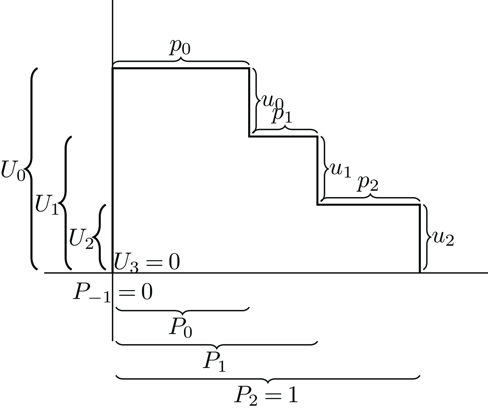


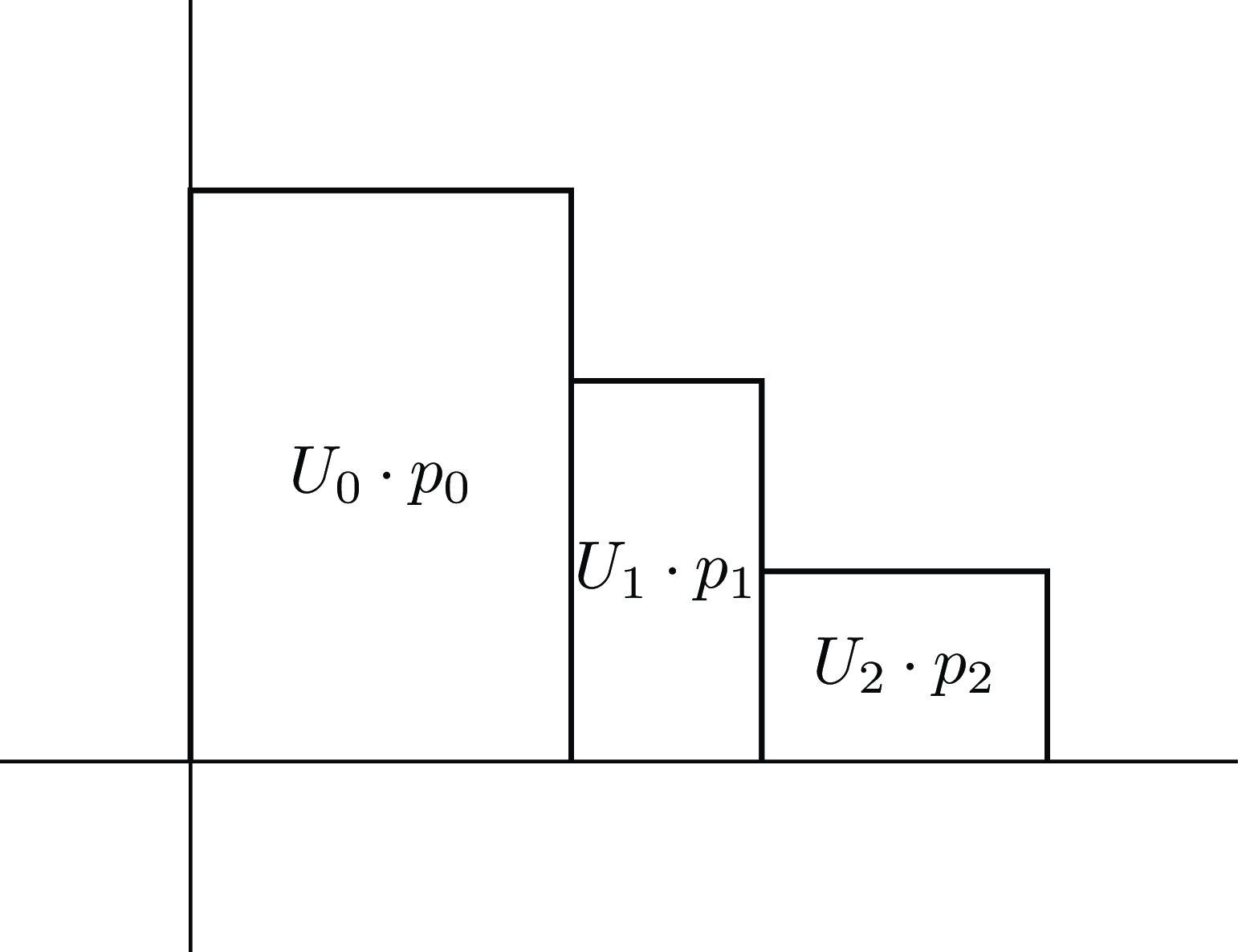
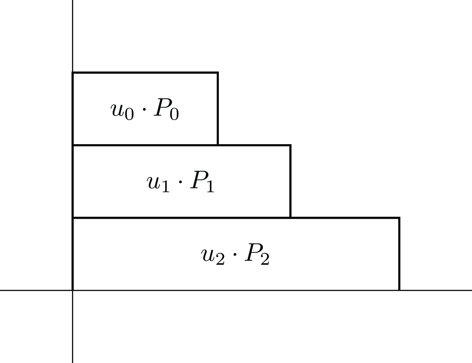
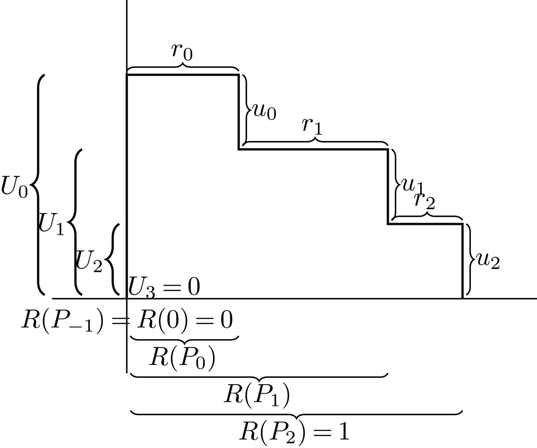


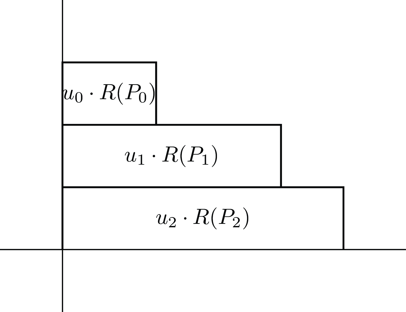
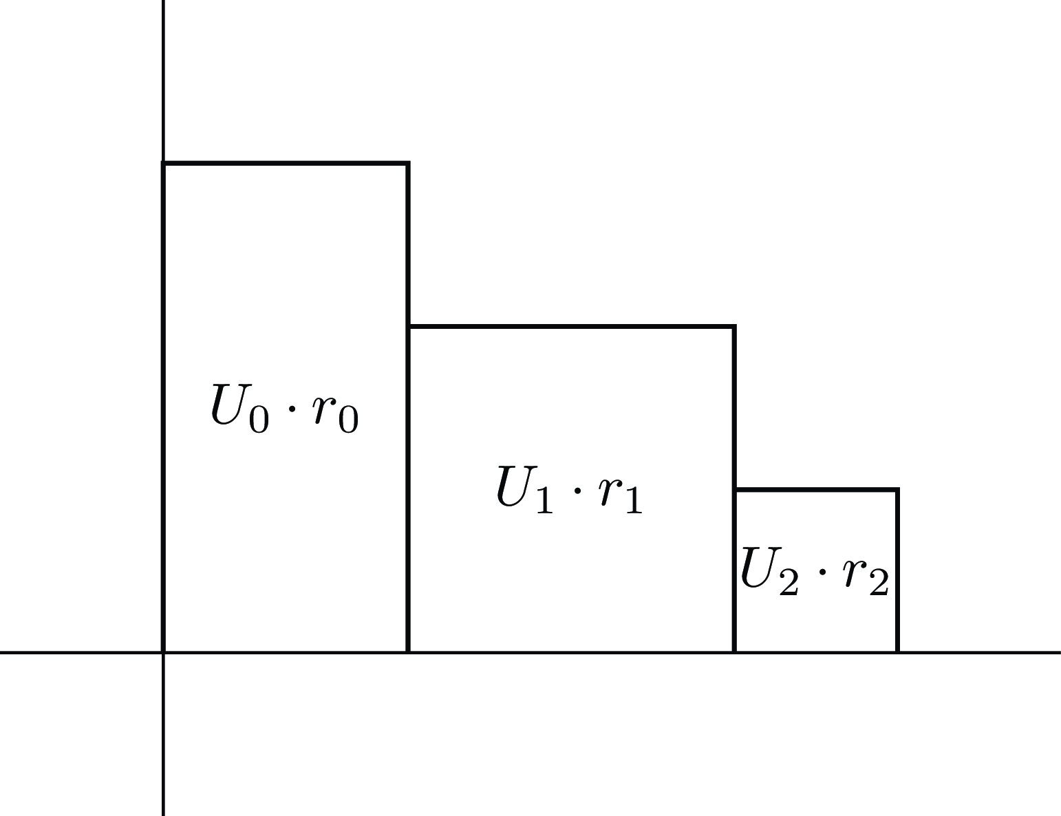
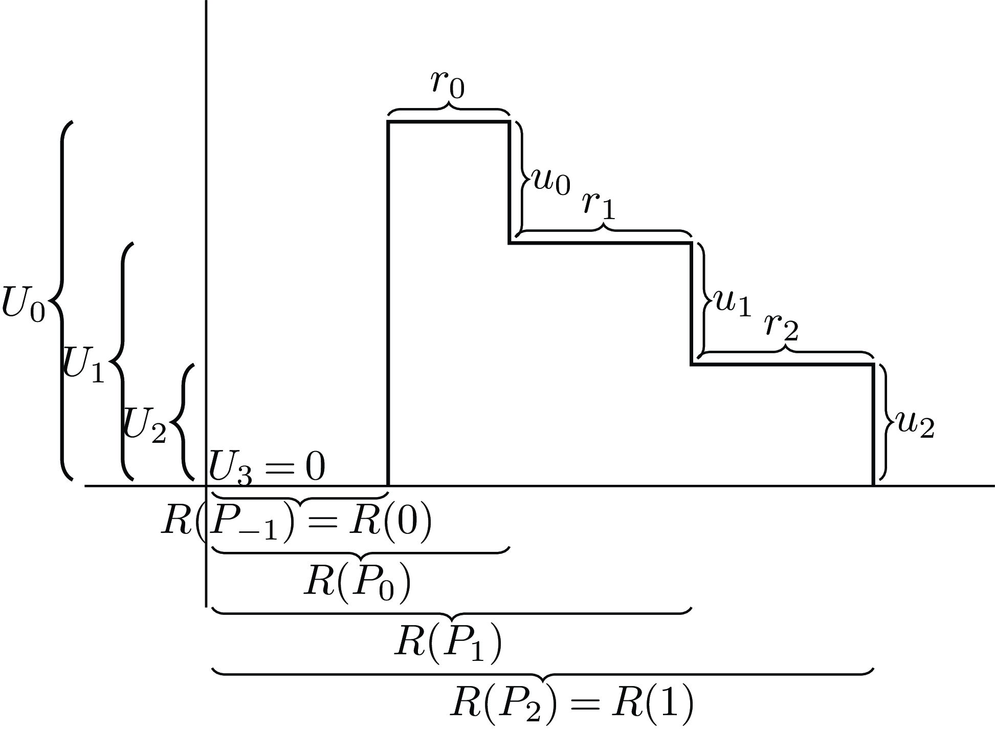

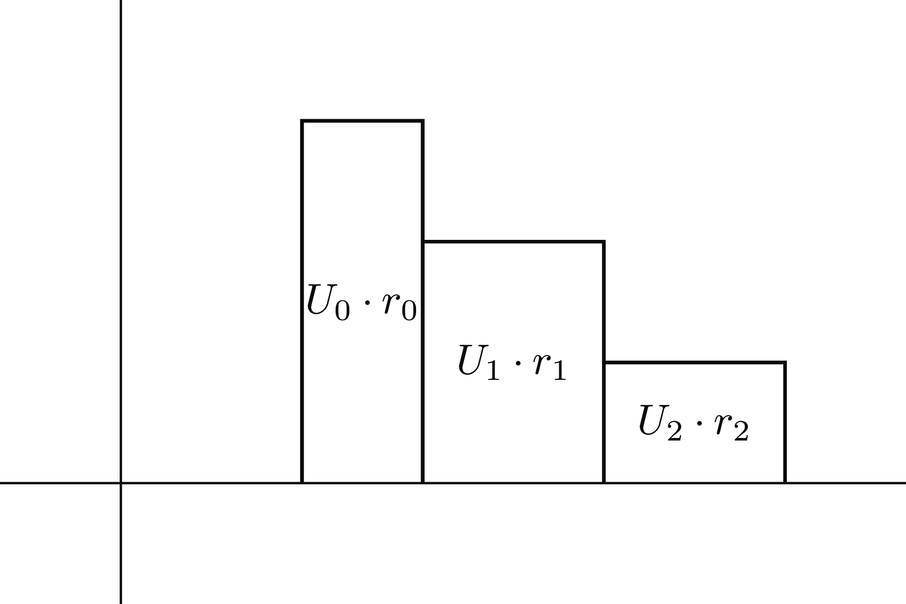

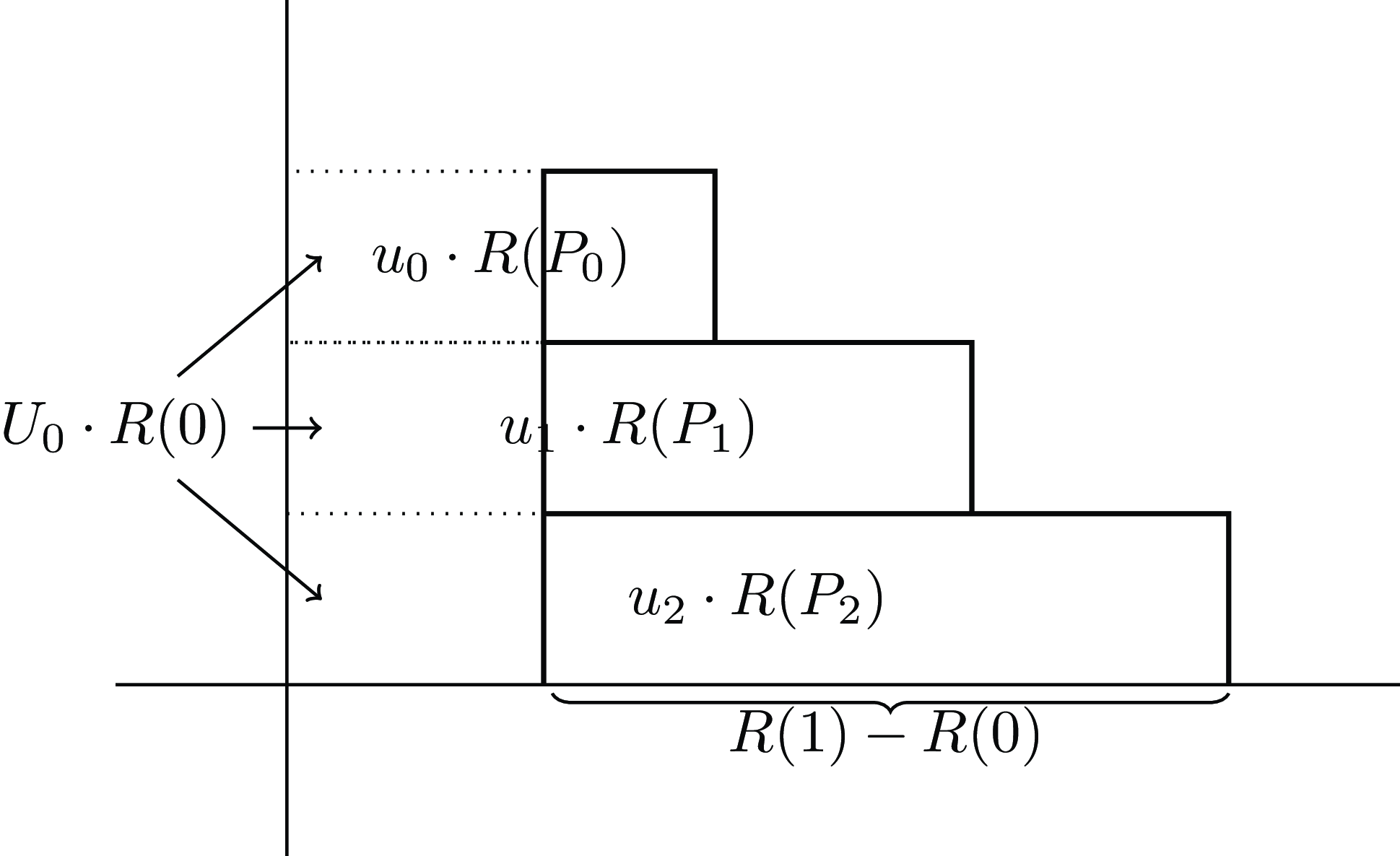

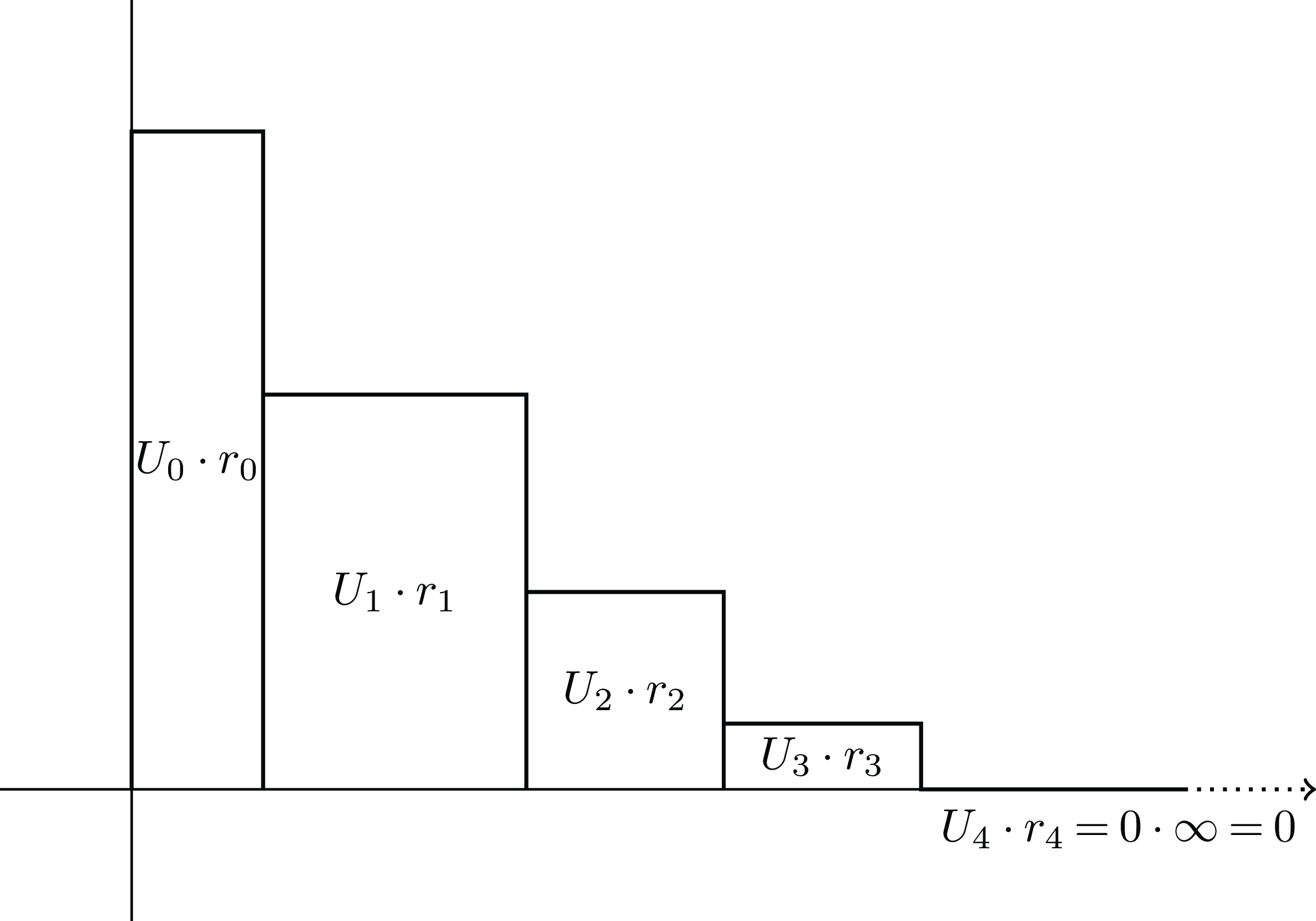


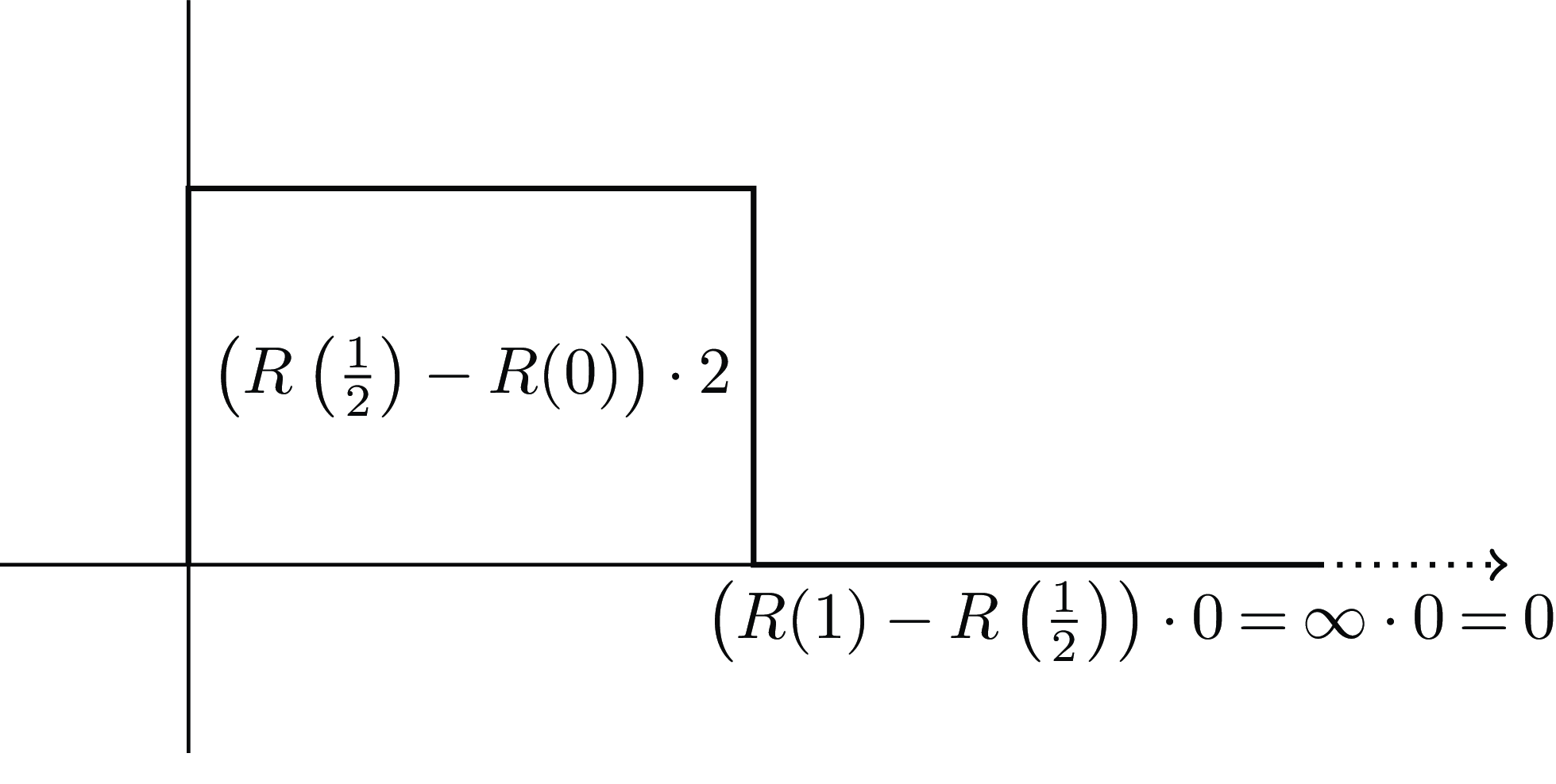


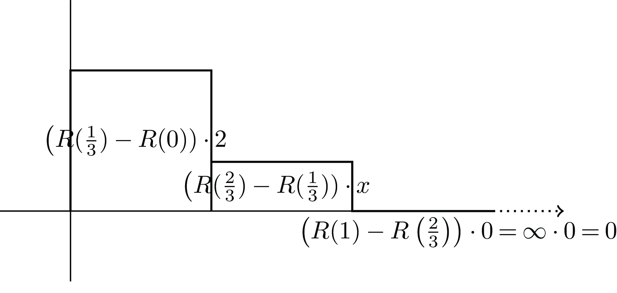


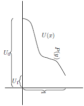


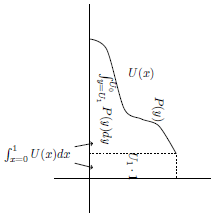


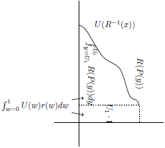
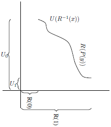


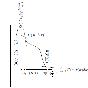


 Open access