


1. Introduction
Since at least the work of Becker, the study of crime and punishment as a problem of economics and choice has received significant attention [Reference Chalfin and McCrary3–Reference Polinsky and Shavell20]. Framed simply, one can conceptualise individuals as rational agents choosing whether or not to commit crimes based on the estimated utility of the two competing choices, while the justice system, by setting standards of proof for conviction and the severity of punishments imposed, attempts to influence this choice in some desired way. Questions then arise as to what the thresholds of evidence or levels of punishments should be that will best optimise some stated objective function; for example, to minimise expected crime rates.
Becker asked how many resources and how much punishment should be used to enforce different kinds of legislation. There, the optimal decisions minimise social loss in income from offences – the sum of damages, costs of apprehension, costs of conviction, and costs of carrying out punishments. This choice of optimal criteria and how it is calculated has led to more discussions. For example, in Becker, the damage to society is the cost of the offence minus the gain to the offender. In other words, the gain for the offender is counted as a gain for society – leading to the conclusion that society should allow efficient crimes. In response, Stigler posits that an offender’s illicit gains should not be counted as society’s gains, suggesting a change to what the legislators should optimise. This view is not without its problems, since society’s decision on what counts as illicit gains changes throughout time [Reference Raskolnikov22]. Others have circumvented the issue by focusing on other optimal conditions or narrowing down the details of the illicit activity being considered. For example, Raskolnikov focused on crime where the illicit gains always equal the harm done. Curry and Doyle introduced a voluntary market option for individuals to achieve the same objective as they would with criminal behaviour. With that, Curry and Doyle showed that minimising the cost of crime corresponds with maximising social welfare. The possibilities to be considered are numerous; Polinsky and Shavell give an excellent overview and discussion on deterrence modelling considerations.
At the same time, a large body of work shows that the justice system often has differential effects on various subgroups of the overall population [Reference Knox, Lowe and Mummolo13–Reference Petersilia17]. Motivated by this, some recent works on the economics of crime have begun to build various metrics of ‘fairness’ into the objective function. A fundamental difficulty with this task is that consensus on a formal definition of fairness is lacking. Further, it is known [Reference Chouldechova4, Reference Kleinberg, Mullainathan and Raghavan11] that some fairness metrics are inherently incompatible with others, such that both cannot possibly be achieved simultaneously. And, since these metrics often test the ‘outcome’ of an algorithm, the issue of fairness is further complicated by the infra-marginality problem, where an outcome test for two groups with different risk distributions can suggest bias in favour of one group even if none exists, or sometimes even if the true bias is in favour of the other group [Reference Simoiu, Corbett-Davies and Goel25]. Which definition of fairness is most desirable transcends mathematics and requires moral arguments and philosophical discussions [Reference Loi and Heitz14, Reference Hu7].
Despite these caveats about fairness, generally, researchers on the economics of crime simply choose a plausible notion of fairness and proceed from there, cognisant that their choice may not be shared by all. For example, Persico proposed a model that imposes a fairness restriction for the police such that police behaviour is defined as fair when they police two subgroups with the same intensity; this is coupled with the goal of maximising the number of successful inspections. Persico concludes that, under certain conditions, forcing the police to behave more fairly reduces the overall crime rate. As an alternative notion, Jung et al. consider fairness as an equality in conditional false positive rates between groups, and also show that the crime rate is minimised when this constraint is upheld. Our work adopts this same notion of fairness and shares many other traits with Jung et al. However, due to some key differences between our model and that of Jung et al., we find that equalising false positive rates between groups generally does not minimise crime, nor optimise a general objective function, if it is indeed even possible in the first place. However, we show that under certain circumstances and objective function choices, the fair scenario is in fact the global optimiser.
This work aims to accomplish the following. First, to introduce a model of crime and deterrence that, while certainly only a vastly simplified version of reality, includes certain notions not otherwise included in prior models of this type. This is done in Section 2, in which we will discuss Jung et al.’s baseline model and introduce our own, highlighting the key differences. Second, based on our model, we aim to explore how the crime rate of society depends on the various choices of the justice system and to determine how the justice system might ‘optimally’ achieve a goal of lowering crime while still keeping in mind the negative impact that punishment can have on innocent individuals. This is done in Section 3, where we will explore how the crime rate of a single group reacts with respect to the threshold $\tau$
set by the judge and the punishment level
$\tau$
set by the judge and the punishment level $\kappa$
set by the legislator, and in which we introduce a single group objective function and find optimal values of
$\kappa$
set by the legislator, and in which we introduce a single group objective function and find optimal values of $\tau$
and
$\tau$
and $\kappa$
under a variety of circumstances. Finally, to determine based on the model whether or not a specific notion of fairness between groups can be accomplished, and what optimality for the justice system might look like when this fairness consideration for two groups is included in the objective function. This is studied in Section 4, where we extend our analysis to the case of two groups and explore how a notion of fairness impacts the objective function previously introduced in Section 3.
$\kappa$
under a variety of circumstances. Finally, to determine based on the model whether or not a specific notion of fairness between groups can be accomplished, and what optimality for the justice system might look like when this fairness consideration for two groups is included in the objective function. This is studied in Section 4, where we extend our analysis to the case of two groups and explore how a notion of fairness impacts the objective function previously introduced in Section 3.
2. Setup and baseline model overview
Footnote
1
We start with a version of Jung et al.’s model. Individuals in a societal group $k$
make a binary decision to commit a crime (
$k$
make a binary decision to commit a crime ( $c$
) or to remain innocent (
$c$
) or to remain innocent ( $i$
). An individual who chooses to commit a crime receives reward
$i$
). An individual who chooses to commit a crime receives reward $\rho$
, while an individual who chooses not to commit a crime receives reward
$\rho$
, while an individual who chooses not to commit a crime receives reward $\nu$
. The difference between these two quantities is
$\nu$
. The difference between these two quantities is $\gamma \equiv \rho - \nu$
, and varies from person to person within the group since opportunities both within and outside of crime might naturally vary; let the density
$\gamma \equiv \rho - \nu$
, and varies from person to person within the group since opportunities both within and outside of crime might naturally vary; let the density $\Gamma _k(\gamma )$
represent the distribution of this quantity within the group. Clearly, those individuals with
$\Gamma _k(\gamma )$
represent the distribution of this quantity within the group. Clearly, those individuals with $\gamma \leq 0$
have no quantitative incentive to commit crime, while those with
$\gamma \leq 0$
have no quantitative incentive to commit crime, while those with $\gamma \gt 0$
do. We will assume throughout that the density
$\gamma \gt 0$
do. We will assume throughout that the density $\Gamma _k \geq 0$
is strictly positive at all positive
$\Gamma _k \geq 0$
is strictly positive at all positive $\gamma$
values, indicating that it contains some mass in the positive
$\gamma$
values, indicating that it contains some mass in the positive $\gamma$
region so that there are at least some individuals who are motivated to commit crime.Footnote
2
$\gamma$
region so that there are at least some individuals who are motivated to commit crime.Footnote
2
Table 1. List of important model parameters and notations with their definition and/or interpretation in plain language ordered by appearance

Each individual within the group may come under suspicion or scrutiny as a possible criminal and be ‘investigated’ or ‘policed’. Let the group-dependent policing rate for those who choose to commit a crime and those who do not be denoted as $\alpha _k$
and
$\alpha _k$
and $\beta _k$
, respectively. We will generally assume that
$\beta _k$
, respectively. We will generally assume that $\alpha _k\geq \beta _k$
, throughout, in the hope that criminals are at least as likely to be investigated as those who are innocent. Each individual who comes under such scrutiny will produce a random ‘signal’
$\alpha _k\geq \beta _k$
, throughout, in the hope that criminals are at least as likely to be investigated as those who are innocent. Each individual who comes under such scrutiny will produce a random ‘signal’ $s\geq 0$
that represents effectively the amount of evidence that appears to indicate guilt for that individual. The distribution of signals for criminals and innocents within group
$s\geq 0$
that represents effectively the amount of evidence that appears to indicate guilt for that individual. The distribution of signals for criminals and innocents within group $k$
is denoted as
$k$
is denoted as $\theta _k^c(s)$
and
$\theta _k^c(s)$
and $\theta _k^i(s)$
, respectively. We assume, as in Jung et al., that these signals exhibit a Monotone Likelihood Ratio Property (MLRP), meaning that
$\theta _k^i(s)$
, respectively. We assume, as in Jung et al., that these signals exhibit a Monotone Likelihood Ratio Property (MLRP), meaning that $\frac {\theta _k^c(s)}{\theta _k^i(s)}$
is nondecreasing in
$\frac {\theta _k^c(s)}{\theta _k^i(s)}$
is nondecreasing in $s.$
That is, a higher signal
$s.$
That is, a higher signal $s$
never denotes a lower likelihood of being guilty vs innocent. For concreteness, throughout the rest of this work, we will assume that the signals
$s$
never denotes a lower likelihood of being guilty vs innocent. For concreteness, throughout the rest of this work, we will assume that the signals $s$
are drawn from exponential distributions
$s$
are drawn from exponential distributions
 \begin{align} \theta _k^i(s) &= \lambda _k e^{-\lambda _k s},\,\lambda _k\gt 0\\[-5pt]\nonumber \end{align}
 \begin{align} \theta _k^c(s) &= \omega _k e^{-\omega _k s},\,\omega _k\gt 0 \end{align}
and we define
 \begin{equation*} p_k\equiv \frac {\omega _k}{\lambda _k}\lt 1 \end{equation*}
to guarantee the MLRP. One can interpret the parameter $p_k$
as essentially indicating how ‘easy’ it is to determine those who are guilty vs innocent within the group
$p_k$
as essentially indicating how ‘easy’ it is to determine those who are guilty vs innocent within the group $k$
, with
$k$
, with $p_k$
close to zero indicating that this determination is relatively easy, and
$p_k$
close to zero indicating that this determination is relatively easy, and $p_k$
near one indicating that the determination is relatively hard.
$p_k$
near one indicating that the determination is relatively hard.
Finally, a judge determines whether the evidence indicates guilt, denoted by $z=1$
, or innocence, denoted by
$z=1$
, or innocence, denoted by $z=0$
, for each individual under scrutiny. In contrast to Jung et al., we focus entirely on the case in which the judge determines guilt versus innocence based on the posterior probability of the individual being a criminal, rather than making the decision based directly on the signal. That is, an individual is classified as guilty if the judge determines that their posterior probability of being a criminal given their signal, their group, and a prior belief on guilt is larger than some threshold
$z=0$
, for each individual under scrutiny. In contrast to Jung et al., we focus entirely on the case in which the judge determines guilt versus innocence based on the posterior probability of the individual being a criminal, rather than making the decision based directly on the signal. That is, an individual is classified as guilty if the judge determines that their posterior probability of being a criminal given their signal, their group, and a prior belief on guilt is larger than some threshold $0\lt \tau \lt 1$
, i.e.
$0\lt \tau \lt 1$
, i.e. $P(c|s,k) \gt \tau$
; otherwise they are found innocent. The details of this assessment will be provided later. Jung et al. instead focus on policies that are based directly on the signal itself, and which are also based on simple thresholding. There is a discussion within Jung et al. of the possibility of posterior thresholding, in which the authors point out that there is rough equivalency between these two methods – a threshold on signal can be translated to a threshold on posterior and vice versa – as we will elaborate on below. However, for the policy problem that is presented in Jung et al., minimising total crime across groups, it is generally true that the optimal policy will correspond to posterior thresholds that are different for different groups. Here is where our approach fundamentally differs: we will insist in this work that only one posterior threshold exists,
$P(c|s,k) \gt \tau$
; otherwise they are found innocent. The details of this assessment will be provided later. Jung et al. instead focus on policies that are based directly on the signal itself, and which are also based on simple thresholding. There is a discussion within Jung et al. of the possibility of posterior thresholding, in which the authors point out that there is rough equivalency between these two methods – a threshold on signal can be translated to a threshold on posterior and vice versa – as we will elaborate on below. However, for the policy problem that is presented in Jung et al., minimising total crime across groups, it is generally true that the optimal policy will correspond to posterior thresholds that are different for different groups. Here is where our approach fundamentally differs: we will insist in this work that only one posterior threshold exists, $\tau$
, and then frame our policy problem under this constraint. We make this choice because one focus of this work is on exploring fairness within the context of this problem, and having separate posterior thresholds for each societal group may violate general ethical and/or legal standards held in many societies; this, despite evidence that in reality these standards are sometimes violated [Reference Knox, Lowe and Mummolo13–Reference Fryer6].
$\tau$
, and then frame our policy problem under this constraint. We make this choice because one focus of this work is on exploring fairness within the context of this problem, and having separate posterior thresholds for each societal group may violate general ethical and/or legal standards held in many societies; this, despite evidence that in reality these standards are sometimes violated [Reference Knox, Lowe and Mummolo13–Reference Fryer6].
As a final aspect of the model, anyone found guilty receives punishment $\kappa$
, set by the legislator, regardless of group. As with the common posterior threshold mentioned above, this assumption comports with general ethical and/or legal standards held in many societies, despite evidence that in reality these standards are sometimes violated [Reference Knox, Lowe and Mummolo13–Reference Fryer6]. In practice, legislators often set a range of punishment levels that judges can choose from to assign to individuals found guilty. But, we will later show that in our framework, the legislator is able to find a single optimal punishment level according to a specific objective function. So, throughout this work, we will assume that the legislator only picks one single punishment level
$\kappa$
, set by the legislator, regardless of group. As with the common posterior threshold mentioned above, this assumption comports with general ethical and/or legal standards held in many societies, despite evidence that in reality these standards are sometimes violated [Reference Knox, Lowe and Mummolo13–Reference Fryer6]. In practice, legislators often set a range of punishment levels that judges can choose from to assign to individuals found guilty. But, we will later show that in our framework, the legislator is able to find a single optimal punishment level according to a specific objective function. So, throughout this work, we will assume that the legislator only picks one single punishment level $\kappa$
for the entire society, which could be the optimal one. This assumption could be relaxed to form a model closer to reality, but with more complications, including a more complex calculation on the part of the society members that would include a probability distribution of
$\kappa$
for the entire society, which could be the optimal one. This assumption could be relaxed to form a model closer to reality, but with more complications, including a more complex calculation on the part of the society members that would include a probability distribution of $\kappa$
values that they might receive; this may be considered in future work.
$\kappa$
values that they might receive; this may be considered in future work.
Given the above, an individual then chooses to commit a crime if their expected net utility from committing a crime is higher than not committing crime. The inequality governing an individual’s decision to commit a crime then becomes
 \begin{align} \rho - \alpha _k \kappa P(z=1|c,k) \gt \nu - \beta _k \kappa P(z=1|i,k). \end{align}
Rearranged, we have
 \begin{align} \kappa \Delta _k & \lt \rho - \nu = \gamma , \end{align}
where
 \begin{align} \Delta _k \equiv \alpha _k P(z=1|c,k) - \beta _k P(z=1|i,k)=TPR_k-FPR_k \end{align}
is a measure of the difference in probability of being found guilty for criminals and innocents within group $k$
, and is therefore the difference between the true positive rate
$k$
, and is therefore the difference between the true positive rate $TPR_k$
and false positive rate
$TPR_k$
and false positive rate $FPR_k$
for group
$FPR_k$
for group $k$
. Then the overall crime rate, measured as the fraction of people choosing to commit crime for group
$k$
. Then the overall crime rate, measured as the fraction of people choosing to commit crime for group $k$
satisfies
$k$
satisfies
 \begin{align} C_k = \int _{\kappa \Delta _k}^{\infty }\Gamma _k(\gamma ) \ d \gamma . \end{align}
We assume that the judge has knowledge of the relevant parameters and distributions for all groups, and can then use this knowledge to aid in determining guilt versus innocence for an individual producing a given signal $s$
. Specifically, the judge makes a Bayesian posterior calculation on the probability of an individual being a criminal based on their signal, group membership, and the known society-wide crime rate
$s$
. Specifically, the judge makes a Bayesian posterior calculation on the probability of an individual being a criminal based on their signal, group membership, and the known society-wide crime rate $C$
, then decides guilt vs innocence based on the threshold value
$C$
, then decides guilt vs innocence based on the threshold value $\tau$
on this posterior probability. Let the society-wide crime rate be computed as
$\tau$
on this posterior probability. Let the society-wide crime rate be computed as
 \begin{equation*} C=\sum _{k=1}^{\mathcal{G}} N_kC_k, \end{equation*}
where $\mathcal{G}$
is the number of distinct societal groups (however these might be defined) and
$\mathcal{G}$
is the number of distinct societal groups (however these might be defined) and $N_k$
and
$N_k$
and $C_k$
are the fraction of the total society that belongs to group
$C_k$
are the fraction of the total society that belongs to group $k$
and the crime rate of group
$k$
and the crime rate of group $k$
, respectively. The posterior probability of an individual being a criminal after observing some signal
$k$
, respectively. The posterior probability of an individual being a criminal after observing some signal $s$
given a group
$s$
given a group $k$
is
$k$
is
 \begin{align} P(c|s,k) = \frac {\alpha _k \theta _k^c(s) C}{\alpha _k \theta _k^c(s) C + \beta _k \theta _k^i(s)(1- C)}. \end{align}
We note that, from the point of view of an accurate posterior probability, equation (2.7) should use $C_k$
rather than
$C_k$
rather than $C$
. However, doing so would essentially represent a prejudice on the part of the judge toward convicting certain groups more readily than others. Since one focus of our work is enforcing fairness within the model, and such a prejudice could readily be construed as unfair, we opt to consider the less biased calculation that uses
$C$
. However, doing so would essentially represent a prejudice on the part of the judge toward convicting certain groups more readily than others. Since one focus of our work is enforcing fairness within the model, and such a prejudice could readily be construed as unfair, we opt to consider the less biased calculation that uses $C$
rather than
$C$
rather than $C_k$
.
$C_k$
.
Recall that an individual is classified as guilty ( $z=1)$
if their posterior probability of being a criminal is greater than the threshold set by the judge,
$z=1)$
if their posterior probability of being a criminal is greater than the threshold set by the judge, $P(c|s,k) \gt \tau$
, with
$P(c|s,k) \gt \tau$
, with $0\lt \tau \lt 1$
. Then, a crime rate of zero would lead to no one ever being found guilty via (2.7). However, in this circumstance, those individuals with
$0\lt \tau \lt 1$
. Then, a crime rate of zero would lead to no one ever being found guilty via (2.7). However, in this circumstance, those individuals with $\gamma \gt 0$
will certainly commit crimes, since they will be guaranteed not to be punished, leading to a contradiction. Hence, it must be the case that
$\gamma \gt 0$
will certainly commit crimes, since they will be guaranteed not to be punished, leading to a contradiction. Hence, it must be the case that $ C_k\gt 0$
, i.e., there will always be some non-zero level of crime if individuals with
$ C_k\gt 0$
, i.e., there will always be some non-zero level of crime if individuals with $\gamma \gt 0$
exist. Because of this and our assumption about the distributions
$\gamma \gt 0$
exist. Because of this and our assumption about the distributions $\theta$
, without loss of generality, we can rewrite (2.7) as
$\theta$
, without loss of generality, we can rewrite (2.7) as
 \begin{equation} P(c|s,k) = \left [1 + \frac {\beta _k \theta _k^i(s)}{\alpha _k \theta _k^c(s)}\frac {(1- C)}{ C}\right ]^{-1}. \end{equation}
Due again to the MLRP for the distributions $\theta _k^i$
and
$\theta _k^i$
and $\theta _k^c$
, for any given crime rate
$\theta _k^c$
, for any given crime rate $ C\lt 1$
the posterior probability of guilt increases with increasing signal, approaching unity as
$ C\lt 1$
the posterior probability of guilt increases with increasing signal, approaching unity as $s\to \infty$
and having a minimum value at
$s\to \infty$
and having a minimum value at $s=0$
; for
$s=0$
; for $ C=1$
the probability is always (correctly) unity for any signal. Then for any
$ C=1$
the probability is always (correctly) unity for any signal. Then for any $ C\lt 1$
and decision threshold
$ C\lt 1$
and decision threshold $\tau$
, there will always exist a threshold signal value
$\tau$
, there will always exist a threshold signal value $s_\tau$
such that only those individuals with
$s_\tau$
such that only those individuals with $s\geq s_\tau$
are found guilty. If
$s\geq s_\tau$
are found guilty. If $\tau \leq P(c|0,k)\equiv \tau _0$
this threshold is just
$\tau \leq P(c|0,k)\equiv \tau _0$
this threshold is just $s_\tau =0$
: everyone is always found guilty in this case. Otherwise, the signal threshold is given by
$s_\tau =0$
: everyone is always found guilty in this case. Otherwise, the signal threshold is given by
 \begin{align} s_\tau = -\frac {1}{\lambda _k - \omega _k} \ln \left (\frac {p_k\alpha _k}{\beta _k}\chi \right )\!, \end{align}
where
 \begin{equation*} \chi \equiv \frac {C}{1-C}\frac {1-\tau }{\tau }. \end{equation*}
To reiterate, whenever
 \begin{align} f_k\equiv \frac {p_k\alpha _k}{\beta _k}\chi =\frac {p_k\alpha _k}{\beta _k}\frac {C}{1-C}\frac {1-\tau }{\tau } \leq 1 \end{align}
then the signal threshold is given by (2.9); otherwise we are in the regime where $\tau \leq \tau _0$
and everyone is found guilty for all signals, so that
$\tau \leq \tau _0$
and everyone is found guilty for all signals, so that $s_\tau =0$
and we can effectively set
$s_\tau =0$
and we can effectively set $f_k=1$
. The existence of a unique
$f_k=1$
. The existence of a unique $s_\tau$
for each
$s_\tau$
for each $\tau$
highlights the equivalency between posterior and signal thresholding mentioned above.
$\tau$
highlights the equivalency between posterior and signal thresholding mentioned above.
We can now compute the total probability of being found guilty conditional on investigation for both criminals and innocents of group $k$
:
$k$
:
 \begin{align} P(z=1|i,k) &= P(s\geq s_\tau |i,k) = \int _{s_\tau }^\infty \theta _k^i(s) \ ds = e^{-\lambda _k s_\tau } = [\min (f_k,1)]^{\frac {1}{1-p_k}}\\[-8pt]\nonumber \end{align}
 \begin{align} P(z=1|c,k) &= P(s\geq s_\tau |c,k) = \int _{s_\tau }^\infty \theta _k^c(s) \ ds = e^{-\omega _k s_\tau } = [\min (f_k,1)]^{\frac {p_k}{1-p_k}}. \end{align}
Multiplying the quantities in (2.11) and (2.12) by $\beta$
and
$\beta$
and $\alpha$
, respectively, gives the false positive rate
$\alpha$
, respectively, gives the false positive rate $FRP_k$
and true positive rate
$FRP_k$
and true positive rate $TPR_k$
for group
$TPR_k$
for group $k$
. Plugging equations (2.11) and (2.12) into equation (2.5), and being careful of inequality (2.10) we have
$k$
. Plugging equations (2.11) and (2.12) into equation (2.5), and being careful of inequality (2.10) we have
 \begin{equation} \Delta _k = \begin{cases} \alpha _k f_k^{\frac {p_k}{1-p_k}} - \beta _k f_k^{\frac {1}{1-p_k}}, & f_k \leq 1\\[5pt] \alpha _k - \beta _k, & f_k \gt 1. \end{cases} \end{equation}
We observe that since $0\lt p_k \lt 1$
,
$0\lt p_k \lt 1$
, $\frac {p_k}{1-p_k} \lt \frac {1}{1-p_k}.$
So,
$\frac {p_k}{1-p_k} \lt \frac {1}{1-p_k}.$
So, $f_k^{\frac {p_k}{1-p_k}} \geq f_k^{\frac {1}{1-p_k}}$
when
$f_k^{\frac {p_k}{1-p_k}} \geq f_k^{\frac {1}{1-p_k}}$
when $f_k\leq 1$
. Combined with our assumption that
$f_k\leq 1$
. Combined with our assumption that $\alpha _k\geq \beta _k$
we have
$\alpha _k\geq \beta _k$
we have $TPR_k\geq FPR_k$
and
$TPR_k\geq FPR_k$
and $\Delta _k\geq 0$
.
$\Delta _k\geq 0$
.
Given all of the group-dependent parameters, as well as $\tau$
and
$\tau$
and $\kappa$
, (2.6) is an implicit equation for the crime rate
$\kappa$
, (2.6) is an implicit equation for the crime rate $C_k$
. In the remainder of this work, we study solutions to this equation in both the single group and two-group cases, and use the crime rates obtained to solve optimisation problems for
$C_k$
. In the remainder of this work, we study solutions to this equation in both the single group and two-group cases, and use the crime rates obtained to solve optimisation problems for $\tau$
and
$\tau$
and $\kappa$
.
$\kappa$
.
3. One group
In this section, we will focus on the properties of solutions to equation (2.6) for one single group. For ease of reading, we drop the subscript $k$
since in this case all parameters and variables belong to a singular group, and in this case,
$k$
since in this case all parameters and variables belong to a singular group, and in this case, $C$
and
$C$
and $C_k$
are identical. We define two functions based on the LHS and RHS of equation (2.6):
$C_k$
are identical. We define two functions based on the LHS and RHS of equation (2.6):
 \begin{align} g(C) & = C \\[-5pt]\nonumber\end{align}
 \begin{align} h(C) & = \int _{\kappa \Delta (C)}^{\infty }\Gamma (\gamma ) \ d \gamma . \end{align}
In (3.2) we have emphasised that $\Delta$
is a function of
$\Delta$
is a function of $C$
. The crime rate solves
$C$
. The crime rate solves $g = h.$
The function
$g = h.$
The function $g$
is straightforward, but we will need to explore the function
$g$
is straightforward, but we will need to explore the function $h$
further. First, we will show that for some parameter region,
$h$
further. First, we will show that for some parameter region, $h$
has a minimum in the interior of its domain as described in the following lemma.
$h$
has a minimum in the interior of its domain as described in the following lemma.
Lemma 3.1. $h(C)$
has a minimum at
$h(C)$
has a minimum at $C_*=\tau$
when
$C_*=\tau$
when $\frac {p \alpha }{\beta } \lt 1.$
The minimum is
$\frac {p \alpha }{\beta } \lt 1.$
The minimum is
 \begin{equation*}h(C_*) = \int _{\kappa \Delta _*}^\infty \Gamma (\gamma ) \ \text{d}\gamma \end{equation*}
where
 \begin{equation*}\Delta _* = \left (\alpha \left (\frac {p\alpha }{\beta }\right )^{\frac {p}{1-p}} - \beta \left (\frac {p\alpha }{\beta }\right )^{\frac {1}{1-p}} \right )\end{equation*}
is a constant.
Proof. Recall that $f$
is a function of
$f$
is a function of $C$
given in (2.10). Then equation (2.13) is equivalent to
$C$
given in (2.10). Then equation (2.13) is equivalent to
 \begin{equation} \Delta = \begin{cases} \alpha f^{\frac {p}{1-p}} - \beta f^{\frac {1}{1-p}}, & C \lt \dfrac {1}{1+ p\frac {\alpha }{\beta }\frac {1-\tau }{\tau }}\\[15pt] \alpha - \beta , & C \geq \dfrac {1}{1+ p\frac {\alpha }{\beta }\frac {1-\tau }{\tau }}, \end{cases} \end{equation}
where $f$
is still a function of
$f$
is still a function of $C$
. And so, when
$C$
. And so, when $C \gt \frac {1}{1+ p\frac {\alpha }{\beta }\frac {1-\tau }{\tau }} \equiv C_0$
,
$C \gt \frac {1}{1+ p\frac {\alpha }{\beta }\frac {1-\tau }{\tau }} \equiv C_0$
,
 \begin{align} h(C)=h(C_0) = \int _{\kappa (\alpha - \beta )}^{\infty }\Gamma (\gamma ) \ \text{d} \gamma , \end{align}
a constant with respect to $C$
. Note that
$C$
. Note that
 \begin{align} h(0) = \int _{0}^{\infty } \Gamma (\gamma ) \ \text{d}\gamma \end{align}
is also a positive constant. The derivative of $h$
is computed to be
$h$
is computed to be
 \begin{align} \frac {\text{d} h}{\text{d} C} &= \begin{cases} -\Gamma (\kappa \Delta ) \kappa \dfrac {\text{d} \Delta }{\text{d} C} =-q(\alpha f^{-1}p - \beta ), & C \lt C_0 \\[8pt] 0, & C \gt C_0. \end{cases} \end{align}
where
 \begin{align} q \equiv \Gamma (\kappa \Delta )\kappa \frac {1}{1-p}\frac {1}{C(1-C)}f^{\frac {1}{1-p}} \gt 0. \end{align}
Then, any critical point $C_*$
of
$C_*$
of $h(C)$
in
$h(C)$
in $(0,C_0)$
can only occur when
$(0,C_0)$
can only occur when $\alpha f^{-1}p - \beta = 0.$
Substituting
$\alpha f^{-1}p - \beta = 0.$
Substituting $f$
from (2.10) and solving, we find the critical point
$f$
from (2.10) and solving, we find the critical point $C_*=\tau$
, which is also equivalent to
$C_*=\tau$
, which is also equivalent to $\chi =1$
. However, this critical point will exist iff
$\chi =1$
. However, this critical point will exist iff $C_* \lt C_0$
; after some algebra this is equivalent to
$C_* \lt C_0$
; after some algebra this is equivalent to
 \begin{align} \frac {p \alpha }{\beta } \lt 1. \end{align}
Under this condition, we have that for $C\lt C_*$
,
$C\lt C_*$
, $\frac {dh}{dC}\lt 0$
, while for
$\frac {dh}{dC}\lt 0$
, while for $C_*\lt C\lt C_0$
we have
$C_*\lt C\lt C_0$
we have $\frac {\text{d}h}{\text{d}C}\gt 0$
, indicating a minimum at
$\frac {\text{d}h}{\text{d}C}\gt 0$
, indicating a minimum at $C=C_*$
. Further,
$C=C_*$
. Further,
 \begin{align} h(C_*) = \int _{\kappa \Delta _*}^\infty \Gamma (\gamma ) \ \text{d}\gamma \end{align}
where
 \begin{align} \Delta _* = \left (\alpha \left (\frac {p\alpha }{\beta }\right )^{\frac {p}{1-p}} - \beta \left (\frac {p\alpha }{\beta }\right )^{\frac {1}{1-p}} \right ) \end{align}
is a constant.
The proof above also leads to the following lemma:
Lemma 3.2. $h(C)$
is monotonically decreasing on
$h(C)$
is monotonically decreasing on $(0,C_0)$
when
$(0,C_0)$
when $\frac {p\alpha }{\beta } \geq 1.$
Next, we will prove a lemma that will help us understand how many times $g$
and
$g$
and $h$
intersect which corresponds to the number of solutions to the crime rate equation.
$h$
intersect which corresponds to the number of solutions to the crime rate equation.
Lemma 3.3. $ \frac {\text{d}h}{\text{d}C} \lt 1$
when
$ \frac {\text{d}h}{\text{d}C} \lt 1$
when $1 - \frac {1}{q \beta } \leq \frac {p \alpha }{\beta }$
for
$1 - \frac {1}{q \beta } \leq \frac {p \alpha }{\beta }$
for $C \in (0,C_0)$
.
$C \in (0,C_0)$
.
Proof. For ease of reading we define $\phi (C) = \alpha f^{-1} p - \beta =\beta \frac {1-C}{C}\frac {\tau }{1-\tau }-\beta .$
We first compute
$\phi (C) = \alpha f^{-1} p - \beta =\beta \frac {1-C}{C}\frac {\tau }{1-\tau }-\beta .$
We first compute
 \begin{align} \frac {\text{d}\phi }{\text{d}C} &= \frac {\text{d}}{\text{d}C}\left(\beta \frac {1-C}{C}\frac {\tau }{1-\tau }\right)\\[-10pt]\nonumber \end{align}
 \begin{align} &= -\beta \frac {1}{C^2}\frac {\tau }{1-\tau } \lt 0. \end{align}
So, in the domain $C \in (0,C_0)$
,
$C \in (0,C_0)$
,
 \begin{align} \phi (C_0)\lt \phi (C) \end{align}
Here, $\phi (C_0) = p \alpha - \beta .$
So, by rearranging our initial assumption and since
$\phi (C_0) = p \alpha - \beta .$
So, by rearranging our initial assumption and since $f^{-1} \gt 1,$
 \begin{align} -\frac {1}{q} \leq p\alpha - \beta \lt \alpha f^{-1} p - \beta . \end{align}
Rearranging, we have
 \begin{align} \frac {\text{d}h}{\text{d}C} = -q(\alpha f^{-1} p - \beta ) \lt 1. \end{align}
The lemmas above lead to the following uniqueness theorem.
Theorem 3.4.
If $1 - \frac {1}{q \beta } \leq \frac {p \alpha }{\beta }$
for
$1 - \frac {1}{q \beta } \leq \frac {p \alpha }{\beta }$
for $C \in (0,C_0)$
then there is a unique solution to equation (2.6
).
$C \in (0,C_0)$
then there is a unique solution to equation (2.6
).
Proof. Recall from equation (3.5) that $0\lt h(0)\leq 1$
. Also,
$0\lt h(0)\leq 1$
. Also, $h(1) \lt h(0)\leq 1$
from properties of cumulative distribution functions and our assumption that
$h(1) \lt h(0)\leq 1$
from properties of cumulative distribution functions and our assumption that $\Gamma \gt 0$
. We have
$\Gamma \gt 0$
. We have $g(0) = 0$
and
$g(0) = 0$
and $ g(1) = 1$
. If
$ g(1) = 1$
. If $\frac {p \alpha }{\beta } \geq 1,$
then
$\frac {p \alpha }{\beta } \geq 1,$
then $h(c)$
is monotonic by Lemma 3.2. And so there must only be one intersection between
$h(c)$
is monotonic by Lemma 3.2. And so there must only be one intersection between $g(C)$
and
$g(C)$
and $h(C).$
If
$h(C).$
If $1-\frac {1}{q \beta } \leq \frac {p \alpha }{\beta } \lt 1$
for
$1-\frac {1}{q \beta } \leq \frac {p \alpha }{\beta } \lt 1$
for $C \in (0,C_0)$
, then by Lemma 3.3,
$C \in (0,C_0)$
, then by Lemma 3.3, $\frac {dh}{dC} \lt 1 = \frac {dg}{dC}.$
Similarly, there must be only one intersection between
$\frac {dh}{dC} \lt 1 = \frac {dg}{dC}.$
Similarly, there must be only one intersection between $g(C)$
and
$g(C)$
and $h(C).$
However, if it is the case that $\frac {p \alpha }{\beta }\lt 1-\frac {1}{q\beta }$
for some
$\frac {p \alpha }{\beta }\lt 1-\frac {1}{q\beta }$
for some $C \in (0,C_0)$
, there could be multiple solutions, as illustrated in Figure 1. To summarise the findings of the theorems above and as illustrated in Figure 1, when
$C \in (0,C_0)$
, there could be multiple solutions, as illustrated in Figure 1. To summarise the findings of the theorems above and as illustrated in Figure 1, when $ \frac {p \alpha }{\beta } \geq 1$
there is a unique crime rate for any given
$ \frac {p \alpha }{\beta } \geq 1$
there is a unique crime rate for any given $\tau$
and
$\tau$
and $\kappa$
, and the crime rate is increasing with
$\kappa$
, and the crime rate is increasing with $\tau$
for any
$\tau$
for any $\tau \gt \tau _0$
; that is, crime is minimised when everyone investigated is found guilty. On the other hand, when
$\tau \gt \tau _0$
; that is, crime is minimised when everyone investigated is found guilty. On the other hand, when $ \frac {p \alpha }{\beta } \lt 1$
, there are potentially multiple crime rates consistent with (2.6) for certain
$ \frac {p \alpha }{\beta } \lt 1$
, there are potentially multiple crime rates consistent with (2.6) for certain $\tau$
and
$\tau$
and $\kappa$
. However, there is a threshold
$\kappa$
. However, there is a threshold $\tau _*=C_*=h(C_*)$
that yields the smallest crime rate possible, in which not everyone investigated is found guilty.
$\tau _*=C_*=h(C_*)$
that yields the smallest crime rate possible, in which not everyone investigated is found guilty.
Recall that $p= \frac {\omega }{\lambda }\lt 1$
is the ratio of the decay rate of the signal for innocents and the decay rate of the signal for criminals, and that
$p= \frac {\omega }{\lambda }\lt 1$
is the ratio of the decay rate of the signal for innocents and the decay rate of the signal for criminals, and that $p$
closer to 1 indicates that the signal of the criminals and innocents are less distinguishable while lower
$p$
closer to 1 indicates that the signal of the criminals and innocents are less distinguishable while lower $p$
indicates that the signal of criminals and innocents are more distinguishable. Similarly, the ratio
$p$
indicates that the signal of criminals and innocents are more distinguishable. Similarly, the ratio $\frac {\beta }{\alpha }$
denotes how different the policing rate is for innocents vs. criminals, with a low ratio meaning that innocents are policed notably less than criminals and a ratio approaching 1 indicating that they are policed at essentially the same rate. Let us rewrite the region
$\frac {\beta }{\alpha }$
denotes how different the policing rate is for innocents vs. criminals, with a low ratio meaning that innocents are policed notably less than criminals and a ratio approaching 1 indicating that they are policed at essentially the same rate. Let us rewrite the region $\frac {p \alpha }{\beta } \lt 1$
instead as
$\frac {p \alpha }{\beta } \lt 1$
instead as $p \lt \frac {\beta }{\alpha }.$
Then this region corresponds to one in which the signals between the innocents and the criminals are more distinguishable than their policing rate ratio would suggest. Intuitively, this means that the judge is able to add something valuable to the guilt determination process, and further narrow down who is guilty vs innocent beyond the relatively crude distinction made by the police. Because of this, the judge can choose a threshold
$p \lt \frac {\beta }{\alpha }.$
Then this region corresponds to one in which the signals between the innocents and the criminals are more distinguishable than their policing rate ratio would suggest. Intuitively, this means that the judge is able to add something valuable to the guilt determination process, and further narrow down who is guilty vs innocent beyond the relatively crude distinction made by the police. Because of this, the judge can choose a threshold $\tau _*$
that minimises crime rate without finding everyone guilty, as shown above. Conversely, the region
$\tau _*$
that minimises crime rate without finding everyone guilty, as shown above. Conversely, the region $\frac {p \alpha }{\beta } \geq 1$
, equivalently
$\frac {p \alpha }{\beta } \geq 1$
, equivalently $p \geq \frac {\beta }{\alpha },$
corresponds to the case where the signals between the innocents and criminals are at most as distinguishable as their policing rate ratio would suggest. In other words, the judge is not as efficient as the police in determining guilt vs innocence, and does not add much of value to the process. Here, the judge minimises crime by just finding everyone guilty, as in this case, the police will have already largely been able to determine guilt before any trial occurs. Generally, it seems plausible that the former case, where the judge is better able to determine guilt vs innocence than the police, is the more realistic of the two.
$p \geq \frac {\beta }{\alpha },$
corresponds to the case where the signals between the innocents and criminals are at most as distinguishable as their policing rate ratio would suggest. In other words, the judge is not as efficient as the police in determining guilt vs innocence, and does not add much of value to the process. Here, the judge minimises crime by just finding everyone guilty, as in this case, the police will have already largely been able to determine guilt before any trial occurs. Generally, it seems plausible that the former case, where the judge is better able to determine guilt vs innocence than the police, is the more realistic of the two.
In the next two subsections, we will discuss the case where there could be multiple solutions. Then, we will explore how the crime rate changes in relation to the threshold $\tau$
and the punishment level
$\tau$
and the punishment level $\kappa$
and consider a reasonable objective function for the judge and the legislator to minimise.
$\kappa$
and consider a reasonable objective function for the judge and the legislator to minimise.

Figure 1. Intersection(s) of $g(C)$
and
$g(C)$
and $h(C)$
. The dashed lines from top to bottom correspond to the regions
$h(C)$
. The dashed lines from top to bottom correspond to the regions $\frac {p \alpha }{\beta } \geq 1$
,
$\frac {p \alpha }{\beta } \geq 1$
, $1 -\frac {1}{qb} \lt \frac {p \alpha }{\beta } \lt 1$
, and
$1 -\frac {1}{qb} \lt \frac {p \alpha }{\beta } \lt 1$
, and $\frac {p \alpha }{\beta } \lt 1 -\frac {1}{qb}$
, respectively. The solid horizontal line indicates the region in which
$\frac {p \alpha }{\beta } \lt 1 -\frac {1}{qb}$
, respectively. The solid horizontal line indicates the region in which $f=1$
. Panel (a) is constructed at a lower threshold
$f=1$
. Panel (a) is constructed at a lower threshold $\tau$
than that used in (b).
$\tau$
than that used in (b).
3.1. Remark on multiple crime rates
As described above, equation (2.6) may be consistent for several different crime rates $C$
, that is, the solution might not be unique in some parameter regions. In that case, it is not immediately clear which of these consistent crime rates would manifest, as the overall model assumes that criminals can determine their expected utilities perfectly, and those depend on the crime rate observed. However, we will show that, by our assumption that individuals want to maximise their utility, the smallest of these consistent crime rates will be the one to occur.
$C$
, that is, the solution might not be unique in some parameter regions. In that case, it is not immediately clear which of these consistent crime rates would manifest, as the overall model assumes that criminals can determine their expected utilities perfectly, and those depend on the crime rate observed. However, we will show that, by our assumption that individuals want to maximise their utility, the smallest of these consistent crime rates will be the one to occur.
Suppose there are multiple solutions to (2.6), labelled $C^{(1)}\lt C^{(2)}\lt \cdots \lt C^{(n)}$
. Each such crime rate can be thought of as representing a Nash Equilibrium of the system. That is, any solution
$C^{(1)}\lt C^{(2)}\lt \cdots \lt C^{(n)}$
. Each such crime rate can be thought of as representing a Nash Equilibrium of the system. That is, any solution $C^{(i)}$
corresponds to a value
$C^{(i)}$
corresponds to a value $\gamma ^{(i)}$
that has two properties:
$\gamma ^{(i)}$
that has two properties: $C^{(i)}=\int _{\gamma ^{(i)}}^\infty \Gamma (\gamma ) \text{d}\gamma$
(the solution is consistent); and if individuals with
$C^{(i)}=\int _{\gamma ^{(i)}}^\infty \Gamma (\gamma ) \text{d}\gamma$
(the solution is consistent); and if individuals with $\gamma \gt \gamma ^{(i)}$
commit crimes and those with
$\gamma \gt \gamma ^{(i)}$
commit crimes and those with $\gamma \lt \gamma ^{(i)}$
do not, no individual is tempted to deviate from this unilaterally (a Nash Equilibrium). Note that these threshold
$\gamma \lt \gamma ^{(i)}$
do not, no individual is tempted to deviate from this unilaterally (a Nash Equilibrium). Note that these threshold $\gamma$
values lie in the order
$\gamma$
values lie in the order $\gamma ^{(n)}\lt \gamma ^{(n-1)}$ $\lt \cdots \lt \gamma ^{(1)}$
.
$\lt \cdots \lt \gamma ^{(1)}$
.
However, the expected utilities for individuals among these Nash Equilibria are not equal. Note that those with $\gamma \gt \gamma ^{(1)}$
will commit crimes no matter which equilibrium is selected, and those with
$\gamma \gt \gamma ^{(1)}$
will commit crimes no matter which equilibrium is selected, and those with $\gamma \lt \gamma ^{(n)}$
will not commit crimes no matter which is selected, so that we need only consider those individuals with
$\gamma \lt \gamma ^{(n)}$
will not commit crimes no matter which is selected, so that we need only consider those individuals with $\gamma ^{(n)}\lt \gamma \lt \gamma ^{(1)}$
and determine which equilibrium they might prefer. For a fixed behaviour – commit crimes vs not – utility is decreasing with increasing probability of punishment, which itself increases with crime rate. Hence, for any given individual under consideration we need only contrast two of the equilibria:
$\gamma ^{(n)}\lt \gamma \lt \gamma ^{(1)}$
and determine which equilibrium they might prefer. For a fixed behaviour – commit crimes vs not – utility is decreasing with increasing probability of punishment, which itself increases with crime rate. Hence, for any given individual under consideration we need only contrast two of the equilibria: $C^{(1)}$
, in which case they do not commit crime and crime is as low as possible; and
$C^{(1)}$
, in which case they do not commit crime and crime is as low as possible; and $C^{(j)}$
, which is the lowest crime rate for which the corresponding
$C^{(j)}$
, which is the lowest crime rate for which the corresponding $\gamma ^{(j)}$
is less than the
$\gamma ^{(j)}$
is less than the $\gamma$
value of the individual in question, which is the lowest crime state in which that person commits crime. Then this individual will prefer the equilibrium at
$\gamma$
value of the individual in question, which is the lowest crime state in which that person commits crime. Then this individual will prefer the equilibrium at $C^{(1)}$
so long as
$C^{(1)}$
so long as
 \begin{equation*} \nu -\beta \kappa P\left (z=1|i;\,C^{(i)}\right )\gt \rho -\alpha \kappa P\left (z=1|c;\,C^{(j)}\right ). \end{equation*}
Upon rearranging terms and writing existing quantities in terms of $\gamma _1$
, the above inequality is equivalent to
$\gamma _1$
, the above inequality is equivalent to
 \begin{equation*} \gamma \lt \gamma ^{(1)} + \alpha \kappa \left [P\left (z=1|c;\,C^{(j)}\right )-P\left (z=1|c;\,C^{(1)}\right )\right ]. \end{equation*}
Noting that the term in brackets is positive, this inequality holds for all individuals in question, meaning that they all prefer the lowest crime equilibrium above all others. Therefore, even in cases where there are multiple solutions to (2.6), one would expect that the lowest crime solution should be the one obtained.
3.2. Judge’s and legislator’s objective
We now model the choice of $\tau$
and
$\tau$
and $\kappa$
as optimisation problems for the judge and legislator. As a very simple first possibility, perhaps the judge and legislator are working in unison to simply minimise the crime rate
$\kappa$
as optimisation problems for the judge and legislator. As a very simple first possibility, perhaps the judge and legislator are working in unison to simply minimise the crime rate $C$
. Given the results above, for a fixed punishment level
$C$
. Given the results above, for a fixed punishment level $\kappa$
, crime is minimised in one of two ways. First, if
$\kappa$
, crime is minimised in one of two ways. First, if $\frac {p\alpha }{\beta } \geq 1$
, then crime is minimised at rate
$\frac {p\alpha }{\beta } \geq 1$
, then crime is minimised at rate $C_0=h(C_0)$
from (3.4), since
$C_0=h(C_0)$
from (3.4), since $h(C)$
is monotonically decreasing on
$h(C)$
is monotonically decreasing on $(0,C_0)$
in this case. This corresponds to selecting any threshold
$(0,C_0)$
in this case. This corresponds to selecting any threshold $\tau \in (0,\tau _0]$
, in which case all individuals are found guilty, and
$\tau \in (0,\tau _0]$
, in which case all individuals are found guilty, and $\tau _0=1/\left [1+\frac {\beta }{p\alpha }\frac {1-C_0}{C_0}\right ].$
If
$\tau _0=1/\left [1+\frac {\beta }{p\alpha }\frac {1-C_0}{C_0}\right ].$
If $\frac {p\alpha }{\beta } \lt 1$
, then crime is minimised at rate
$\frac {p\alpha }{\beta } \lt 1$
, then crime is minimised at rate $C_*=h(C_*)$
from (3.9), since that is where
$C_*=h(C_*)$
from (3.9), since that is where $h(C)$
is minimised in this case (and cases of multiple solutions here will still exhibit the smallest crime rate possible). This corresponds to selecting threshold
$h(C)$
is minimised in this case (and cases of multiple solutions here will still exhibit the smallest crime rate possible). This corresponds to selecting threshold $\tau =\tau _*=C_*$
; in this case, not all individuals are found guilty. In either of these cases, the crime rate simply decreases with
$\tau =\tau _*=C_*$
; in this case, not all individuals are found guilty. In either of these cases, the crime rate simply decreases with $\kappa$
, indicating that arbitrarily large punishment should be sought, and no global minimum of crime truly exists.
$\kappa$
, indicating that arbitrarily large punishment should be sought, and no global minimum of crime truly exists.
Of course, it is not clear that in reality severe punishment (for a given threshold) always leads to lower crime. This model makes many simplifying assumptions that are perhaps only approximately true, not least of which the idea that the choice to commit crimes is always based on a logical cost–benefit analysis; crimes of passion do exist, after all. This assumption could be relaxed to allow for individuals to commit crimes even if it is not economically beneficial, but we leave that for future work. But beyond this, even if the model were a perfect simulacrum of the criminal justice system, the objective of simply minimising crime does not appear very satisfying. It suggests draconian punishment, ignoring the fact that these punishments are sometimes, unfortunately, meted out to innocent people. Further, it indicates that the posterior threshold for punishment should be very small – either small enough so that all are guilty, or set to match $C_*$
, which is being made as small as possible – which generally conflicts with Western ideals that posteriors at least be “the preponderance of evidence,” if not higher.
$C_*$
, which is being made as small as possible – which generally conflicts with Western ideals that posteriors at least be “the preponderance of evidence,” if not higher.
We therefore propose an alternative objective function. Certainly, low crime is still desired, as that minimises the impact of crime on victims, among many other things. However, this desire should be balanced against harm that could also be done to innocent individuals through erroneous punishment. The portion of the objective indicating harm could take many forms and include many items, such as opportunity costs incurred by punishing innocent individuals, or fear and distrust that very severe punishments might instil in citizens. However, to avoid introducing too many other considerations to the model, we stick with a relatively basic term that can be included without much difficulty, and which essentially directly measures the amount of punishment applied to innocent people. We therefore propose that the judge and legislator might consider the objective function
 \begin{align} M = C +\lambda \kappa ^n(1-C) FPR. \end{align}
Here, $\lambda \gt 0$
and
$\lambda \gt 0$
and $n\gt 0$
are both parameters that change the balance between desiring low crime vs low punishment for innocent individuals who are found guilty. We note that for
$n\gt 0$
are both parameters that change the balance between desiring low crime vs low punishment for innocent individuals who are found guilty. We note that for $n=1$
, a seemingly natural choice, the second term is directly proportional to the total amount of punishment meted out to innocents, with a constant of proportionality
$n=1$
, a seemingly natural choice, the second term is directly proportional to the total amount of punishment meted out to innocents, with a constant of proportionality $\lambda$
. However, as we will show below, choosing
$\lambda$
. However, as we will show below, choosing $n=1$
leads to an unsatisfying solution to the optimisation problem.
$n=1$
leads to an unsatisfying solution to the optimisation problem.
While the natural choice of parameters over which to optimise $M$
are
$M$
are $\kappa$
and
$\kappa$
and $\tau$
, it is easier to analyse the system by choosing to parameterise with
$\tau$
, it is easier to analyse the system by choosing to parameterise with $\kappa$
and
$\kappa$
and $\chi$
. This parametrisation is equivalent, so long as we note that some
$\chi$
. This parametrisation is equivalent, so long as we note that some $\kappa$
,
$\kappa$
, $\chi$
combinations may not be feasible. Specifically, any
$\chi$
combinations may not be feasible. Specifically, any $\kappa$
,
$\kappa$
, $\chi$
combination has a well-defined crime rate, and that crime rate, when combined with
$\chi$
combination has a well-defined crime rate, and that crime rate, when combined with $\chi$
gives a well-defined
$\chi$
gives a well-defined $\tau$
. However, for a given
$\tau$
. However, for a given $\kappa$
, there could exist two (or more) values
$\kappa$
, there could exist two (or more) values $\chi _1\lt \chi _2$
, with corresponding
$\chi _1\lt \chi _2$
, with corresponding $C_1\lt C_2$
that both give the same
$C_1\lt C_2$
that both give the same $\tau$
. As noted above, in such cases when a single
$\tau$
. As noted above, in such cases when a single $\tau$
gives rise to multiple crime rates, only the lowest rate is realisable, hence the combination
$\tau$
gives rise to multiple crime rates, only the lowest rate is realisable, hence the combination $\kappa$
,
$\kappa$
, $\chi _2$
is not feasible. While this could potentially be a problem moving forward, we note that this issue will not arise when
$\chi _2$
is not feasible. While this could potentially be a problem moving forward, we note that this issue will not arise when $\frac {p \alpha }{\beta } \geq 1$
, and even when
$\frac {p \alpha }{\beta } \geq 1$
, and even when $\frac {p \alpha }{\beta }\lt 1$
, we can be sure that any
$\frac {p \alpha }{\beta }\lt 1$
, we can be sure that any $\kappa$
with
$\kappa$
with $\chi \leq 1$
is feasible. This is because, when a single
$\chi \leq 1$
is feasible. This is because, when a single $\tau$
could yield multiple crime rates via (2.6), either one of those crime rates has
$\tau$
could yield multiple crime rates via (2.6), either one of those crime rates has $\chi \leq 1$
and the others have
$\chi \leq 1$
and the others have $\chi \gt 1$
, and the
$\chi \gt 1$
, and the $\chi \leq 1$
rate is the feasible one, or all of the crime rates have
$\chi \leq 1$
rate is the feasible one, or all of the crime rates have $\chi \gt 1$
. We will revisit this point later.
$\chi \gt 1$
. We will revisit this point later.
Seeking critical points of $M$
gives the following equations
$M$
gives the following equations
 \begin{align} \frac {\partial M}{\partial \kappa } &= -\Gamma (\kappa \Delta )\Delta (1-\lambda \kappa ^nFPR) +\lambda n\kappa ^{n-1}(1-C)FPR=0\\[-5pt]\nonumber \end{align}
 \begin{align} \frac {\partial M}{\partial \chi } &=\left [ -\Gamma (\kappa \Delta )\kappa \frac {\partial \Delta }{\partial FPR}(1-\lambda \kappa ^nFPR)+ \lambda \kappa ^{n}(1-C)\right ] \frac {\partial FPR}{\partial \chi }=0 . \end{align}
After some algebra, one can show that in order for there to exist a simultaneous solution to the equations above, it must be the case that
 \begin{align} \chi = \frac {n - \frac {1}{p}}{n-1}\equiv \chi _o. \end{align}
Note that since $\chi \gt 0,$
equation (3.19) requires either that
$\chi \gt 0,$
equation (3.19) requires either that $n\lt 1$
or that
$n\lt 1$
or that $n \gt \frac {1}{p}\gt 1$
in order for such a critical point to exist. The
$n \gt \frac {1}{p}\gt 1$
in order for such a critical point to exist. The $n\lt 1$
case always leads to
$n\lt 1$
case always leads to $f\gt 1$
and therefore should not be considered further. Assuming
$f\gt 1$
and therefore should not be considered further. Assuming $n\gt \frac {1}{p}$
, then
$n\gt \frac {1}{p}$
, then $\chi _o\lt 1$
, which means this is certainly a feasible point. However, we must still determine if
$\chi _o\lt 1$
, which means this is certainly a feasible point. However, we must still determine if $f=\frac {p \alpha }{\beta } \chi _o\leq 1$
. This is automatically the case when
$f=\frac {p \alpha }{\beta } \chi _o\leq 1$
. This is automatically the case when $\frac {p \alpha }{\beta } \lt 1$
; that is, when crime has a minimum at
$\frac {p \alpha }{\beta } \lt 1$
; that is, when crime has a minimum at $C_*$
. However, if
$C_*$
. However, if $\frac {p \alpha }{\beta } \geq 1$
, then this requirement places an upper bound on
$\frac {p \alpha }{\beta } \geq 1$
, then this requirement places an upper bound on $n$
for the existence of the critical point, such that
$n$
for the existence of the critical point, such that $n\lt \frac {\alpha -\beta }{\alpha p - \beta }$
.
$n\lt \frac {\alpha -\beta }{\alpha p - \beta }$
.
Assume for now that all requirements are met for a physically relevant $\chi _o$
. Let
$\chi _o$
. Let $FRP_o$
and
$FRP_o$
and $TPR_o$
be the false positive and true positive rates obtained when
$TPR_o$
be the false positive and true positive rates obtained when $\chi =\chi _o$
, and let
$\chi =\chi _o$
, and let $\Delta _o=TPR_o-FPR_o$
. Then any interior critical points are located at
$\Delta _o=TPR_o-FPR_o$
. Then any interior critical points are located at $(\kappa _o,\chi _o)$
, where
$(\kappa _o,\chi _o)$
, where $\kappa _o$
satisfies
$\kappa _o$
satisfies
 \begin{equation} -\Gamma (\kappa _o \Delta _o)\Delta _o(1-\lambda \kappa _o^nFPR_o)+\lambda n \kappa _o^{n-1}[1-C(\kappa _o,\Delta _o)]FPR_o=0, \end{equation}
which in general would have to be solved numerically for $\kappa _o$
. But, by considering the behaviour of the above expression as
$\kappa _o$
. But, by considering the behaviour of the above expression as $\kappa \to 0$
and
$\kappa \to 0$
and $\kappa \to \infty$
, we note that the above equation can be made to hold true at any
$\kappa \to \infty$
, we note that the above equation can be made to hold true at any $\kappa _o\gt 0$
by a careful choice of
$\kappa _o\gt 0$
by a careful choice of $\lambda$
. Further, these
$\lambda$
. Further, these $\lambda$
values become arbitrarily large as
$\lambda$
values become arbitrarily large as $\kappa _o\to 0$
and arbitrarily small (assuming boundedness of
$\kappa _o\to 0$
and arbitrarily small (assuming boundedness of $\Gamma$
at large arguments) as
$\Gamma$
at large arguments) as $\kappa _o\to \infty$
, so that any choice of
$\kappa _o\to \infty$
, so that any choice of $\lambda$
should yield at least one solution
$\lambda$
should yield at least one solution $\kappa _o$
.
$\kappa _o$
.
We now switch from $\chi$
to
$\chi$
to $FPR$
, and check the boundaries of the domain,
$FPR$
, and check the boundaries of the domain, $\kappa \in [0,\infty )$
and
$\kappa \in [0,\infty )$
and $FPR \in [0,\beta ]$
, to see whether the critical point(s) above are the only possibilities for a global minimum or not. If
$FPR \in [0,\beta ]$
, to see whether the critical point(s) above are the only possibilities for a global minimum or not. If $n\lt \frac {1}{p}$
, the next few lines will show that
$n\lt \frac {1}{p}$
, the next few lines will show that $M \to 0$
as
$M \to 0$
as $\kappa \to \infty$
in a particular way, leaving no global minimum. To get
$\kappa \to \infty$
in a particular way, leaving no global minimum. To get $M \to 0$
, we need both
$M \to 0$
, we need both $C$
and
$C$
and $\lambda \kappa ^n(1-C)FPR$
tending to zero. As a result, we need
$\lambda \kappa ^n(1-C)FPR$
tending to zero. As a result, we need $\kappa ^n FPR \to 0$
. For this to happen as
$\kappa ^n FPR \to 0$
. For this to happen as $\kappa \to \infty$
, we need
$\kappa \to \infty$
, we need $FPR \to 0$
. Now note that
$FPR \to 0$
. Now note that $TPR = \frac {\alpha }{\beta ^p}FPR^p$
. Since
$TPR = \frac {\alpha }{\beta ^p}FPR^p$
. Since $FPR\to 0$
and
$FPR\to 0$
and $p\lt 1$
,
$p\lt 1$
, $FPR^p \gg FPR$
. And so, for the requirement that
$FPR^p \gg FPR$
. And so, for the requirement that $C \to 0$
,
$C \to 0$
,
 \begin{align} C = \int _{\kappa \Delta }^\infty \Gamma (\gamma ) \ \text{d} \gamma = \int _{\kappa ( \frac {\alpha }{\beta ^p}FPR^p - FPR)}^\infty \Gamma (\gamma ) \ \text{d} \gamma \to 0, \end{align}
we need $\kappa ( \frac {\alpha }{\beta }FPR^p - FPR) \to \infty$
. In particular, we need
$\kappa ( \frac {\alpha }{\beta }FPR^p - FPR) \to \infty$
. In particular, we need $\kappa FPR^p \to \infty .$
Equivalently, we need
$\kappa FPR^p \to \infty .$
Equivalently, we need $(\kappa ^{\frac {1}{p}}FPR)^p \to \infty$
which is true iff
$(\kappa ^{\frac {1}{p}}FPR)^p \to \infty$
which is true iff $\kappa ^{\frac {1}{p}}FPR \to \infty$
. Rearranged,
$\kappa ^{\frac {1}{p}}FPR \to \infty$
. Rearranged,
 \begin{align} \kappa ^{\frac {1}{p}-n} (\kappa ^n FPR) &\to \infty . \end{align}
So, since $\kappa ^nFPR \to 0,$
we need
$\kappa ^nFPR \to 0,$
we need $\kappa ^{\frac {1}{p}-n} \to \infty$
in a way that satisfies (3.22). This condition can only be satisfied if
$\kappa ^{\frac {1}{p}-n} \to \infty$
in a way that satisfies (3.22). This condition can only be satisfied if $n \lt \frac {1}{p}$
, as claimed. As previously discussed, arbitrarily large punishments are not generally feasible, nor desired, so we will focus on the case where
$n \lt \frac {1}{p}$
, as claimed. As previously discussed, arbitrarily large punishments are not generally feasible, nor desired, so we will focus on the case where $n \gt \frac {1}{p}$
, where
$n \gt \frac {1}{p}$
, where $M\to \infty$
as
$M\to \infty$
as $\kappa \to \infty$
so long as
$\kappa \to \infty$
so long as $FPR\neq 0$
.
$FPR\neq 0$
.
When $FPR = 0,$
we have
$FPR = 0,$
we have $TPR = 0.$
In turn,
$TPR = 0.$
In turn, $\Delta = 0$
and therefore
$\Delta = 0$
and therefore $\kappa \Delta = 0.$
So,
$\kappa \Delta = 0.$
So,
 \begin{align} M = C_{max} \equiv \int _{0}^\infty \Gamma (\gamma ) \ \text{d}\gamma . \end{align}
Similarly when $\kappa = 0,$ $\kappa \Delta = 0$
and so,
$\kappa \Delta = 0$
and so, $C = C_{max}$
and
$C = C_{max}$
and
 \begin{align} M = C_{max}. \end{align}
We note that by (3.17), when $\kappa =0$
and
$\kappa =0$
and $FRP\gt 0$
,
$FRP\gt 0$
, $\frac {\partial M}{\partial \kappa }\lt 0$
, indicating that
$\frac {\partial M}{\partial \kappa }\lt 0$
, indicating that $M=C_{max}$
cannot be the global minimum. Similarly, by (3.18), as
$M=C_{max}$
cannot be the global minimum. Similarly, by (3.18), as $FPR\to 0$
and
$FPR\to 0$
and $\kappa \gt 0$
,
$\kappa \gt 0$
, $\frac {\partial M}{\partial FPR}\lt 0$
.
$\frac {\partial M}{\partial FPR}\lt 0$
.
When $FPR = \beta$
then
$FPR = \beta$
then $TPR=\alpha$
and
$TPR=\alpha$
and $\Delta =\alpha -\beta$
, and there is at least one point
$\Delta =\alpha -\beta$
, and there is at least one point $\kappa =\kappa _\beta$
that could be a local minimum, which satisfies
$\kappa =\kappa _\beta$
that could be a local minimum, which satisfies
 \begin{align} \frac {\partial M}{\partial \kappa } &= -\Gamma (\kappa _\beta \Delta )\Delta (1-\lambda \kappa _\beta ^n \beta )+ \lambda n\kappa _\beta ^{n-1}[1-C(\kappa _\beta ,\Delta )]\beta = 0. \end{align}
At the same time, at $(\kappa _\beta ,\beta )$
,
$(\kappa _\beta ,\beta )$
,
 \begin{align} \frac {\partial M}{\partial FPR} &=\lambda \kappa _\beta ^n[1-C(\kappa _\beta \Delta )] \left (-\frac {\alpha p-\beta }{\alpha -\beta }n + 1 \right ). \end{align}
Note then that if $\frac {p\alpha }{\beta }\lt 1$
, the case in which crime is minimised at
$\frac {p\alpha }{\beta }\lt 1$
, the case in which crime is minimised at $C_*$
,
$C_*$
, $\frac {\partial M}{\partial FPR}\gt 0$
at
$\frac {\partial M}{\partial FPR}\gt 0$
at $(\kappa _\beta ,\beta )$
, and so this point is not a minimum. Alternatively, if
$(\kappa _\beta ,\beta )$
, and so this point is not a minimum. Alternatively, if $\frac {p \alpha }{\beta } \geq 1$
, then
$\frac {p \alpha }{\beta } \geq 1$
, then $\frac {\partial M}{\partial FPR}\gt 0$
and
$\frac {\partial M}{\partial FPR}\gt 0$
and $(\kappa _\beta ,\beta )$
is not a minimum when
$(\kappa _\beta ,\beta )$
is not a minimum when $n \lt \frac {\alpha -\beta }{\alpha p-\beta }$
, which corresponds to the case in which the critical point(s)
$n \lt \frac {\alpha -\beta }{\alpha p-\beta }$
, which corresponds to the case in which the critical point(s) $(\kappa _o,\chi _o)$
exist. The final possibility is that
$(\kappa _o,\chi _o)$
exist. The final possibility is that $\frac {p \alpha }{\beta } \geq 1$
and
$\frac {p \alpha }{\beta } \geq 1$
and $n \gt \frac {\alpha -\beta }{\alpha p-\beta }$
, in which case there are no critical point(s)
$n \gt \frac {\alpha -\beta }{\alpha p-\beta }$
, in which case there are no critical point(s) $(\kappa _o,FPR_o)$
and there is a local minimum for at least one point
$(\kappa _o,FPR_o)$
and there is a local minimum for at least one point $(\kappa _\beta ,\beta )$
.
$(\kappa _\beta ,\beta )$
.
The above arguments lead to the following theorem:
Theorem 3.5.
When $n \gt \frac {1}{p}$
and either
$n \gt \frac {1}{p}$
and either $\frac {p \alpha }{\beta }\lt 1$
or
$\frac {p \alpha }{\beta }\lt 1$
or $n \lt \frac {\alpha -\beta }{\alpha p-\beta }$
there is a global minimum of
$n \lt \frac {\alpha -\beta }{\alpha p-\beta }$
there is a global minimum of $M$
in the interior of the domain at
$M$
in the interior of the domain at $(\kappa _o,FPR_o)$
. When
$(\kappa _o,FPR_o)$
. When $n \gt \frac {1}{p}$
,
$n \gt \frac {1}{p}$
, $\frac {p \alpha }{\beta } \geq 1$
, and
$\frac {p \alpha }{\beta } \geq 1$
, and $n \gt \frac {\alpha -\beta }{\alpha p-\beta }$
there is a global minimum of
$n \gt \frac {\alpha -\beta }{\alpha p-\beta }$
there is a global minimum of $M$
along the boundary at
$M$
along the boundary at $(\kappa _\beta ,\beta )$
. When
$(\kappa _\beta ,\beta )$
. When $n \lt \frac {1}{p},$
the objective function
$n \lt \frac {1}{p},$
the objective function $M \to 0$
as
$M \to 0$
as $\kappa \to \infty$
and
$\kappa \to \infty$
and $FPR \to 0$
in a particular way and
$FPR \to 0$
in a particular way and $M$
has no strict global minimum.
$M$
has no strict global minimum.
The above results indicate that a wide array of “optimal” justice systems occur based on the choice of $n$
and
$n$
and $\lambda$
in (3.16). For example, a system with low
$\lambda$
in (3.16). For example, a system with low $C$
and high
$C$
and high $\tau$
is optimal with a very small value of
$\tau$
is optimal with a very small value of $\chi _o$
coupled with a somewhat large
$\chi _o$
coupled with a somewhat large $\kappa _o$
, indicating an
$\kappa _o$
, indicating an $n$
only slightly above
$n$
only slightly above $1/p$
and a relatively small
$1/p$
and a relatively small $\lambda$
. Alternatively, as
$\lambda$
. Alternatively, as $n \to \infty ,$ $\chi \to 1.$
This
$\chi \to 1.$
This $\chi$
corresponds to choosing
$\chi$
corresponds to choosing $\tau _*$
that solely minimises the crime rate as in Lemma 3.1, in which
$\tau _*$
that solely minimises the crime rate as in Lemma 3.1, in which $C_*=\tau$
. In other words, as the scaling of
$C_*=\tau$
. In other words, as the scaling of $M$
with
$M$
with $\kappa$
grows ever larger, the judge’s best course of action is in solely minimising the crime rate
$\kappa$
grows ever larger, the judge’s best course of action is in solely minimising the crime rate $C$
, and in this case it is not possible to have both a low
$C$
, and in this case it is not possible to have both a low $C$
and a high
$C$
and a high $\tau$
.
$\tau$
.
Figure 2 is a contour graph that shows the behaviour of the objective function $M$
in a numerical simulation. To construct this plot, for each threshold
$M$
in a numerical simulation. To construct this plot, for each threshold $\tau$
and punishment level
$\tau$
and punishment level $\kappa$
indicated, we solve the crime rate equation (equation (2.6)) and then compute the objective function
$\kappa$
indicated, we solve the crime rate equation (equation (2.6)) and then compute the objective function $M$
. In choosing the parameter values for the numerical simulation, we attempt to keep in mind what a reasonable society might have, though admittedly, the parameters chosen are not based on any empirical values. We choose
$M$
. In choosing the parameter values for the numerical simulation, we attempt to keep in mind what a reasonable society might have, though admittedly, the parameters chosen are not based on any empirical values. We choose $p = 0.2$
for our simulation, a case where the signals of the criminals and innocents are relatively easy to distinguish. We set the policing rate of criminals at
$p = 0.2$
for our simulation, a case where the signals of the criminals and innocents are relatively easy to distinguish. We set the policing rate of criminals at $\alpha = 0.8$
. Meanwhile, we set the policing rate of the innocents to be lower, at
$\alpha = 0.8$
. Meanwhile, we set the policing rate of the innocents to be lower, at $\beta = 0.2$
– partially to set
$\beta = 0.2$
– partially to set $\frac {p\alpha }{\beta } \lt 1$
, where the judge can minimise crime rate without finding all investigated individuals guilty. We choose
$\frac {p\alpha }{\beta } \lt 1$
, where the judge can minimise crime rate without finding all investigated individuals guilty. We choose $\gamma \sim \mathcal{N}(\!-2,3)$
, giving a population in which the maximum possible crime rate is
$\gamma \sim \mathcal{N}(\!-2,3)$
, giving a population in which the maximum possible crime rate is $\int _0^\infty \mathcal{N}(1,3) = 0.25.$
We choose
$\int _0^\infty \mathcal{N}(1,3) = 0.25.$
We choose $n = 6$
to satisfy the condition of a global minimum in the interior as in Theorem3.5. We choose the parameter
$n = 6$
to satisfy the condition of a global minimum in the interior as in Theorem3.5. We choose the parameter $\lambda$
to be 1 for simplicity. We found that
$\lambda$
to be 1 for simplicity. We found that $(\tau ,\kappa ) = (0.56, 0.82)$
minimises
$(\tau ,\kappa ) = (0.56, 0.82)$
minimises $M$
with value of
$M$
with value of $0.21$
; the crime rate is
$0.21$
; the crime rate is $0.20$
and the
$0.20$
and the $FPR$
is
$FPR$
is $0.02$
. In comparison, with the same parameters, and when
$0.02$
. In comparison, with the same parameters, and when $\kappa = 0.82$
is fixed, as in Lemma 3.1, the judge can minimise the crime rate even further to
$\kappa = 0.82$
is fixed, as in Lemma 3.1, the judge can minimise the crime rate even further to $0.19$
with a lower threshold
$0.19$
with a lower threshold $\tau = 0.19$
, but with a higher
$\tau = 0.19$
, but with a higher $FPR = 0.18$
.
$FPR = 0.18$
.

Figure 2. Contour plot of $M(\kappa ,\tau )$
with parameters
$M(\kappa ,\tau )$
with parameters $\lambda = 1, n = 6, \alpha = 0.8, \beta = 0.2$
and
$\lambda = 1, n = 6, \alpha = 0.8, \beta = 0.2$
and $p = 0.2$
. Here
$p = 0.2$
. Here $\gamma \sim \mathcal{N}(\!-2,3)$
. This figure shows a minimum for
$\gamma \sim \mathcal{N}(\!-2,3)$
. This figure shows a minimum for $M$
at
$M$
at $(\tau ,\kappa ) = (0.56,0.82)$
. The red dotted line plots
$(\tau ,\kappa ) = (0.56,0.82)$
. The red dotted line plots $\tau _0$
for each fixed
$\tau _0$
for each fixed $\kappa $
.
$\kappa $
.
4. Two groups
Having covered several aspects of the model in the context of a single population, we now turn back to the possibility of multiple groups, specifically with notions of fairness between groups in mind. In the fairness in algorithms literature, one definition of fairness that has been used is based on disparate impact: when the outcome of the algorithm disproportionately harms or helps specific social groups vs others. Within the context of criminal justice, one particular notion of fairness that removes a form of disparate impact is a requirement of parity of false positive (or negative, depending on context) rates across groups. That is, if a false positive refers, as it does in this manuscript, to convicting an innocent person, then one might want a fair “algorithm” to make sure that different social groups within the population all suffer this at the same (ideally low) rate.
To include this notion of fairness in our discussion, we explore our model with two groups, denoted simply as groups 1 and 2. For comparison, we will first run the same analysis as in the one-group case without including the notion of fairness. In this case, the total crime rate $C$
that appears in (2.7) is
$C$
that appears in (2.7) is
 \begin{equation} C = N_1C_1+N_2C_2= N_1\int _{\kappa \Delta _{1}}^\infty \Gamma _1(\gamma ) \ \text{d}\gamma + N_2 \int _{\kappa \Delta _{2}}^\infty \Gamma _2(\gamma ) \ \text{d}\gamma , \end{equation}
where $N_1$
and
$N_1$
and $N_2$
are proportions of the total population for groups 1 and 2, respectively. For the two-group model to be meaningfully different from the one-group model, we require that the two groups differ in their values for
$N_2$
are proportions of the total population for groups 1 and 2, respectively. For the two-group model to be meaningfully different from the one-group model, we require that the two groups differ in their values for $p$
and/or
$p$
and/or $\alpha , \,\beta$
. This is due to our restriction above that the crime rate used by the judge to determine guilt is the overall societal crime rate. Hence, if the two groups shared identical values for
$\alpha , \,\beta$
. This is due to our restriction above that the crime rate used by the judge to determine guilt is the overall societal crime rate. Hence, if the two groups shared identical values for $p$
,
$p$
, $\alpha$
, and
$\alpha$
, and $\beta$
, then the lower bounds for each of the two integrals in (4.1) would be identical, and the two integrands could be combined into an overall societal distribution of
$\beta$
, then the lower bounds for each of the two integrals in (4.1) would be identical, and the two integrands could be combined into an overall societal distribution of $\Gamma$
, leaving the one-group problem.
$\Gamma$
, leaving the one-group problem.
With similar proof ideas as in the previous section, one can show that, assuming a fixed value for the punishment level $\kappa$
, the lowest possible crime rate occurs at a well-defined value for
$\kappa$
, the lowest possible crime rate occurs at a well-defined value for $\tau$
. We now define
$\tau$
. We now define $h(C)$
to be the RHS of equation (4.1). Without loss of generality, let group 1 be the group with the higher value of
$h(C)$
to be the RHS of equation (4.1). Without loss of generality, let group 1 be the group with the higher value of $p_k\alpha _k/\beta _k$
; for any given
$p_k\alpha _k/\beta _k$
; for any given $\tau$
and
$\tau$
and $C$
, we then have
$C$
, we then have $f_1\gt f_2$
. For a fixed
$f_1\gt f_2$
. For a fixed $\tau$
,
$\tau$
, $f_1=1$
will be achieved at a lower crime rate than needed for
$f_1=1$
will be achieved at a lower crime rate than needed for $f_2=1$
. Then we have the following theorem, which can be generalised to any number of finite groups:
$f_2=1$
. Then we have the following theorem, which can be generalised to any number of finite groups:
Theorem 4.1.
Assume $\kappa$
is constant. When
$\kappa$
is constant. When $\frac {p_1 \alpha _1}{\beta _1} \lt 1$
,
$\frac {p_1 \alpha _1}{\beta _1} \lt 1$
, $C$
has a minimum of
$C$
has a minimum of
 \begin{equation*}C_*=h(C_*) = N_1\int _{\kappa \Delta _{1*}}^\infty \Gamma _1(\gamma ) \ \text{d}\gamma + N_2\int _{\kappa \Delta _{2*}}^\infty \Gamma _2(\gamma ) \ \text{d}\gamma \end{equation*}
where
 \begin{equation*}\Delta _{k*} = \left ( \alpha _k\left (\frac {p_k\alpha _k}{\beta _k}\right )^{\frac {p_k}{1-p_k}} - \beta _k \left (\frac {p_k\alpha _k}{\beta _k}\right )^{\frac {1}{1-p_k}} \right ),\end{equation*}
at $\tau =\tau _*=C_*$
(
$\tau =\tau _*=C_*$
( $\chi =1$
). When
$\chi =1$
). When $\frac {p_2 \alpha _2}{\beta _2} \lt 1$
but
$\frac {p_2 \alpha _2}{\beta _2} \lt 1$
but $\frac {p_1 \alpha _1}{\beta _1} \gt 1$
,
$\frac {p_1 \alpha _1}{\beta _1} \gt 1$
, $C$
has a minimum of
$C$
has a minimum of
 \begin{equation*}C_m=h(C_m) = N_1\int _{\kappa (\alpha _1 - \beta _1)}^{\infty }\Gamma _1(\gamma ) \ d \gamma + N_2\int _{\kappa \Delta _{2*}}^\infty \Gamma _2(\gamma ) \ \text{d}\gamma ,\end{equation*}
at $\tau =\tau _m=C_m$
(
$\tau =\tau _m=C_m$
( $\chi =1$
). When
$\chi =1$
). When $\frac {p_2 \alpha _2}{\beta _2} \gt 1$
,
$\frac {p_2 \alpha _2}{\beta _2} \gt 1$
, $C$
has a minimum of
$C$
has a minimum of
 \begin{equation*}C_0=h(C_0) = N_1\int _{\kappa (\alpha _1 - \beta _1)}^{\infty }\Gamma _1(\gamma ) \ d \gamma + N_2\int _{\kappa (\alpha _2 - \beta _2)}^{\infty }\Gamma _2(\gamma ) \ d \gamma ,\end{equation*}
for any $\tau \leq \frac {1}{1+\frac {p_1\alpha _1}{\beta _1}\frac {C_0}{1-C_0}}$
.
$\tau \leq \frac {1}{1+\frac {p_1\alpha _1}{\beta _1}\frac {C_0}{1-C_0}}$
.
The theorem above already illustrates the possibility of a large disparity in impact between the two groups if crime is simply minimised. The clearest case is when $\frac {p_2 \alpha _2}{\beta _2} \lt 1$
but
$\frac {p_2 \alpha _2}{\beta _2} \lt 1$
but $\frac {p_1 \alpha _1}{\beta _1} \gt 1$
, in which case minimising crime means finding all investigated members of group 1 guilty, while some investigated members of group 2 are set free.
$\frac {p_1 \alpha _1}{\beta _1} \gt 1$
, in which case minimising crime means finding all investigated members of group 1 guilty, while some investigated members of group 2 are set free.
4.1. Enforcing parity of false positive rates
We now consider what would be required to equalise false positive rates between groups 1 and 2. The false positive rate for group $k$
is
$k$
is
 \begin{equation} FPR_k =\beta _k P(z=1|i) = \begin{cases} \beta _kf_k^{\frac {1}{1-p_k}}, & f_k \lt 1\\[5pt] \beta _k, & f_k \geq 1. \end{cases} \end{equation}
In the region where $f_2 \geq 1$
,
$f_2 \geq 1$
, $FPR_1 = \beta _1$
and
$FPR_1 = \beta _1$
and $FPR_2 = \beta _2$
; all investigated persons are found guilty in this regime. In other words, the false positive rates for both groups equalise if and only if their investigation rates for innocents are equal, i.e.
$FPR_2 = \beta _2$
; all investigated persons are found guilty in this regime. In other words, the false positive rates for both groups equalise if and only if their investigation rates for innocents are equal, i.e. $\beta _1 = \beta _2.$
When
$\beta _1 = \beta _2.$
When $f_2\lt 1$
but
$f_2\lt 1$
but $f_1 \geq 1$
, the false positive rates for both groups equalise if and only if
$f_1 \geq 1$
, the false positive rates for both groups equalise if and only if
 \begin{align} \beta _1 = \beta _2f_2^{\frac {1}{1-p_2}}. \end{align}
Rearranging,
 \begin{align} \chi = \frac {\beta _2}{p_2 \alpha _2}\left (\frac {\beta _1}{\beta _2}\right )^{1-p_2} \equiv \chi _f. \end{align}
However, for (4.4) to be valid, $\chi =\chi _f$
must indeed lead to
$\chi =\chi _f$
must indeed lead to $f_2\lt 1$
and
$f_2\lt 1$
and $f_1\geq 1$
. This implies
$f_1\geq 1$
. This implies
 \begin{equation*} \frac {\beta _1}{\beta _2}\lt \min \left [1,\left (\frac {p_1\alpha _1}{p_2\alpha _2}\right )^{\frac {1}{p_2}}\right ]. \end{equation*}
Note that this requirement is mutually exclusive of the one above.
In the region where $f_1\leq 1$
, the false positive rates for both groups equalise if and only if
$f_1\leq 1$
, the false positive rates for both groups equalise if and only if
 \begin{align} \beta _1f_1^{\frac {1}{1-p_1}} = \beta _2f_2^{\frac {1}{1-p_2}}. \end{align}
If $p_1=p_2=p$
, this will occur for any
$p_1=p_2=p$
, this will occur for any $\chi$
, but only if
$\chi$
, but only if $\frac {\beta _1}{\beta _2}=\left (\frac {\alpha _1}{\alpha _2}\right )^{1/p}$
. Otherwise, we rearrange to find
$\frac {\beta _1}{\beta _2}=\left (\frac {\alpha _1}{\alpha _2}\right )^{1/p}$
. Otherwise, we rearrange to find
 \begin{align} \chi = \left (\frac {\beta _1\left (p_1\frac {\alpha _1}{\beta _1}\right )^{\frac {1}{1-p_1}}}{\beta _2\left (p_2\frac {\alpha _2}{\beta _2}\right )^{\frac {1}{1-p_2}}}\right )^{\frac {(1-p_1)(1-p_2)}{p_2-p_1}} \equiv \chi _F. \end{align}
Note that for the equation above to be relevant, we still require $f_1 \leq 1$
. This requires either i)
$f_1 \leq 1$
. This requires either i) $p_2\gt p_1$
and
$p_2\gt p_1$
and $\frac {\beta _1}{\beta _2}\gt \left [\frac {p_1\alpha _1}{p_2\alpha _2}\right ]^{1/p_2}$
or ii)
$\frac {\beta _1}{\beta _2}\gt \left [\frac {p_1\alpha _1}{p_2\alpha _2}\right ]^{1/p_2}$
or ii) $p_2\lt p_1$
and
$p_2\lt p_1$
and $\frac {\beta _1}{\beta _2}\lt \left [\frac {p_1\alpha _1}{p_2\alpha _2}\right ]^{1/p_2}$
.
$\frac {\beta _1}{\beta _2}\lt \left [\frac {p_1\alpha _1}{p_2\alpha _2}\right ]^{1/p_2}$
.
We note that, within our model, enforcing parity of $FPR$
generally does not minimise the crime rate, i.e. it is not generally true that
$FPR$
generally does not minimise the crime rate, i.e. it is not generally true that $\chi _f = 1$
nor
$\chi _f = 1$
nor $\chi _F=1$
. In fact, for two groups with different
$\chi _F=1$
. In fact, for two groups with different $p$
values, these cases can only be achieved for specific relationships between the policing rates of the groups, with the rates generally being required to differ in some ways. This is in contrast to the results of Jung et al., where the policy of minimising crime rate also achieves parity of false positive rates, with equal policing rates. This difference is due to their assumption that the signal distributions for innocents and criminals are the same across groups.
$p$
values, these cases can only be achieved for specific relationships between the policing rates of the groups, with the rates generally being required to differ in some ways. This is in contrast to the results of Jung et al., where the policy of minimising crime rate also achieves parity of false positive rates, with equal policing rates. This difference is due to their assumption that the signal distributions for innocents and criminals are the same across groups.
It is interesting to note that it is generally not possible to simultaneously equalise both the false positive rates and false negative rates of the two groups in our model. The false negative rate for group $k$
is
$k$
is
 \begin{equation} FNR_k =1-TPR_k = \begin{cases} 1-\alpha _k f_k^{\frac {p_k}{1-p_k}} =1- \alpha _k \left (p_k\frac {\alpha _k}{\beta _k}\chi _F\right )^{\frac {p_k}{1-p_k}}, & f_k \lt 1\\ 1-\alpha _k, & f_k \geq 1. \end{cases} \end{equation}
In the region where $f_2\geq 1$
, the false negative rates for both groups equalise if and only if their investigation rates for criminals are equal, i.e.
$f_2\geq 1$
, the false negative rates for both groups equalise if and only if their investigation rates for criminals are equal, i.e. $\alpha _1 = \alpha _2.$
Assume now that the false positive rates of the two groups are equal. In the region where
$\alpha _1 = \alpha _2.$
Assume now that the false positive rates of the two groups are equal. In the region where $f_2 \lt 1$
but
$f_2 \lt 1$
but $f_1 \geq 1$
, the false negative rates for both groups are equal if and only if
$f_1 \geq 1$
, the false negative rates for both groups are equal if and only if
 \begin{align} \alpha _1 = \alpha _2\left (p_2\frac {\alpha _2}{\beta _2}\chi _f\right )^{\frac {p_2}{1-p_2}} \end{align}
which is only satisfied when
 \begin{align} \chi _f = \frac {p_2 \alpha _1}{\beta _2}. \end{align}
Recall that $\chi _f$
is a constant defined by equation (4.4), so the false negative rates for both groups can be equal only if the parameters happen to satisfy the equation above. Finally, in the region where
$\chi _f$
is a constant defined by equation (4.4), so the false negative rates for both groups can be equal only if the parameters happen to satisfy the equation above. Finally, in the region where $f_1 \leq 1$
, the false negative rates for both groups are equal if and only if
$f_1 \leq 1$
, the false negative rates for both groups are equal if and only if $p_1=p_2=p$
. When
$p_1=p_2=p$
. When $p_1=p_2=p$
, the false negative rates are equal for any
$p_1=p_2=p$
, the false negative rates are equal for any $\chi$
, under the same parameter constraint as the false positive rate being equal. But if
$\chi$
, under the same parameter constraint as the false positive rate being equal. But if $p_1\neq p_2$
, the false negative rates are equal when
$p_1\neq p_2$
, the false negative rates are equal when
 \begin{align} \alpha _1 \left (p_1\frac {\alpha _1}{\beta _1}\chi _F\right )^{\frac {p_1}{1-p_1}} = \alpha _2 \left (p_2\frac {\alpha _2}{\beta _2}\chi _F\right )^{\frac {p_2}{1-p_2}}. \end{align}
Simplifying by substituting equation (4.5), the equation above cannot be satisfied.
4.1.1. Existence of solutions
For the remainder of our discussion of solutions with equal false positive rates, we only consider the case $f_1\lt 1$
, as other solutions require situations in which all individuals are found guilty, which are inherently unsatisfying. Further, we note that some values of
$f_1\lt 1$
, as other solutions require situations in which all individuals are found guilty, which are inherently unsatisfying. Further, we note that some values of $\chi _F$
might be unfeasible; that is, a
$\chi _F$
might be unfeasible; that is, a $\chi _F\gt 1$
may only correspond to solutions that always allow for a lower crime solution for the same
$\chi _F\gt 1$
may only correspond to solutions that always allow for a lower crime solution for the same $\tau$
and
$\tau$
and $\kappa$
. In such cases, it is simply not possible for the false positive rates to be matched within the confines of the model. For the sake of argument, assume that
$\kappa$
. In such cases, it is simply not possible for the false positive rates to be matched within the confines of the model. For the sake of argument, assume that $\chi _F$
is feasible, generally meaning
$\chi _F$
is feasible, generally meaning $\chi _F\lt 1$
. Then we seek a guarantee that there exists a pair
$\chi _F\lt 1$
. Then we seek a guarantee that there exists a pair $(\tau ,C)$
that will satisfy equations (4.1) and (4.6) simultaneously. We will now show that the legislator, by appropriately choosing the punishment level
$(\tau ,C)$
that will satisfy equations (4.1) and (4.6) simultaneously. We will now show that the legislator, by appropriately choosing the punishment level $\kappa ,$
can always ensure such a pair, given some conditions specified in the following theorem:
$\kappa ,$
can always ensure such a pair, given some conditions specified in the following theorem:
Theorem 4.2.
If $(\tau _F,C_F)$
satisfies equation (
4.6) and
$(\tau _F,C_F)$
satisfies equation (
4.6) and $C_F \leq C_{max}$
, where
$C_F \leq C_{max}$
, where
 \begin{align} C_{max} \equiv N_1\int _{0}^\infty \Gamma _1(r) \ dr + N_2 \int _{0}^\infty \Gamma _2(r) \ dr, \end{align}
there exists a unique $\kappa = \kappa _F$
such that
$\kappa = \kappa _F$
such that $(\tau _F,C_F)$
satisfies equation (
4.1).
$(\tau _F,C_F)$
satisfies equation (
4.1).
Proof. The assumption that $(\tau _F,C_F)$
satisfies equation (4.6) gives
$(\tau _F,C_F)$
satisfies equation (4.6) gives $f_k = \frac {p_k\alpha _k}{\beta _k}\chi _F$
, assumed no larger than 1 for both groups (else equation (4.6) is not relevant). In this case,
$f_k = \frac {p_k\alpha _k}{\beta _k}\chi _F$
, assumed no larger than 1 for both groups (else equation (4.6) is not relevant). In this case, $\Delta _k$
is given solely by the parameters
$\Delta _k$
is given solely by the parameters $p_k$
,
$p_k$
, $\alpha _k$
, and
$\alpha _k$
, and $\beta _k$
; that is, it is independent of
$\beta _k$
; that is, it is independent of $C$
and
$C$
and $\tau$
. Thus, the crime rate given by equation (4.1) under the equalising false positive rate constraint given by (4.6) depends only on
$\tau$
. Thus, the crime rate given by equation (4.1) under the equalising false positive rate constraint given by (4.6) depends only on $\kappa$
. For ease of reading, we define
$\kappa$
. For ease of reading, we define $\psi (\kappa )$
to be the RHS of equation (4.1) in this case. Then, since
$\psi (\kappa )$
to be the RHS of equation (4.1) in this case. Then, since $\Delta _{1},\Delta _2 \gt 0$
,
$\Delta _{1},\Delta _2 \gt 0$
, $\psi (\kappa )$
monotonically decreases toward zero as
$\psi (\kappa )$
monotonically decreases toward zero as $\kappa$
increases and has a maximum at
$\kappa$
increases and has a maximum at $\kappa = 0$
,
$\kappa = 0$
,
 \begin{equation} C_{max} \equiv \psi (0) = N_1\int _{0}^\infty \Gamma _1(r) \ dr + N_2 \int _{0}^\infty \Gamma _2(r) \ dr. \end{equation}
Since $\psi (\kappa )$
is continuous, if
$\psi (\kappa )$
is continuous, if $C_F \in (0,C_{max}]$
, there must exist a unique
$C_F \in (0,C_{max}]$
, there must exist a unique $\kappa _F$
such that
$\kappa _F$
such that $\psi (\kappa _F) = C_F.$
In other words,
$\psi (\kappa _F) = C_F.$
In other words, $(\tau _F,C_F)$
also satisfies equation (4.1), so long as
$(\tau _F,C_F)$
also satisfies equation (4.1), so long as $\kappa =\kappa _F$
.
$\kappa =\kappa _F$
.
Corollary 4.3.
Let $\tau ,C,\kappa$
satisfy equations (
4.1) and (
4.6).
$\tau ,C,\kappa$
satisfy equations (
4.1) and (
4.6). $C$
monotonically decreases as a function of
$C$
monotonically decreases as a function of $\kappa .$
To somewhat reiterate the result of Theorem4.2, for a given value of $\chi _F$
(even if it is not feasible), any desired crime rate
$\chi _F$
(even if it is not feasible), any desired crime rate $C_F\in (0,C_{max}]$
can be made to result in fair outcomes across groups so long as
$C_F\in (0,C_{max}]$
can be made to result in fair outcomes across groups so long as $\tau$
is chosen to satisfy (4.6) and
$\tau$
is chosen to satisfy (4.6) and $\kappa$
is chosen to satisfy (4.1), independently. Of course, whether this is realisable will depend on whether or not
$\kappa$
is chosen to satisfy (4.1), independently. Of course, whether this is realisable will depend on whether or not $\chi _F$
is feasible. Hence, as seen above in the single group case, if all the judges and legislators desire to do is make the crime rate as small as possible while still being fair, this can be accomplished to any desired level by simply choosing a high enough punishment level and the appropriate threshold. But, as discussed above, arbitrarily increasing punishment levels has the strong downside of leading to arbitrarily large levels of punishment applied to any false positives that might occur. Hence, as before, we will instead consider how the judge and the legislator can minimise the crime rate with some penalty proportional to the false positive rate of each group.
$\chi _F$
is feasible. Hence, as seen above in the single group case, if all the judges and legislators desire to do is make the crime rate as small as possible while still being fair, this can be accomplished to any desired level by simply choosing a high enough punishment level and the appropriate threshold. But, as discussed above, arbitrarily increasing punishment levels has the strong downside of leading to arbitrarily large levels of punishment applied to any false positives that might occur. Hence, as before, we will instead consider how the judge and the legislator can minimise the crime rate with some penalty proportional to the false positive rate of each group.

Figure 3. Contour plot of $M_B(\kappa ,\tau )$
with
$M_B(\kappa ,\tau )$
with $N_1 = N_2 = 0.5$
,
$N_1 = N_2 = 0.5$
, $\lambda = 1, n = 9, \alpha _1 = 0.5, \alpha _2 = 0.3, \beta _1 = 0.3,$ $ \beta _2 = 0.2, p_1 = 0.2$
, and
$ \beta _2 = 0.2, p_1 = 0.2$
, and $p_2 = 0.4$
. Here
$p_2 = 0.4$
. Here $\gamma _1,\gamma _2 \sim \mathcal{N}(\!-2,3)$
. This figure shows a minimum value of
$\gamma _1,\gamma _2 \sim \mathcal{N}(\!-2,3)$
. This figure shows a minimum value of $0.238$
at
$0.238$
at $(\tau ,\kappa ) = (0.32,0.72)$
. The green + indicates the location of
$(\tau ,\kappa ) = (0.32,0.72)$
. The green + indicates the location of $(\kappa ,\tau )$
that minimises the mixed objective case. The red + indicates the location of
$(\kappa ,\tau )$
that minimises the mixed objective case. The red + indicates the location of $(\kappa ,\tau )$
that minimises the objective function with the parity of
$(\kappa ,\tau )$
that minimises the objective function with the parity of $FPR$
constraint. The red and cyan dotted lines plot the threshold
$FPR$
constraint. The red and cyan dotted lines plot the threshold $\tau$
that makes
$\tau$
that makes $f_1 = 1$
and
$f_1 = 1$
and $f_2 = 1$
, respectively.
$f_2 = 1$
, respectively.
4.2. Judge’s and legislator’s objective function
Similar to the one-group case, we propose the following two-group objective function:
 \begin{align} M_B = C + \lambda \kappa ^n \left (N_1(1-C_1) FPR_1 + N_2 (1-C_2)FPR_2 \right ). \end{align}
Analytically describing the potential global minima of $M_B$
is more complicated than the one-group case, as terms containing the various
$M_B$
is more complicated than the one-group case, as terms containing the various $\Gamma$
distributions cannot be eliminated during the algebraic manipulation, as they can in the one-group case. However, numerical explorations show in Figure 3 that this objective function can admit a minimum in the interior of the parameter space in at least some scenarios, as seen for a single group. As in the single group case, in this numerical simulation, we first solve the crime rate equation, now for two groups, and then compute the objective function
$\Gamma$
distributions cannot be eliminated during the algebraic manipulation, as they can in the one-group case. However, numerical explorations show in Figure 3 that this objective function can admit a minimum in the interior of the parameter space in at least some scenarios, as seen for a single group. As in the single group case, in this numerical simulation, we first solve the crime rate equation, now for two groups, and then compute the objective function $M_B$
. We choose the parameters, specified in the caption of Figure 3, to ensure that both groups are in the case where not all investigated individuals are assigned guilty as in Theorem4.1. We chose equal population size and
$M_B$
. We choose the parameters, specified in the caption of Figure 3, to ensure that both groups are in the case where not all investigated individuals are assigned guilty as in Theorem4.1. We chose equal population size and $\gamma _1,\gamma _2 \sim \mathcal{N}(\!-2,3)$
– the maximum crime rate is
$\gamma _1,\gamma _2 \sim \mathcal{N}(\!-2,3)$
– the maximum crime rate is $0.25.$
We found that
$0.25.$
We found that $(\tau ,\kappa ) = (0.32, 0.72)$
minimises
$(\tau ,\kappa ) = (0.32, 0.72)$
minimises $M_B$
with value of
$M_B$
with value of $0.238$
; the crime rate is
$0.238$
; the crime rate is $0.24$
and
$0.24$
and $FPR_1 = 0.045$
and
$FPR_1 = 0.045$
and $FPR_2 = 0.042$
. In comparison, with the same parameters, and when
$FPR_2 = 0.042$
. In comparison, with the same parameters, and when $\kappa = 0.72$
is fixed, as in Theorem4.1, the judge can minimise the crime rate even further to
$\kappa = 0.72$
is fixed, as in Theorem4.1, the judge can minimise the crime rate even further to $0.7$
with a lower threshold
$0.7$
with a lower threshold $\tau = 0.22$
, but with higher false positive rates for both groups:
$\tau = 0.22$
, but with higher false positive rates for both groups: $FPR_1 = 0.076$
and
$FPR_1 = 0.076$
and $FPR_2 = 0.085$
.
$FPR_2 = 0.085$
.
In the limiting case when $p_1 = p_2 = p$
, the objective function is minimised by choosing
$p_1 = p_2 = p$
, the objective function is minimised by choosing $\chi$
exactly as in the one-group case:
$\chi$
exactly as in the one-group case:
 \begin{align} \chi = \frac {n-\frac {1}{p}}{n-1} = \chi _o \end{align}
as in (3.19). Similarly, the minimum is well defined and exists when $n \gt \frac {1}{p}$
and either
$n \gt \frac {1}{p}$
and either $\frac {p \alpha _1}{\beta _1}\lt 1$
or
$\frac {p \alpha _1}{\beta _1}\lt 1$
or $n\lt \frac {\alpha _1-\beta _1}{\alpha _1 p - \beta _1}$
. The minimum then happens at
$n\lt \frac {\alpha _1-\beta _1}{\alpha _1 p - \beta _1}$
. The minimum then happens at $(\kappa _c,\chi _o)$
with
$(\kappa _c,\chi _o)$
with $\kappa _c$
satisfying
$\kappa _c$
satisfying
 \begin{align*} & -N_1\Gamma _1(\kappa _c \Delta _1) f_1^{\frac {1}{1-p}}\beta _1 \left [\frac {1}{p\chi _o} - 1\right ](1- \lambda \kappa _c^n FPR_1) - N_2\Gamma _2(\kappa _c \Delta _2) f_2^{\frac {1}{1-p}}\beta _2 \left [\frac {1}{p\chi _o} - 1\right ](1- \lambda \kappa _c^n FPR_2) \\[6pt]& \quad + \lambda n\kappa _c^{n-1}(N_1(1-C_1)FPR_1 + N_2(1-C_2 )FPR_2) = 0. \end{align*}
We will now explore two variants of the objective function, one motivated by an interesting result in the one-group case, the other motivated by minimising disparate impact. Recall that in the single group case, when $n$
is large, the judge’s optimal threshold is equivalent to just minimising the crime rate, i.e., choosing
$n$
is large, the judge’s optimal threshold is equivalent to just minimising the crime rate, i.e., choosing $\chi =1$
. Based on this, we define the mixed objective case: the judge only cares about minimising crime rate
$\chi =1$
. Based on this, we define the mixed objective case: the judge only cares about minimising crime rate $C$
, and therefore chooses
$C$
, and therefore chooses $\chi =1$
, while the legislator picks
$\chi =1$
, while the legislator picks $\kappa$
to minimise the resulting
$\kappa$
to minimise the resulting $M_B$
when
$M_B$
when $\chi =1$
. Then one can easily show that
$\chi =1$
. Then one can easily show that $M_B$
has a minimum at some finite
$M_B$
has a minimum at some finite $\kappa _M$
in the mixed objective case. This is because, for
$\kappa _M$
in the mixed objective case. This is because, for $\chi =1$
,
$\chi =1$
, $FPR_1 = \beta _1 \left (\frac {p_1\alpha _1}{\beta _1}\right )^{\frac {1}{1-p_1}}$
and
$FPR_1 = \beta _1 \left (\frac {p_1\alpha _1}{\beta _1}\right )^{\frac {1}{1-p_1}}$
and $ FPR_2 = \beta _2 \left (\frac {p_2\alpha _2}{\beta _2}\right )^{\frac {1}{1-p_2}}$
, constants that do not depend on
$ FPR_2 = \beta _2 \left (\frac {p_2\alpha _2}{\beta _2}\right )^{\frac {1}{1-p_2}}$
, constants that do not depend on $\kappa$
. Moreover,
$\kappa$
. Moreover, $\Delta _1$
and
$\Delta _1$
and $\Delta _2$
are likewise constants. One can readily show in this case that
$\Delta _2$
are likewise constants. One can readily show in this case that $\frac {dM_B}{d\kappa }\lt 0$
as
$\frac {dM_B}{d\kappa }\lt 0$
as $\kappa \to 0$
and
$\kappa \to 0$
and $\frac {dM_B}{d\kappa }\gt 0$
as
$\frac {dM_B}{d\kappa }\gt 0$
as $\kappa \to \infty$
, indicating a global minimum at some
$\kappa \to \infty$
, indicating a global minimum at some $\kappa _M$
.
$\kappa _M$
.
The objective function is similarly simplified in the case where the false positive rates of the two groups are equalised. We define $M_F$
to be the objective function
$M_F$
to be the objective function $M_B$
with parity of false positive rates. We have,
$M_B$
with parity of false positive rates. We have,
 \begin{align} M_F = C + \lambda \kappa ^n\left (1-C\right )FPR_F, \end{align}
where $FPR_1 = FPR_2 = FPR_F$
, which is a constant. Exactly analogously to the mixed objective case, it is easily shown that this fair objective function has a global minimum for some finite value of
$FPR_1 = FPR_2 = FPR_F$
, which is a constant. Exactly analogously to the mixed objective case, it is easily shown that this fair objective function has a global minimum for some finite value of $\kappa$
.
$\kappa$
.
It is worth considering how enforcing the fairness constraint affects the optimal solution, and thereby impacts the individuals who are false positives of each group. Consider for now that the judge and legislator have some specific values of $\lambda$
and
$\lambda$
and $n$
in mind for their objective function
$n$
in mind for their objective function $M_B$
, and use them, in conjunction with all the other necessary parameters and distributions, to determine optimal values
$M_B$
, and use them, in conjunction with all the other necessary parameters and distributions, to determine optimal values $\kappa _B$
and
$\kappa _B$
and $\tau _B$
, equivalently
$\tau _B$
, equivalently $\kappa _B$
and
$\kappa _B$
and $\chi _B$
. Then the total negative impact on each group
$\chi _B$
. Then the total negative impact on each group $k$
, in terms of erroneous punishment, is given by
$k$
, in terms of erroneous punishment, is given by
 \begin{equation} N_{B,k}=\kappa _B(1-C_{B,k})FPR_{B,k}. \end{equation}
Now imagine an alternative scenario in which the same values of $\lambda$
and
$\lambda$
and $n$
are chosen, but equality of false positives is enforced. The optimal parameters are then given by
$n$
are chosen, but equality of false positives is enforced. The optimal parameters are then given by $\kappa _F$
and
$\kappa _F$
and $\chi _F$
, where
$\chi _F$
, where $\chi _F$
is given in (4.6). The total negative impact on each group in this case is
$\chi _F$
is given in (4.6). The total negative impact on each group in this case is
 \begin{equation} N_{F,k}=\kappa _F(1-C_{F,k})FPR_F. \end{equation}
Then it is natural to ask whether implementing the fairness constraint has increased or decreased the harm to each group; i.e., what is the relationship between $N_{B,k}$
and
$N_{B,k}$
and $N_{F,k}$
for each group
$N_{F,k}$
for each group $k?$
$k?$
As a first point of consideration, note that if $\chi _B\lt \chi _F$
, implementing the fairness constraint will cause the false positive rates of both groups to increase, with one increasing more than the other to make them equal. On the other hand, if
$\chi _B\lt \chi _F$
, implementing the fairness constraint will cause the false positive rates of both groups to increase, with one increasing more than the other to make them equal. On the other hand, if $\chi _B\gt \chi _F$
then implementing the fairness constraint causes both false positive rates to decrease. This of course does not paint a complete picture, as the behaviour of
$\chi _B\gt \chi _F$
then implementing the fairness constraint causes both false positive rates to decrease. This of course does not paint a complete picture, as the behaviour of $\kappa _B$
and
$\kappa _B$
and $\kappa _F$
will greatly affect the negative impact. We therefore turn to numerical simulations to gain insight.
$\kappa _F$
will greatly affect the negative impact. We therefore turn to numerical simulations to gain insight.
We show in Figure 4 the results of a numerical study where, for fixed group parameters, we have computed $N_{B,k}$
and
$N_{B,k}$
and $N_{F,k}$
and created a contour plot of the difference between them for varying values of
$N_{F,k}$
and created a contour plot of the difference between them for varying values of $n$
and
$n$
and $\lambda$
. Interestingly, for certain regions in this plot, both groups benefit (in terms of negative impact) by the implementation of the fairness constraint. Conversely, in the remaining region both groups are harmed by implementing the fairness constraint. Based on this, it seems clear that a fairness constraint should only be considered for certain combinations of
$\lambda$
. Interestingly, for certain regions in this plot, both groups benefit (in terms of negative impact) by the implementation of the fairness constraint. Conversely, in the remaining region both groups are harmed by implementing the fairness constraint. Based on this, it seems clear that a fairness constraint should only be considered for certain combinations of $\lambda$
and
$\lambda$
and $n$
where both groups benefit from its implementation, and should certainly not be considered outside of these.
$n$
where both groups benefit from its implementation, and should certainly not be considered outside of these.

Figure 4. Exploring the impact of the fairness constraint. (a) and (b) plot the difference in negative impact of satisfying the unconstrained objective function and the fairness-constrained objective function – (c) and (d) plot the difference between the justice system’s optimal choice. Here, $N_1 = N_2 = 0.5, \alpha _1 = 0.5, \alpha _2 = 0.3, \beta _1 = \beta _2 = 0.1,$ $p_1 = 0.2,$ $p_2 = 0.4$
and
$p_2 = 0.4$
and $\gamma _1,\gamma _2 \sim \mathcal{N}(\!-2,3)$
; these parameters give
$\gamma _1,\gamma _2 \sim \mathcal{N}(\!-2,3)$
; these parameters give $\chi _F = 0.48$
.
$\chi _F = 0.48$
.
On the other hand, if there is no a priori reason to choose any very specific values for $\lambda$
and
$\lambda$
and $n$
, but a fairness constraint is desired, then Figure 4 also shows that there is a curve in parameter space along which the optimal solutions to the unconstrained case and the constrained case are identical. That is, if
$n$
, but a fairness constraint is desired, then Figure 4 also shows that there is a curve in parameter space along which the optimal solutions to the unconstrained case and the constrained case are identical. That is, if $n$
and
$n$
and $\lambda$
are chosen from that curve, then the fairness constraint is a natural side effect of the unconstrained optimisation problem. Of course, whether or not such a curve will exist for other group-dependent parameter values is not necessarily guaranteed, and indeed in cases where
$\lambda$
are chosen from that curve, then the fairness constraint is a natural side effect of the unconstrained optimisation problem. Of course, whether or not such a curve will exist for other group-dependent parameter values is not necessarily guaranteed, and indeed in cases where $\chi _F$
is not feasible it cannot exist.
$\chi _F$
is not feasible it cannot exist.
5. Discussions
In this work, we explored a model where rational agents choose whether or not to commit a crime while the justice system attempts to influence this choice. In our model, the justice system’s attempts are carried out by the judge setting a single society-wide guilt threshold, influencing the likelihood of conviction and the legislator setting a society-wide punishment level, both of which are applied after calculating the probability of guilt based on an individual’s signal and the crime rate. For the case of a single societal group, when the signals of the innocents and the criminals are more distinguishable than their respective policing rates, the judge is able to minimise the crime rate by choosing a threshold in which some people are not found guilty. In other words, the judge does not need to set the harshest threshold in order to minimise the crime rate. However, we showed that given this minimum crime rate, the legislator can further decrease the crime rate solely by increasing the level of punishment – the legislator will punish everyone as harshly as possible if minimising crime is the only concern. To avoid such a scenario, we proposed that both the judge and the legislator minimise an objective function containing both the crime rate and a quantity proportional to the amount of punishment given to innocents. In doing so, we find that, depending on the parameters chosen in this objective function, there can exist a unique optimal evidence threshold and punishment level. But, different societies may choose different values for the parameters of the objective, explaining in part why punishment levels and evidence thresholds can vary from society to society, even if the societies seem similar in other respects.
We then explored the case in which there are two distinct societal groups with different signal distributions and/or policing rates. The two-group case allows us to study a fairness notion of equalising false positive rates across the two groups, thus extending the theoretical framework of criminal deterrence where fairness notions are considered, specifically the case of the disparate impact fairness notion. We found that, under some group-dependent parameter combinations, achieving this notion of fairness is impossible. However, in other cases, the judge and legislator can achieve this goal through careful choice of threshold and punishment level. We showed that, similar to the single group case, solely minimising crime rate leads to draconian punishment by the legislators. We then proposed an objective function similar to the single group case and showed through a numerical simulation that for some parameter combinations, the judge chooses a conviction threshold which still does not find everyone guilty and the legislator chooses a punishment level that is not the harshest and also not the most lenient. Finally, we showed that imposing the fairness constraint within the optimisation problem would generally lead to outcomes that either benefit or harm both groups, depending on the choice of the objective function’s parameters, but that there exist parameter combinations where the constrained and unconstrained problems give the same optimal choices. This finding is perhaps the most sociologically important within our work, as it indicates that simply imposing certain kinds of fairness between groups, while morally appealing, might in fact have the unintended consequence of harming both groups, relative to the case where fairness is not enforced. That said, the finding also indicates that, at least in some cases, the criminal-justice objective function can be tailored such that this does not occur, and such that minimising the objective automatically leads to this kind of fairness. Such tailoring may lead to a variety of different optimal behaviours, though, some of which might be considered unappealing otherwise (e.g., low thresholds for guilt or very severe punishment levels).
The work we present is a toy model of a very complicated system, with many simplifying assumptions made for the sake of tractability, any of which could potentially be relaxed and explored in future work. One such assumption, mentioned previously, is that the legislator chooses one punishment level $\kappa$
, when in practice, the legislator often chooses a range of punishment levels as a guide for the judge. Within the context of our model, this could naturally arise if there is disagreement among legislators or judges on what the parameters
$\kappa$
, when in practice, the legislator often chooses a range of punishment levels as a guide for the judge. Within the context of our model, this could naturally arise if there is disagreement among legislators or judges on what the parameters $\lambda$
and
$\lambda$
and $n$
should be within the objective function. Then, no single optimal
$n$
should be within the objective function. Then, no single optimal $\kappa$
would exist. As a consequence, individuals in the society would need to factor into their decision whether or not to commit crime the various punishments they might meet, along with the probability of each. Moreover, we assume that individuals here act fully rationally and have perfect information of the conviction threshold and punishment level to calculate their utility function. In reality, however, there are other considerations aside from utilities in choosing to commit or not to commit crime. One example of a perhaps powerful influence is local social norms. Further, it is practically impossible for a criminal to calculate their expected utility from committing or not committing a crime; there are other decision-making models that may be able to incorporate this uncertainty [Reference Rossmo and Summers24–8]. In our model, we do not distinguish between the severity of crimes. It might be interesting to have an independent way for the severity of the crime to both influence an individual’s utility function and the punishment incurred if convicted. We considered the judge and legislator to be optimising an objective function that includes only the crime rate and a penalty term for false punishments. In reality, there might be other factors the judge and legislator need to consider such as cost of conviction and cost of punishment, among others – as discussed in [Reference Becker1, Reference Raskolnikov22]. Lastly, our model shows how the likelihood of conviction and level of punishment deter crime. But there are other ways to approach the crime problem. For example, legislators can create laws to promote social welfare and create more options for individuals to get rewards from non-criminal activities, known in the literature as positive reinforcements – something that has been explored in the criminal deterrence literature [Reference Curry and Doyle5, Reference Berenji, Chou and D’Orsogna2–Reference Mungan15], although not as emphasised according to [Reference Raskolnikov22]. Incorporating any of these ideas could lead to interesting future work.
$\kappa$
would exist. As a consequence, individuals in the society would need to factor into their decision whether or not to commit crime the various punishments they might meet, along with the probability of each. Moreover, we assume that individuals here act fully rationally and have perfect information of the conviction threshold and punishment level to calculate their utility function. In reality, however, there are other considerations aside from utilities in choosing to commit or not to commit crime. One example of a perhaps powerful influence is local social norms. Further, it is practically impossible for a criminal to calculate their expected utility from committing or not committing a crime; there are other decision-making models that may be able to incorporate this uncertainty [Reference Rossmo and Summers24–8]. In our model, we do not distinguish between the severity of crimes. It might be interesting to have an independent way for the severity of the crime to both influence an individual’s utility function and the punishment incurred if convicted. We considered the judge and legislator to be optimising an objective function that includes only the crime rate and a penalty term for false punishments. In reality, there might be other factors the judge and legislator need to consider such as cost of conviction and cost of punishment, among others – as discussed in [Reference Becker1, Reference Raskolnikov22]. Lastly, our model shows how the likelihood of conviction and level of punishment deter crime. But there are other ways to approach the crime problem. For example, legislators can create laws to promote social welfare and create more options for individuals to get rewards from non-criminal activities, known in the literature as positive reinforcements – something that has been explored in the criminal deterrence literature [Reference Curry and Doyle5, Reference Berenji, Chou and D’Orsogna2–Reference Mungan15], although not as emphasised according to [Reference Raskolnikov22]. Incorporating any of these ideas could lead to interesting future work.
Competing interests
The authors declare none.
Financial support
None.


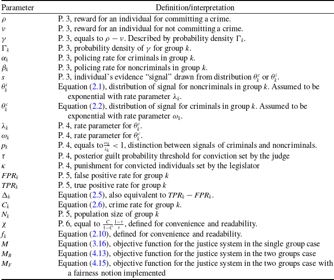


 Open access