Nomenclature
- AGC-T
-
attention-improved graph convolutional transformer
- CNN
-
convolutional neural network
- RNN
-
recurrent neural network
- LSTM
-
long short term memory network
- GRU
-
gated recurrent unit
- GCN
-
graph convolutional neural network
- ATM
-
air traffic management
- ATFM
-
air traffic flow management
- ANSP
-
air navigation service provider
- SVR
-
support vector regression
- RMSE
-
root mean square error
- MAE
-
mean absolute error
1.0 Introduction
The development of the civil aviation transportation industry is facing challenges such as air traffic congestion and low airspace operational efficiency. Accurate predictions of sector traffic can effectively assist air traffic management (ATM) departments in making more reasonable decisions and deploying air traffic flow management (ATFM) measures. With the significant increase in air transportation demand, the conflict between rapidly growing air traffic demand and the limited capacity of the air traffic management system has intensified, resulting in airspace congestion and flight delays. This phenomenon imposes higher requirements on ATM decision-making, which relies on accurate air traffic flow prediction (ATFP) [Reference Zhang, Hao and Gao1].
1.1 Air traffic flow prediction
From the perspective of prediction areas, ATFP can be classified into four levels: sector, route, waypoint and airport [Reference Murça and Hansman2]. Sector air traffic flow forecasting is critical to effective air traffic management and ensuring safe and orderly movement of aircraft through sectors, as sectors have limited capacity to handle flight missions within a given time [Reference Starita, Strauss, Fei, Jovanović, Ivanov, Pavlović and Fichert3]. Air traffic controllers manage flights on a sector-by-sector basis, so this paper focuses primarily on traffic flow prediction between sectors.
Sector flow forecasting [Reference Jiang, Luo, He and Gu4, Reference Jiang and Luo5] helps balance air traffic flows between different sectors. By predicting the expected demand and traffic volume for each flight segment, air traffic control officers (ATCOs) can adjust aircraft flows [Reference Hu, Xu, Bard, Chi and Gao6], distribute workload evenly and detect potential aircraft conflicts [Reference Jilkov, Ledet and Li7, Reference Matsuno, Tsuchiya, Wei, Hwang and Matayoshi8]. Research on ATFP can generally be divided into model-driven methods and data-driven methods [Reference Li, Zhang and Su9]. Model-driven methods address traffic issues by constructing mathematical or simulation models, while data-driven methods are mainly represented by time series algorithms [Reference Lin, Zhang and Liu10]. Time series algorithms treat air traffic flow as a time series [Reference Vardaro, Doan, Chandra and Mehta11] and predict future traffic by uncovering potential evolutionary patterns in historical time series data.
With the development of artificial intelligence, an increasing number of researchers have applied machine learning to sector traffic prediction [Reference Qiu and Li12], using methods such as support vector machines (SVM) [Reference Zhang, Jiang and Yang13] and shallow neural networks [Reference Wang, Liang and Delahaye14]. However, these approaches fail to account for the complex actual environment of air traffic, making it challenging to capture the spatial correlations between different regions, resulting in suboptimal performance. Considering the strong interdependence of air traffic flows in different regions, some researchers have encoded air traffic flows into traffic flow matrices (TFMs) and modeled spatiotemporal dependencies using convolutional neural networks (CNN) [Reference Lin, Zhang and Liu15] and long short-term memory (LSTM) networks [Reference Liu, Lin, Chen, Guo, Zhang and Jing16]. While these methods account for spatial correlations by discretising airspace and analysing spatial distributions and flow characteristics, they are unsuitable for predicting traffic in airspaces with irregular topologies. Additionally, they struggle with modeling long-term temporal dependencies.
1.2 Air traffic flow prediction model
Existing traffic prediction methods can be divided into two categories: model-driven and data-driven approaches.
1.2.1 Model-driven approach
The model-driven approach mainly explains the instantaneous and steady-state relationship between traffic volume, speed and density. This approach requires comprehensive and detailed system modeling based on prior knowledge. In reality, traffic data is affected by many factors, making it difficult to obtain an accurate traffic model. Existing models cannot accurately describe the changes in traffic data in complex real-world environments.
1.2.2 Data-driven approach
The data-driven method infers the trend of change based on the statistical laws of the data, and ultimately uses it to predict and evaluate traffic conditions. This method does not require analysis of the physical characteristics and dynamic behaviour of the traffic system and has high flexibility. One of the methods is the historical average model, which uses the average value of traffic volume in a historical time period as the prediction value. This method does not require any assumptions and is simple and fast to calculate, but it does not consider time characteristics and has low prediction accuracy.
As research in traffic prediction progresses, many methods with higher prediction accuracy have emerged, generally classified into parametric and non-parametric models. Parametric models use regression functions to process raw data, determine parameters and predict traffic based on the regression function. Common methods include time series models, linear regression models and Kalman filter models. The time series model fits a parametric model to the observed time series to predict future data [Reference Sun, Zhang and Ran17].
These traditional models are simple and computationally efficient but rely on assumptions that the system is static, failing to capture the nonlinearity and uncertainty of traffic data or mitigate the impact of stochastic events such as traffic incidents. Non-parametric models, such as support vector regression (SVR), overcome these limitations by learning statistical patterns from sufficient historical data without requiring prior assumptions.
In recent years, with the rapid development of deep learning [Reference Moravčík, Schmid, Burch, Lisý, Morrill, Bard, Davis, Waugh, Johanson and Bowling18], deep neural networks have gained attention for their ability to capture the dynamic characteristics of traffic data, achieving state-of-the-art performance. Recurrent neural networks (RNN) and their variants, such as LSTM and gated recurrent units [Reference Cho, Van Merriënboer and Gulcehre19] (GRU), effectively utilise recurrent mechanisms to learn temporal dependencies, producing favorable prediction results [Reference Van Lint, Hoogendoorn and Van Zuylen20]. In addition, other methods include but are not limited to natural language processing [Reference Sun, Zhang, Huang, Li, Zhang and Xu21, Reference Wu, Chen, Shen, Guo, Gao, Li, Pei and Long22], computer vision [Reference Cao, Zhu and Wang23, Reference Han, Wang and Guo24], recommendation systems, graph analysis [Reference Vo25] and traffic prediction.
However, these models consider only temporal features and ignore spatial dependencies, making them inadequate for predicting traffic constrained by airway or sector networks. Fully leveraging spatiotemporal correlations is critical for solving traffic prediction problems. To capture the spatial dependencies of air traffic flows, several end-to-end deep learning models have been proposed. However, these ATFP methods still have limitations.
Since air traffic controllers manage traffic on a sector-by-sector basis, using grid matrices for predicting traffic in airspace sectors with irregular topologies is inappropriate. Wu and Tan combined CNN and LSTM to design a feature fusion architecture [Reference Wu and Tan26] for short-term prediction, using 1D-CNN to capture spatial dependencies and two LSTMs to explore short-term variability and periodicity in traffic flow. Although these methods integrate CNNs for spatial dependency modeling and have advanced traffic prediction tasks, CNNs are fundamentally suited for Euclidean spaces, such as images or regular grids, and struggle with the complex topology of traffic networks, failing to inherently represent spatial dependencies.
The development of graph convolutional networks [Reference Kipf and Welling27] (GCNs) offers a promising solution to these challenges by capturing the structural features of graph networks. Zhao and Song [Reference Zhao, Song, Zhang, Liu, Wang, Lin, Deng and Li28] designed a temporal graph convolutional network (T-GCN) model, combining GCNs and GRUs. T-GCN uses GCNs to learn complex topologies and spatial dependencies and GRUs to model dynamic temporal changes in traffic data. Li et al. [Reference Li, Xiong, Chen, Lv, Hu, Zhu and Wang29] proposed a graph and attention-based long short-term memory network (GLA) to extract traffic flow temporal features by combining GCN with LSTM. Du et al. [Reference Du, Chen, Li, Cao and Lv30] combined GCN and GRU to predict traffic at multiple airports. Li et al. [Reference Li, Li, Chen, Yan, Lv and Du31] combined the attention-based temporal convolution module with graph convolution to establish a spatial complexity prediction model.
Some researchers have proposed neural network-based modeling approaches, such as CNNs, RNNs, and their variants (e.g. GRU and LSTM), for traffic prediction. While these methods have achieved notable improvements in training efficiency and prediction accuracy, their performance remains unsatisfactory.
To accurately predict sector traffic flows and describe the irregularity of sector spatial structures while mining spatiotemporal correlations in air traffic data, some neural network approaches (e.g. T-GCN) are tailored for the features of sector space and flight data. These methods typically model spatial and temporal features separately before combining them to analyse the complex dynamics and interdependencies of traffic flows. However, separate modeling often results in incomplete feature extraction and loose integration, leading to inaccurate or ineffective sector traffic predictions. To date, there is no perfect method that entirely relies on data extraction without considering spatial structural features.
Addressing the limitations of the aforementioned models, this study employs the Attention-improved Graph Convolutional Transformer (AGC-T) method, which considers various spatiotemporal dependencies using sectors as spatial nodes. Based on historical traffic data, the method incorporates multi-head attention mechanisms into the GCN model to effectively capture sector spatial structure features. By integrating GCN and transformer architectures, this approach is ultimately applied to sector traffic flow prediction tasks.
2.0 Preliminary
Currently, neural network methods, represented by models such as CNNs [Reference Lin, Zhang and Liu15], RNNs and their variants GRU and LSTM [Reference Liu, Lin, Chen, Guo, Zhang and Jing16] , have achieved significant success in research areas such as natural language processing (NLP) for textual information, automatic speech recognition (ASR) for audio information and computer vision [Reference Cao, Zhu and Wang23, Reference Han, Wang and Guo24] (CV) for image data. In practice, when the research object involves images or sequential data, methods like CNNs, RNNs or RNN variants such as GRUs and LSTMs can be employed. CNNs, designed to process two-dimensional data such as images, excel at extracting features through convolution-based operations. RNNs, on the other hand, are more suited for sequential data. However, RNNs are particularly effective only for short sequences, as they tend to lose information from earlier historical data in longer sequences [Reference Zhao, Song, Zhang, Liu, Wang, Lin, Deng and Li28]. Additionally, due to their architectural limitations, RNNs rely on sequential processing, where the output of the previous step is required before predicting the current step. This sequential dependency precludes parallel computation, significantly reducing efficiency when handling large datasets. In today’s era of information explosion and rapidly growing data volumes, these traditional data processing methods are increasingly inadequate to meet modern demands.
In fact, both images and sequence data are Euclidean space data with simple structures. When using CNN and RNN for processing, the input format must be fixed. That is, on the one hand, for images, the images need to be adjusted to a fixed size, and then convolution operations are performed to obtain features. On the other hand, text information also requires a fixed length and word vector size.
2.1 Transformer
The transformer model was first proposed by Vaswani et al. [Reference Vaswani, Shazeer, Parmar, Uszkoreit, Jones, Gomez, Kaiser and Polosukhin32] in a paper titled Attention Is All You Need published in 2017 and has been widely used in fields such as natural language processing and time series analysis as shown in Fig. 1. The model structure is shown in Fig. 2.

Figure 1. Comparison of three architectures: CNN, RNN and self attention.

Figure 2. Transformer model architecture.
2.1.1 Embedding
We cannot directly input the sector traffic data information into the encoder part of the transformer because the neural network cannot directly recognise data information. We need to convert the traffic data into a vector representation of a series of sequence data, that is, for a given traffic data sequence $\;\left( {{x_1},{x_2}, \ldots \ldots ,{x_n}} \right)\;$
for any
$\;\left( {{x_1},{x_2}, \ldots \ldots ,{x_n}} \right)\;$
for any ${x_t}\left( {t \in \left[ {1,2, \ldots \ldots ,n} \right]} \right)$
it is converted into the corresponding vector representation.
${x_t}\left( {t \in \left[ {1,2, \ldots \ldots ,n} \right]} \right)$
it is converted into the corresponding vector representation.
2.1.2 Positional encoding
The input of the transformer model is to map each word in a sequence to a high-dimensional space through an embedding layer, so that each word becomes a vector. However, since the transformer does not pay attention to the time sequence when processing data, the word embedding data alone does not contain position information. The position information of the sequence data needs to be added to the word embedding layer in advance. Since the transformer does not have the recursive structure of an RNN or a CNN, it is necessary to add position information to each word in an explicit way. Position encoding generates a fixed vector for each word position in the form of a function, and then adds it to the word embedding. Its function is to add position information to the input and enhance the model’s sensitivity to sequence order.
2.1.3 Encoder-decoder structure
The encoder structure is generally composed of multiple identical encoder layers stacked together, each of which contains a multi-head self-attention mechanism, a feed-forward neural network, residual connections and layer normalisation. After the encoder processes all layers, it outputs the context representation of each position, which will be passed to the decoder.
The decoder structure is also composed of multiple decoder layers, each of which mainly contains a multi-head self-attention mechanism, encoder-decoder attention and a feed-forward neural network, as well as residual connections and layer normalisation. The decoder finally outputs the predicted distribution, usually generating the probability distribution of each position of the target sequence through linear transformation and Softmax.
In general, when targeting prediction tasks, the encoder is responsible for extracting the global feature representation of the input sequence, while the decoder combines the feature representation of the encoder with the context information generated by itself to gradually generate the predicted target sequence.
2.2 GCN model — graph convolutional neural network
Models such as CNN are powerless for graph data without fixed structures, such as the molecular structure of substances in the field of biochemistry and social networks in the field of sociology. Currently, methods such as GNN, DeepWalk and Node2Vec are gradually gaining popularity, and the effect of GCN is more satisfactory.
GCN was first proposed in 2017 and has been successfully applied to image and document classification and unsupervised learning.
Based on the idea of transforming graph signals in the Fourier domain in graph signal processing, for graph structure data with nodes, given the adjacency matrix A (representing the connection relationship between nodes, in an undirected graph, if the nodes are connected, the corresponding element is 1, otherwise the element is 0; in a directed graph, the corresponding element is 1 only when there is active directionality, otherwise the element is 0) and the feature matrix X (representing the feature dimension matrix of the node), the GCN model aggregates the first-order neighbourhood information (other nodes directly connected to the node) of each node in the graph by designing a filter function $\hat A$
to simulate the effect of convolution. By multiplying the filter function
$\hat A$
to simulate the effect of convolution. By multiplying the filter function $\hat A$
each node in the graph can aggregate the feature information of the nodes in its own field, thereby completing the extraction of spatial features.
$\hat A$
each node in the graph can aggregate the feature information of the nodes in its own field, thereby completing the extraction of spatial features.
 \begin{equation}{H^{l + 1}} = \sigma \left( {{{\hat D}^{ - \frac{1}{2}}}{A^I}{{\hat D}^{ - \frac{1}{2}}}{H^l}{W^l}} \right)\end{equation}
Among them, ${H^{l + 1}}$
represents the output, with a shape of
${H^{l + 1}}$
represents the output, with a shape of $N \times C'$
where is the number of N nodes and
$N \times C'$
where is the number of N nodes and $C'$
is the feature dimension of the output.
$C'$
is the feature dimension of the output. $\;{A^I} = A + {I_N}$
represents the adjacency matrix with added self-connection (considering the characteristics of the node itself), and
$\;{A^I} = A + {I_N}$
represents the adjacency matrix with added self-connection (considering the characteristics of the node itself), and ${I_N}$
represents the identity matrix. D is the degree matrix, where the diagonal elements represent the degree of each node (that is, the number of edges connected to the node); since the adjacency matrix
${I_N}$
represents the identity matrix. D is the degree matrix, where the diagonal elements represent the degree of each node (that is, the number of edges connected to the node); since the adjacency matrix ${A^I}$
adds the node’s own connection, then considers this factor and D transforms into
${A^I}$
adds the node’s own connection, then considers this factor and D transforms into $\hat D$
;
$\hat D$
; ${\hat D^{ - \frac{1}{2}}}{A^I}{\hat D^{ - \frac{1}{2}}}$
is a normalisation operation to ensure that the original distribution of the feature matrix
${\hat D^{ - \frac{1}{2}}}{A^I}{\hat D^{ - \frac{1}{2}}}$
is a normalisation operation to ensure that the original distribution of the feature matrix ${H^l}$
is maintained during the information transmission process, while preventing the node features from having large distribution differences. This not only makes the data more comparable, but also maintains the connection between the data.
${H^l}$
is maintained during the information transmission process, while preventing the node features from having large distribution differences. This not only makes the data more comparable, but also maintains the connection between the data. $\;{H^l}$
represents the input of the lth layer, which is the feature matrix X for the input layer, with a shape of
$\;{H^l}$
represents the input of the lth layer, which is the feature matrix X for the input layer, with a shape of $N \times C$
, where C is the feature dimension.
$N \times C$
, where C is the feature dimension. $\;{W^l}$
represents the training weight parameter of the lth layer, with a shape of
$\;{W^l}$
represents the training weight parameter of the lth layer, with a shape of $N \times C'$
.
$N \times C'$
. $\sigma \left( \bullet \right)$
represents the nonlinear activation function, which is used to map the features of the nodes in the graph to between 0 and 1.
$\sigma \left( \bullet \right)$
represents the nonlinear activation function, which is used to map the features of the nodes in the graph to between 0 and 1.
3.0 Methodology
This section introduces the basic idea of sector traffic flow prediction and elaborates on the structure of the AGC-T model.
3.1 Predictive modeling and visualisation
The basic modeling idea of sector traffic flow prediction is to model based on the feature matrix X of the previous P (indicating the past) time steps of the sector historical traffic data and the currently known sector spatial structure S, and to perform deep learning training on the mapping function f, and the sector traffic flow value Y in the future period F. Its basic function is shown in Equation (2).
 \begin{equation}\left[ {{Y_{t + 1}}, \ldots \ldots ,{Y_{t + F}}\left] { = f} \right[S\left( {{X_{t - P}}, \ldots \ldots .,{X_{t - 1}},{X_t}} \right)} \right]\end{equation}
Based on this idea of modeling [Reference Zhang, Xu, Zhang, Jiang, Alam and Xue33], the spatial structural relationship between sectors can be converted into the adjacency matrix ${A^{n \times n}}$
shown in Equation (3). Each row of the matrix represents a complete flight route passing through a specified sector, and each column of the matrix represents the time dimension.
${A^{n \times n}}$
shown in Equation (3). Each row of the matrix represents a complete flight route passing through a specified sector, and each column of the matrix represents the time dimension.
 \begin{equation} A = \left[ {\begin{array}{c@{\quad}c@{\quad}c@{\quad}c}{{a_{11}}} & {}{{a_{12}}} {}& \cdots & {}{{a_{1n}}}\\{{a_{21}}} {}&{} & {}{} {}& \vdots \\ \vdots {}&{} {} & \ddots & {}{}\\{{a_{n1}}} {}& \cdots & {}{} {}&{{a_{nn}}}\end{array}} \right]\end{equation}
Among them, n represents the number of sectors and ${a_{ij}}$
represents the directed connectivity between sectors.
${a_{ij}}$
represents the directed connectivity between sectors.
 \begin{equation}X = \left[ {\begin{array}{c@{\quad}c@{\quad}c@{\quad}c}{\left( {{s_{11}},{w_{11}}} \right)} & {}{\left( {{s_{12}},{w_{12}}} \right)} & {} \cdots {}& {\left( {{s_{1t}},{w_{1t}}} \right)}\\{\left( {{s_{21}},{w_{21}}} \right)}& & {}{} {} \vdots & {}{}\\ \vdots & {}{} {}& \ddots {} {}\\{\left( {{s_{n1}},{w_{n1}}} \right)} {}& \cdots & & {}{} {}{\left( {{s_{nt}},{w_{nt}}} \right)}\end{array}} \right]\end{equation}
The matrix X shown in Equation (4) represents the feature set of the sector at different time intervals, where ${S_{ij}}$
represents the planned or actual traffic of the sector, respectively. We will use the actual traffic to learn and train the mapping function. For details, refer to the Description of Sector and Dataset section later in this article. t represents the length of the historical time series, and
${S_{ij}}$
represents the planned or actual traffic of the sector, respectively. We will use the actual traffic to learn and train the mapping function. For details, refer to the Description of Sector and Dataset section later in this article. t represents the length of the historical time series, and ${w_{ij}}$
represents the weight characteristics of different sectors showing periodic regularity. The air traffic field usually presents regular characteristics with daily and weekly periods.
${w_{ij}}$
represents the weight characteristics of different sectors showing periodic regularity. The air traffic field usually presents regular characteristics with daily and weekly periods.
 \begin{equation} Y = \left[ {\begin{array}{*{20}{l}}{{y_{t + 1}},{y_{t + 2}}, \ldots \ldots .,{y_{t + F}}}\end{array}} \right]\end{equation}
The deeply trained model is able to predict traffic values for future time periods F.
3.2 AGC-T prediction model
In order to make traffic prediction more accurately, the AGC-T model is proposed. The model mainly includes an input layer involving embedded coding, a GCN layer based on multi-layer attention, a transformer layer based on time series position coding, and an output layer for decoding and restoring traffic prediction data. The main architecture of the model is shown in Fig. 3.

Figure 3. AGC-T model architecture.
The process of applying the historical traffic data of the sector to the entire model is as follows: the input layer first receives the spatial structure data and historical traffic data obtained after preliminary processing, extracts spatial features through the graph convolution improved by multi-head attention, and the output result sequence is encoded and input into the transformer layer to capture the temporal correlation in the data, and finally outputs the feature results through the output layer.
After the overall improvement plan, the model can complete the extraction of spatial and temporal features in the data and apply them to the final accurate traffic prediction.
3.2.1 Multi-head GCN layer
In order to adapt to the multi-head attention in transformer, multi-head operations are also performed on GCN, which allows the convolution operation in the model to obtain features of different dimensions to enhance the model’s transmission and modeling capabilities, which is beneficial to the final prediction output and can avoid the data feature dimension problem that may occur when the two are combined. The entire multi-head attention graph convolution layer is based on the following equations:
 \begin{equation} H = Concatenate\left[ {\sigma \left( {{D^{ - \frac{1}{2}}}{A_1}{D^{ - \frac{1}{2}}}X{W_1}} \right),\sigma \left( {{D^{ - \frac{1}{2}}}A_2^{ - \frac{1}{2}}X{W_2}} \right), \ldots \ldots ,\sigma \left( {{D^{ - \frac{1}{2}}}A_n^{ - \frac{1}{2}}X{W_n}} \right)} \right]\end{equation}
 \begin{equation}{A_n} = Softmax\left( {{E_n}} \right)\end{equation}
 \begin{equation}{E_{ij}} = ReLU\left( {a_n^T\left[ {{W_n}{X_i}{\rm{K}}{W_n}{X_j}} \right]} \right).\end{equation}
Among them, $H$
represents the output of the multi-head GCN layer,
$H$
represents the output of the multi-head GCN layer, $n$
represents the number of attention heads,
$n$
represents the number of attention heads, ${A_n}$
represents the attention weight matrix of the
${A_n}$
represents the attention weight matrix of the $n$
-th attention head,
$n$
-th attention head, $D$
is the degree matrix considering its own connection,
$D$
is the degree matrix considering its own connection, $X$
represents the feature matrix,
$X$
represents the feature matrix, ${W_n}$
represents the linear transformation weight matrix of the
${W_n}$
represents the linear transformation weight matrix of the $n$
-th attention head,
$n$
-th attention head, $\sigma \left( \cdot \right)$
represents the activation function,
$\sigma \left( \cdot \right)$
represents the activation function, ${E_{ij}}$
represents the attention weight between
${E_{ij}}$
represents the attention weight between $i,j$
nodes, then
$i,j$
nodes, then ${E_n}$
represents the set of
${E_n}$
represents the set of ${E_{ij}}$
, which ensures that the sum of the attention weights of each node is 1 through the Softmax [Reference Zhang, Xu, Zhang, Jiang, Alam and Xue33] operation,
${E_{ij}}$
, which ensures that the sum of the attention weights of each node is 1 through the Softmax [Reference Zhang, Xu, Zhang, Jiang, Alam and Xue33] operation, ${X_i},{X_j}$
represents the feature vectors between
${X_i},{X_j}$
represents the feature vectors between $i,j$
nodes respectively, Krepresents the concatenation operation of the vector, and
$i,j$
nodes respectively, Krepresents the concatenation operation of the vector, and $ReLU\left( \cdot \right)$
[Reference Zhang, Xu, Zhang, Jiang, Alam and Xue33] represents the activation function.
$ReLU\left( \cdot \right)$
[Reference Zhang, Xu, Zhang, Jiang, Alam and Xue33] represents the activation function.
3.2.2 Transformer based on temporal position encoding
Since the sector traffic data contains strong time series information and periodic information, which has a great impact on model training and the final output, time position encoding is added after completing the high-dimensional embedding encoding of the traffic data. Assuming that the input matrix $X \in {R^{n \times d}}$
represents the
$X \in {R^{n \times d}}$
represents the $d$
dimensional embedding of
$d$
dimensional embedding of $n$
words in a sequence. The position encoding is used to generate a position embedding matrix
$n$
words in a sequence. The position encoding is used to generate a position embedding matrix $P \in {R^{n \times d}}$
with the same shape as
$P \in {R^{n \times d}}$
with the same shape as $X$
, and the output is
$X$
, and the output is $X + P$
. The formula for the elements on the
$X + P$
. The formula for the elements on the $i$
th row,
$i$
th row, $2j$
th column and
$2j$
th column and $2j + 1$
th column of the matrix
$2j + 1$
th column of the matrix $P$
is as follows:
$P$
is as follows:
 \begin{equation}{P_{ij}} = \left( {\begin{array}{*{20}{l}}{{\rm{sin}}\left( {i/{{1000}^{2j/d}}} \right)} {}{{\rm{if\;}}j\;{\rm{is\;even}}}\\[8pt]{{\rm{cos}}\left( {i/{{1000}^{2j/d}}} \right)} {}{{\rm{if\;}}j\;{\rm{is\;odd}}}\end{array}} \right.\end{equation}
3.2.3 Normalisation
During model training and prediction, sample data will be normalised to avoid gradient vanishing or gradient exploding problems during model training and to improve visualisation.
As shown in Fig. 4, when normalising sequences of the same length, we usually choose to normalise the same feature of different samples, that is, BatchNorm. For some samples of variable length sequences (i.e. samples with different lengths), layer normalisation (LayerNorm) [Reference Ba, Kiros and Hinton34] has better adaptability. In order to adapt to the normalisation method in transformer, the normalisation operations in this study all use layer normalisation.

Figure 4. Normalisation type comparison.
3.2.4 Loss function
In order to effectively prevent overfitting during model training, the L2 regularisation term is added to the loss function $MSE\;$
(mean squared error). The formula is as follows:
$MSE\;$
(mean squared error). The formula is as follows:
 \begin{equation}loss\left( w \right) = \mathop \sum \limits_{i = 1}^m {({\hat y_i} - {y_i})^2} + \lambda \cdot \mathop \sum \limits_{j = 1}^n w_j^2\end{equation}
Among them,
-
• ${\hat y_i}$
represents the predicted flow value;
${\hat y_i}$
represents the predicted flow value; -
•
${y_i}$
represents the actual flow value; -
•
$\lambda $
represents the L2 regularisation coefficient, which is used to control the strength of the regularisation term; -
•
$w$
represents the training weight value; -
•
$loss\left( \bullet \right)$
represents the final loss output value.


Overfitting is usually caused by the model being too complex, too few training samples, etc. The complexity of the training model is determined by the number and size range of the training weight values, so by reducing the number and size range, the complexity of the model can be reduced, thus effectively solving the overfitting problem.
3.2.5 Evaluation indicators
The experimental results of the AGC-T model are evaluated using indicators such as $RMSE\;$
(root mean square error),
$RMSE\;$
(root mean square error), $MAE\;$
(mean absolute error), and
$MAE\;$
(mean absolute error), and ${R^2}\;$
(determination coefficient). The formula is as follows:
${R^2}\;$
(determination coefficient). The formula is as follows:
 \begin{equation} RMSE = \sqrt {{1 \over n}\mathop \sum \limits_1^n {{({{\hat y}_i} - {y_i})}^2}} ,\end{equation}
 \begin{equation} MAE = {1 \over n}\mathop \sum \limits_1^n \left| {{{\hat y}_i} - {y_i}} \right|\end{equation}
 \begin{equation} {R^2} = 1 - {{\mathop \sum \nolimits_1^n {{({{\hat y}_i} - {y_i})}^2}} \over {\mathop \sum \nolimits_1^n {{({y_i} - \bar y)}^2}}}.\end{equation}
Among them,
-
•
${\hat y_i}$
represents the predicted flow value; -
•
${y_i}$
represents the actual flow value; -
•
$\bar y$
represents the average of the actual flow values; -
•
$n$
represents the number of samples.


 $RMSE$
and
$RMSE$
and $MAE$
are used to measure the error between the model prediction result and the actual flow value. The smaller the value, the better the prediction effect.
$MAE$
are used to measure the error between the model prediction result and the actual flow value. The smaller the value, the better the prediction effect. ${R^2}$
represents the degree of fit of the model to the data. The closer it is to 1, the better the model can fit the data and make more accurate predictions.
${R^2}$
represents the degree of fit of the model to the data. The closer it is to 1, the better the model can fit the data and make more accurate predictions.
4.0 Verification and Results
This section first introduces the experimental data set and selects key regional sectors in the high-altitude airspace in central and southern China for case studies. Then, a graph structure is constructed based on the spatial distribution of each sector in the airspace. In order to verify the effectiveness and accuracy of the model, AGC-T is compared with five baseline models at different time steps, and evaluation indicators are used to judge the pros and cons of the experimental results.
4.1 Dataset settings
Automatic dependent surveillance – broadcast (ADS-B) data is used as the basic data for the experiment. ADS-B is based on the global navigation satellite system and can provide relatively comprehensive data including flight ID, sector name, sector entry point, sector exit point, planned and actual sector entry and exit time, etc. However, in fact, there is not much available and effective data, so the initial data needs to be preprocessed to form a usable data set.
4.1.1 Sector and dataset description
The data mainly comes from 11 regional sectors located in the central and southern regions of China. They are key hubs connecting many airports. Compared with other airspaces, these sectors have higher traffic and play an extremely important role in the air traffic system.
Figure 5 is a three-dimensional spatial position distribution map of these sectors in the high-altitude airspace of the central and southern regions. It can be clearly seen that the relative position relationship between the 11 sectors has large differences in structure, horizontal range and height.

Figure 5. Spatial location distribution of 11 regional sectors in central and southern China.
This study uses the ADS-B data set from March 1 to March 31, 2019 and preprocesses it to meet the model input requirements. The data set contains 215,014 flight records in 11 regional sectors.
The flow value data, that is, the occupancy of the sector in a specified period, is calculated by the actual entry and exit time of the sector. Due to the abnormal data generated by the inconsistent correction of the entry and exit time of the sector, the planned flow is used instead of the actual flow. If there is still a conflict, the data is discarded. Finally, a data set of 211,549 flight records containing valid sector flow data was obtained. The flow data in the data set is counted separately according to the time periods of 15 min, 30 min and 1 h as needed for model training and prediction.
4.1.2 Data preprocessing
According to the spatial position relationship of the 11 sectors in the central and southern regions, as shown in Fig. 6(a), we can get the directed network topology structure $S = \left( {N,E} \right)$
between the sectors, as shown in Fig. 6(b), where
$S = \left( {N,E} \right)$
between the sectors, as shown in Fig. 6(b), where $N$
represents the node (sector),
$N$
represents the node (sector), $E$
represents the edge (sector directed traffic flow) and thus we get the schematic diagram of the adjacency relationship between sectors, as shown in Fig. 6(c). For example, it can be seen from Fig. 6 that sector ZGGG34 and sector ZGGG02 form a high-low sector, that is, sector ZGGG02 is located on the right side of the entire sector network structure and plays an important role in managing route traffic flow. Based on this connection relationship, the connection relationship between sectors is represented by the adjacency matrix
$E$
represents the edge (sector directed traffic flow) and thus we get the schematic diagram of the adjacency relationship between sectors, as shown in Fig. 6(c). For example, it can be seen from Fig. 6 that sector ZGGG34 and sector ZGGG02 form a high-low sector, that is, sector ZGGG02 is located on the right side of the entire sector network structure and plays an important role in managing route traffic flow. Based on this connection relationship, the connection relationship between sectors is represented by the adjacency matrix $A$
, and used as the input of the GCN layer together with the feature matrix
$A$
, and used as the input of the GCN layer together with the feature matrix $X$
.
$X$
.

Figure 6. Sector network structure diagram generated based on sector spatial location.
After preliminary processing of the original data, time series data of different step lengths in different time periods can be obtained for 11 sectors. However, before inputting the model, the traffic data needs to be converted into tokens that the model can recognise and train, and time series features need to be added. To this end, the following work needs to be done.
First, similar to natural language text processing, each word is regarded as a token. Here, each traffic data is regarded as a ‘word’, and the time series composed of them is mapped to an embedding vector through the embedding layer. At the same time, since the time of traffic data can be introduced into the model as a feature, we add time position encoding to enable the model to capture time correlation from the data, thereby achieving better prediction. For the specific addition method, refer to Equation (9).
4.2 Experimental setup
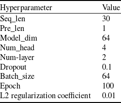
The hyperparameter settings of the AGC-T model are shown in Table 1.
Table 1. AGC-T model hyperparameter settings

In order to evaluate the performance of the AGC-T model, it is compared with five baseline models:
-
1. HA (historical average): This method predicts future traffic flow by averaging historical traffic data.
-
2. ARIMA (auto regressive integrated moving average): This technique is primarily used for non-stationary time series data.
-
3. SVR: This uses support vector machines for regression tasks.
-
4. GRU: This is a variant of recurrent neural networks designed to address vanishing or exploding gradient problems in RNNs.
-
5. GCN: This processes graph data and extracts features from graph nodes.
In the experiment, the ZGGGAR02 sector was used as the experimental object, 70% of the data was used as a training set, the test data corresponding to the prediction period was assigned to the test set and the remaining data was assigned to the validation set. In order to ensure the accuracy and research ability of the experiment as much as possible, the traffic forecast for the corresponding future time period was carried out for the historical traffic data of different time periods. The final prediction range was the single week (March 25, 2019–March 31, 2019) and the single day (March 31, 2019) of the data set, and the model prediction performance was evaluated. For example: if 15 min of historical time traffic data is taken, the future 15 min of traffic is predicted for the last week and the last day of the data set. At this time, 672 data of the last week and 96 data of the last day are used as test sets, respectively. Based on this principle, the same prediction is made for 30 min and 1 h of historical traffic data, respectively.
4.3 Experimental results
According to the experimental data settings and the settings of various experimental parameters, the model training and prediction tasks were carried out, respectively, and the following experimental results were obtained.
4.3.1 Single-day forecast results based on different historical time data
Based on the historical traffic data of 15 min, 30 min and 1 h, the daily traffic conditions of the ZGGGAR02 sector on March 31, 2019 were predicted. The comparison between the predicted value and the actual value is shown in Fig. 7.

Figure 7. ZGGGAR02 sector daily traffic forecast and actual value.
Figure 7(a), (b), (c) show the single-day prediction results of the AGC-T model based on 15-min, 30-min and 1-h historical traffic data, respectively. The model prediction effect based on 15-min data is the best, because the data samples based on the 15-min period are the most in the same data, so the model training effect is better and can have better prediction performance. In addition, it can be seen that the prediction effect of the AGC-T model for extreme data such as local maximum and minimum values is slightly poor, which is mainly due to the stability requirements of the model and the insufficient amount of extreme data.
Figure 8(a), (b) and (c) show the residual results of the AGC-T model sector single-day prediction value and the true value. The residual value of the model prediction based on 15-min data is the smallest, and as the amount of training data decreases, the residual value gradually increases.

Figure 8. Residual value of daily flow prediction in ZGGGAR02 sector.
Figure 9(a), (b) and (c), respectively, show the training loss of the AGC-T model under the sector single-day prediction task. The overall training iteration of the AGC-T model is fast. As the amount of data decreases, more rounds of training are required to obtain a stable prediction model.

Figure 9. Training loss of ZGGGAR02 sector daily traffic prediction model.
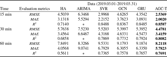
Based on the sector single-day traffic prediction task of historical traffic data in different time periods, the AGC-T model and other five baseline models are used to make predictions at different time granularities, and the prediction performance of the model is evaluated by $RMSE$
,
$RMSE$
, $MAE$
and
$MAE$
and ${R^2}$
, respectively. The results are shown in Table 2 and * indicates that the value is so small that it can be ignored, indicating that the prediction effect of the model is poor.
${R^2}$
, respectively. The results are shown in Table 2 and * indicates that the value is so small that it can be ignored, indicating that the prediction effect of the model is poor.
Table 2. Sector single-day forecast performance of AGC-T model and baseline model

The AGC-T model outperforms other models in the sector single-day traffic prediction task. In the 15-min traffic prediction task, compared with the GCN model that only considers spatial features, the AGC-T model’s $RMSE$
,
$RMSE$
, $MAE$
and
$MAE$
and ${R^2}$
increased by 45.16%, 46.78% and 2.63%, respectively, indicating that the model can effectively capture the spatial dependency of complex data; compared with the GRU model that only considers temporal features, the AGC-T model’s
${R^2}$
increased by 45.16%, 46.78% and 2.63%, respectively, indicating that the model can effectively capture the spatial dependency of complex data; compared with the GRU model that only considers temporal features, the AGC-T model’s $RMSE$
,
$RMSE$
, $MAE$
and
$MAE$
and ${R^2}$
increased by 41.74%, 35.27% and 1.20%, respectively, which can better capture the temporal dependency of time series data. For the 30-min and 60-min prediction tasks, the AGC-T model also performed well.
${R^2}$
increased by 41.74%, 35.27% and 1.20%, respectively, which can better capture the temporal dependency of time series data. For the 30-min and 60-min prediction tasks, the AGC-T model also performed well.
4.3.2 Single-week forecast results based on different historical time data
Based on the historical traffic data of 15 min, 30 min and 1 h, the weekly traffic conditions of the ZGGGAR02 sector from March 1, 2019 to March 31, 2019 were predicted. The comparison between the predicted value and the actual value is shown in Fig. 10.

Figure 10. ZGGGAR02 sector weekly traffic forecast and actual value.
Figure 10(a), (b), (c) show the weekly prediction results of the AGC-T model based on 15-min, 30-min and 1-h historical traffic data, respectively. The model prediction effect based on 15-min data is the best. At the same time, due to the lack of traffic data during the peak period of the sector, the AGC-T model has a poor prediction effect on the peak traffic. Similarly, due to the stability requirements of the model and the lack of extreme data, AGC-T’s prediction performance for local extreme values is slightly poor. Better prediction performance requires further optimisation of the model and the addition of more extreme data.
Figure 11(a), (b), and (c) show the residual results of the AGC-T model sector single-week prediction value and the true value. The model prediction residual value based on 15-min data is the smallest. Except for the large residual value during the peak traffic period, the overall residual value is within the prediction error.

Figure 11. Residual value of single-week traffic forecast for ZGGGAR02 sector.
Figure 12(a), (b), (c), respectively, show the training loss of the AGC-T model under the sector single-week prediction task. The overall training iteration of the AGC-T model is fast. As the amount of data decreases, more rounds of training are required to obtain a stable prediction model.

Figure 12. Training loss of single-week traffic prediction model for ZGGGAR02 sector.
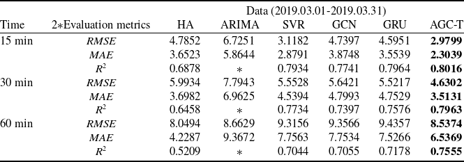
Based on the sector single-week traffic prediction task of historical traffic data in different time periods, the AGC-T model and other five baseline models are used to make predictions at different time granularities, and the prediction performance of the model is evaluated by $RMSE$
,
$RMSE$
, $MAE$
and
$MAE$
and ${R^2}$
, respectively. The results are shown in Table 3 and * indicates that the value is so small that it can be ignored, indicating that the prediction effect of the model is poor.
${R^2}$
, respectively. The results are shown in Table 3 and * indicates that the value is so small that it can be ignored, indicating that the prediction effect of the model is poor.
Table 3. Sector single-week forecast performance of AGC-T model and baseline model

The AGC-T model outperforms other models in the sector single-week traffic prediction task. In the 15-min traffic prediction task, compared with the GCN model that only considers spatial features, the AGC-T model’s $RMSE$
,
$RMSE$
, $MAE$
and
$MAE$
and ${R^2}$
increased by 37.12%, 40.54% and 3.55%, respectively, indicating that the model can effectively capture the spatial dependency of complex data; compared with the GRU model that only considers temporal features, the AGC-T model’s
${R^2}$
increased by 37.12%, 40.54% and 3.55%, respectively, indicating that the model can effectively capture the spatial dependency of complex data; compared with the GRU model that only considers temporal features, the AGC-T model’s $RMSE$
,
$RMSE$
, $MAE$
and
$MAE$
and ${R^2}$
increased by 35.15%, 35.17% and 0.65%, respectively, which can better capture the temporal dependency of time series data. For the 30-min and 60-min prediction tasks, the AGC-T model also performed well.
${R^2}$
increased by 35.15%, 35.17% and 0.65%, respectively, which can better capture the temporal dependency of time series data. For the 30-min and 60-min prediction tasks, the AGC-T model also performed well.
Additionally, the AGC-T model does not include additional dropout layers. However, the results demonstrate that the AGC-T model outperforms other models in all aspects of performance. This is because the original transformer architecture already incorporates multiple dropout layers. These layers randomly ‘drop out’ certain neurons during training, reducing the model’s dependency on specific features, thereby preventing overfitting and enhancing the model’s generalisation ability. This may also be the reason why the ${R^2}$
of the AGC-T model is slightly worse than other models.
${R^2}$
of the AGC-T model is slightly worse than other models.
4.4 Discussion and summary
The AGC-T model proposed in this study still has certain shortcomings. First of all, considering that traffic prediction may be performed for sectors with different spatial structures, the AGC-T model still needs to rebuild the graph structure and retrain the network. This is because the model still uses the architecture of the GCN model to obtain spatial features by constructing a sector adjacency matrix, and does not completely abandon the method of constructing the graph structure. When traffic prediction is required for other sectors, the graph structure must be reconstructed, which is not conducive to quickly predicting sector traffic. Modeling the spatial structure of sectors must fully consider the influencing factors. Not only can it not solve the problem of possible feature loss or incomplete feature extraction caused by model separation and construction and then combination, but the prediction model can only be applied to a specific sector with a certain spatial structure. Once the sector structure changes or traffic flow prediction is performed for other sectors, it must be re-modeled based on the new spatial structure, indicating that the AGC-T model combined with the graph structure is still not the best solution; secondly, due to the ‘end-to-end’ prediction method of traffic data, it is impossible to accurately analyse the impact of a major factor of traffic change. For example, the impact of weather conditions on sector traffic flow is significant, but the AGC-T model cannot quantify the impact of individual weather conditions on traffic flow, resulting in air traffic controllers may not be able to take specific traffic management measures for a certain factor.
However, this study provides the following contributions. First, the AGC-T model can make a single-step prediction of traffic flow between sectors based on traffic data in different historical time periods, showing excellent performance; secondly, the attention mechanism can capture the graph structure information with sectors as nodes, significantly improving the prediction accuracy; finally, the parallel training structure based on transformer greatly shortens the rounds (epochs) of the training model and improves the training efficiency. Therefore, the AGC-T model can assist the air navigation service providers in making decisions and issue more scientific and reasonable control strategies to achieve the goal of effectively managing traffic and reducing workload.
5.0 Conclusion and Future Work
Deep learning models can learn and train based on data, and learn temporal and spatial features from data. This non-traditional mathematical modeling method greatly reduces the difficulty of air traffic flow prediction. Today, with the rapid development of society and the rapid increase in data volume, it provides a good opportunity for data-driven machine learning methods, which will further improve the accuracy and effectiveness of air traffic flow prediction. The AGC-T model proposed in this study can be used for accurate and real-time prediction of traffic flow between sectors. The traffic flow within a sector is not only affected by the number of planned flights, but also by the complexity of the airspace within the sector. To solve this problem, our model integrates a multi-head attention mechanism into GCN, which effectively captures the topological structure of the sector and focuses on key nodes. In addition, the transformer model is combined to capture the temporal dynamics of node attributes, thereby extracting important spatiotemporal features from the data. Through comprehensive comparison with five baseline models, our proposed method shows superior performance in all evaluation indicators. The AGC-T model has also been shown to be very proficient in accurately predicting the length of multiple input sequences, which is mainly due to the applicability of the transformer model to massive data and its powerful feature extraction capabilities. This not only makes up for the insufficient utilisation of large amounts of data in classic traffic flow prediction methods, but also eliminates the need to construct various complex parameters for different actual situations, greatly improving prediction efficiency and achieving substantial progress.
Furthermore, the rapid development of the civil aviation industry has not only accumulated a large amount of effective data through the integration of static and dynamic data such as flight schedules, flight dynamics and fleet information through civil aviation data analysis systems, but also enhanced the capabilities of data extraction technology due to the development of a growing number of artificial intelligence platforms. All of these factors have provided realistic conditions for the feasibility of implementing the AGC-T model. All results highlight the effectiveness of the AGC-T method in predicting sector traffic flow and demonstrate its great potential for practical application in the aviation field. The research done in this paper still has many shortcomings. In future work, further research can be carried out by combining other factors such as weather factors, which may improve the prediction performance of the model.
Acknowledgements
This research was supported by the National Key R&D Program of China (No.2022YFB2602401), the National Key R&D Program of China (No.2022YFB2602403) and the National Natural Science Foundation of China (Grant Nos. U2033203).
Competing interests
The authors declare that they have no known competing financial interests or personal relationships that could have appeared to influence the work reported in this paper.