

The normalized scores  $s^{*}_1, s^{*}_2,\ldots, s^{*}_n$ are exchangeable random variables for the fixed $n$, i.e., n-exchangeable or finite exchangeable. Their distribution depends on $n$, and their correlation is a function of $n$. Therefore, if they are a segment of the infinite sequence $s^{*}_1, s^{*}_2,\dots$, then they are not exchangeable, i.e., not infinite exchangeable and also not stationary. Accordingly, Berman's theorem [Reference Berman2] (Theorem 2.1 in the article) and Theorems 4.5.2. and 5.3.4. from [Reference Leadbetter, Lindgren and Rootzén5], which hold for stationary sequences, cannot be used in the proofs of Results 2.1. and 2.2. However, from Theorem 1 presented and proved below, for $P(X_{ij}=1/2)=p\in [1/3, 1)$ or $p=0$, Results 2.1. and 2.2. follows, and therefore, so do the follow-up Corollaries 2.1. and 2.2.
Let  ${I_{j}^{(n)}=I(s_{j}^{*}\gt x_n(t))}$, where we choose $x_n(t)=a_n t+b_n$, in which $a_n$ and $b_n$ are as defined in equation (1) in the article:
 \[ a_n=(2 \log n)^{-{1}/{2}},\quad b_n=(2\log n)^{{1}/{2}}-\tfrac{1}{2}(2 \log n)^{-{1}/{2}}(\log\log n+\log 4\pi). \]
Set  ${S_n= I_{1}^{(n)}+ I_{2}^{(n)}+\cdots + I_{n}^{(n)}}$.
We prove the following result.
Theorem 1. For  $p=0$ or ${p \in [{1}/{3}, 1)}$ and a fixed value of $k$,
$k$,  $\lim _{n\rightarrow \infty }P(S_n=k)=e^{-\lambda (t)}({\lambda (t)^k}/{k!})$, $\lambda (t)= e^{-t}$.
For  $p=0$ or ${p \in [{1}/{3}, 1)}$, Results 2.1. and 2.2. follow from Theorem 1, since ${P(s^{*}_{(n-j)}\leq x_n)=P(S_n\leq j)}$, and therefore
 \[ {\lim_{n\rightarrow \infty} P(s^{*}_{(n-j)}\leq x_n)= \lim_{n\rightarrow \infty}P(S_n\leq j)}=e^{{-}e^{{-}t}}\sum_{k=0}^j \frac{e^{{-}tk}}{k!}. \]
Remark 1. It remains an open problem if Theorem 1 holds also for  ${p \in (0, {1}/{3})}$.
Proof. (Theorem 1) The result follows from Assertions presented below. Set
 \[ \pi_{i}^{(n)}=P(I_{i}^{(n)}=1),\quad W_{n}=\sum_{i=1}^{n}I_{i}^{(n)},\quad \lambda_n=E(W_n)=\sum_{i=1}^{n}\pi_{i}^{(n)}. \]
Assertion 1.
 \begin{equation} d_{{\rm TV}}({L}(W_n), {\rm Poi}(\lambda_n))\leq \frac{1-e^{\lambda_n}}{\lambda_n}(\lambda_n-{\rm Var}(W_n)) =\frac{1-e^{\lambda_n}}{\lambda_n}\left(\sum_{i=1}^{n}(\pi_{i}^{(n)})^2- \sum_{i\neq j}{\rm Cov} (I_{i}^{(n)}, I_{j}^{(n)})\right), \end{equation}
where  ${d_{{\rm TV}}({L}(W_n), {\rm Poi}(\lambda _n))}$ is the total variation distance between distributions of $W_n$ and Poisson distribution with mean $\lambda _n$.
Assertion 2.
 \begin{equation} \pi_{1}^{(n)}=P(s_{1}^{*}\gt x_n(t))\sim 1-\Phi(x_n(t)), \end{equation}
where  ${c_n\sim k_n}$ means ${\lim _{n\rightarrow \infty } c_n/k_n=1}$.
Assertion 3.
 \begin{equation} {\lim_{n\rightarrow \infty}n \pi_{1}^{(n)}=\lim_{n\rightarrow \infty}n P(s_{1}^{*}\gt x_n(t))=\lambda(t)=e^{{-}t}}. \end{equation}
Assertion 4.
 \begin{equation} {\lim_{n\rightarrow \infty}n^2(P(s_{1}^{*}\gt x_n(t), s_{2}^{*}\gt x_n(t) ))=\lambda(t)^2=e^{{-}2t}.} \end{equation}
 In our case, since  $s_1^{*},\ldots,s_{n}^{*}$ are identically distributed, ${\sum _{i=1}^{n}(\pi _{i}^{(n)})^2=n}$ ${P(s^{*}_{1}\gt x_n)P(s^{*}_{1}\gt x_n),}$ and $\sum _{i\neq j}{\rm Cov}(I_{i}^{(n)}, I_{j}^{(n)})=n(n-1)[P(s_{1}^{*}\gt x_n(t),$ $s_{2}^{*}\gt x_n(t))-P(s_{1}^{*}\gt x_n(t))P(s_{2}^{*}\gt x_n(t))]$. Hence, from (A2) and (A3) it follows that
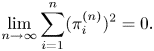 \begin{equation} {\lim_{n\rightarrow \infty}\sum_{i=1}^{n}(\pi_{i}^{(n)})^2=0}. \end{equation}
and from (A3) and (A4) it follows that
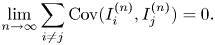 \begin{equation} {\lim_{n\rightarrow \infty}\sum_{i\neq j}{\rm Cov}(I_{i}^{(n)}, I_{j}^{(n)})=0}. \end{equation}
 Then, from (F1) and (F2) it follows that  ${\lim _{n\rightarrow \infty } d_{{\rm TV}}({L}(W_n), {\rm Poi}(\lambda _n))=0}$, and this completes the proof of Theorem 1.
Proof. (Assertion 1). If  $p=P(X_{ij})=0$ then $X_{ij}$ has Bernoulli distribution which is log-concave; or if $p\geq 1/3$ then $2X_{ij}$ has log-concave distribution (i.e., for integers $u\geq 1$, $(p(u))^2\geq p(u-1)p(u+1)$). Proposition 1 and Corollary 2 [Reference Ross6] hold in our model with $p=0$ or $p\in [1/3, 1)$, and therefore ${\sum _{i=1, i\neq j}^{n}I_{i}^{(n)}|I_{j}^{(n)}=1}$ is stochastically smaller than ${\sum _{i=1, i\neq j}^{n}I_{i}^{(n)}}$. Therefore, from the Corollary 2.C.2 [Reference Barbour, Holst and Janson1] we obtain (A1).
Proof. (Assertion 2). Follows from [Reference Feller4, pp. 552–553, Thms. 2 or 3].
Proof. (Assertion 3). Follows from Assertion 2 combined with [Reference Cramér3] result on p. 374 of his book.
Proof. (Assertion 4). Recall that  ${s_1=X_{12}+X_{13}+\cdots +X_{1n}}$ and ${ s_2=X_{21}+X_{23}+\cdots +X_{2n}}$. Hence, condition on the event ${X_{12}=k, k\in \{0, 1/2, 1\}}$, $s_1$ and $s_2$ are independent. Let ${s_{1{'}}=X_{13}+\cdots +X_{1n}, s_{2{'}}=X_{23}+\cdots +X_{2n}}$ and denote by ${s_{1{'}}^{*}, s_{2{'}}^{*}}$ the corresponding normalized scores (zero expectation and unit variance). We have,
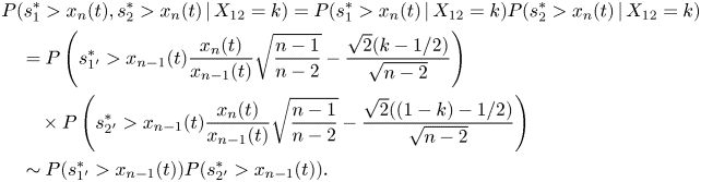 \begin{align} &P(s_{1}^{*}\gt x_n(t), s_{2}^{*}\gt x_n(t)\,|\,X_{12}=k )=P(s_{1}^{*}\gt x_n(t)\,|\,X_{12}=k ) P(s_{2}^{*}\gt x_n(t)\,|\,X_{12}=k )\nonumber\\ &\quad =P\left(s_{1{'}}^{*}\gt x_{n-1}(t)\frac{x_{n}(t)}{x_{n-1}(t)}\sqrt{\frac{n-1}{n-2}}-\frac{\sqrt{2}(k-1/2)}{\sqrt{n-2}}\right)\nonumber\\ &\qquad \times P\left(s_{2{'}}^{*}\gt x_{n-1}(t)\frac{x_{n}(t)}{x_{n-1}(t)}\sqrt{\frac{n-1}{n-2}}-\frac{\sqrt{2}((1-k)-1/2)}{\sqrt{n-2}} \right) \nonumber\\ &\quad \sim P(s_{1{'}}^{*}\gt x_{n-1}(t)) P(s_{2{'}}^{*}\gt x_{n-1}(t)). \end{align}
Combining (F3) with the formula of total probability we obtain
 \[ P(s_{1}^{*}\gt x_n(t), s_{2}^{*}\gt x_n(t))\sim P(s_{1{'}}^{*}\gt x_{n-1}(t)) P(s_{2{'}}^{*}\gt x_{n-1}(t)), \]
and combining it with Assertion 3 we obtain (A4).
Acknowledgement
I am grateful to Pavel Chigansky for pointing out my mistake.

