


1. Introduction
Non-diffusive transport occurs when there is a conserved quantity that can be rearranged in the system but not destroyed (Del-Castillo-Negrete Reference Del-Castillo-Negrete2010). One practical example is the transport of potential vorticity in the quasi-geostrophic model, which has a wide range of applications in oceanography and atmospheric science (Nigam & DeWeaver Reference Nigam and DeWeaver2015). When the horizontal scales are dominant, this system is analogously described by two-dimensional (2-D) incompressible Euler equations in the vorticity form, for which the conserved vertical component of the vorticity behaves as a passive scalar (Majda & Tabak Reference Majda and Tabak1996).
We ask a simple question: Given some highly complex two-dimensional distribution of a scalar field  $f_0(x,y)$, what is the simplest distribution $f_T(x,y)$ that can be obtained by transport with an arbitrary velocity field? We quantify ‘simplest’ by the desire to minimise gradients in $f_T$, so that we seek to minimise a measure like the Dirichlet seminorm, given by the surface integral
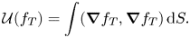 \begin{equation} \mathcal{U}(f_T)=\int (\boldsymbol{\nabla} f_T,\boldsymbol{\nabla} f_T) \,\text{d} S. \end{equation}
Arnold & Khesin (Reference Arnold and Khesin1998) investigated possible minimal states under  $\mathcal {U}(f_T)$, but for complex initial conditions $f_0$, the minimal state $f_T$ is not immediately known and must be computed numerically.
Perhaps surprisingly, our particular motivation comes from an attempt to understand the turbulent relaxation of 3-D magnetic fields in plasmas. In these 3-D resistive magnetohydrodynamic (MHD) simulations (Yeates, Hornig & Wilmot-Smith Reference Yeates, Hornig and Wilmot-Smith2010; Pontin et al. Reference Pontin, Wilmot-Smith, Hornig and Galsgaard2011, Reference Pontin, Candelaresi, Russell and Hornig2016), an initially braided magnetic field is allowed to evolve without a driving force until it reaches a quasi-steady state. The relaxed state is usually simple, and made of nearly uniformly twisted flux tubes. For example, the  $\mathcal {T}=2$ model from Yeates et al. (Reference Yeates, Hornig and Wilmot-Smith2010) is shown in figure 1(a–c). To appreciate the relevance of 2-D advection, note that the topological structure of braided magnetic fields may be completely characterised by a single invariant number attached to each magnetic field line. This is called the field line helicity (FLH) (Yeates & Hornig Reference Yeates and Hornig2013, Reference Yeates and Hornig2014), denoted by
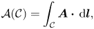 \begin{equation} \mathcal{A}(\mathcal{C})=\int_\mathcal{C} \boldsymbol{A}\boldsymbol{\cdot} \,\text{d} \boldsymbol{l}, \end{equation}
where  $\boldsymbol {A}(x,y,z,t)$ is a suitable vector potential for the magnetic field $\boldsymbol {B}=\boldsymbol {\nabla }\times \boldsymbol {A}$ and $\mathcal {C}$ is a magnetic field line (Russell et al. Reference Russell, Yeates, Hornig and Wilmot-Smith2015; Yeates & Page Reference Yeates and Page2018). The FLH has the physical interpretation of the net magnetic flux around the given field line (Yeates & Hornig Reference Yeates and Hornig2011), and in braided magnetic fields may be viewed as a 2-D scalar distribution on any cross-sectional surface. It is observed in these simulations that magnetic relaxation simplifies the cross-sectional FLH pattern as if it is being ‘unstirred’ by an effective flow $\boldsymbol {w}$; see figure 1(d–f) for the case of the $\mathcal {T}=2$ model.
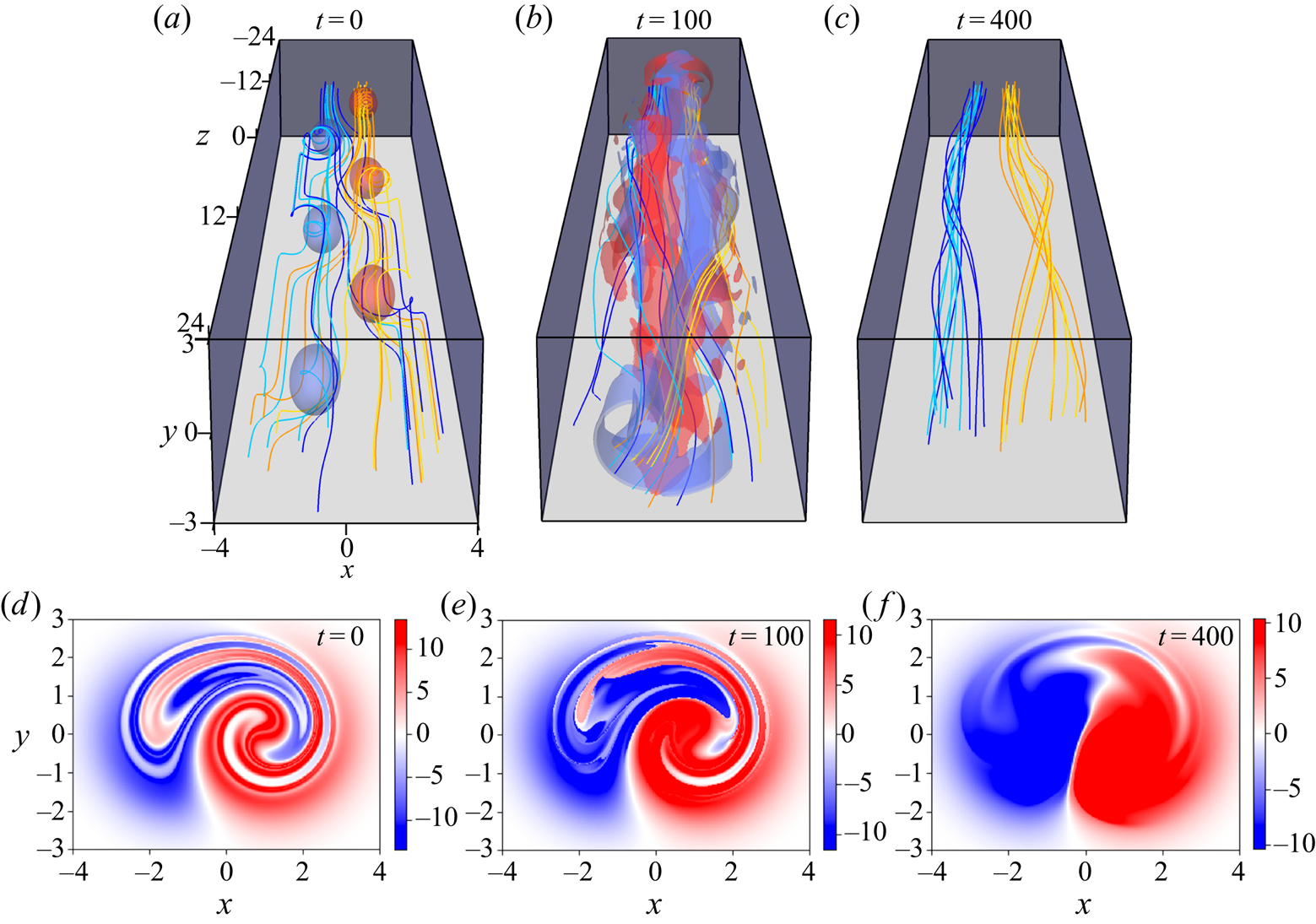
Figure 1. Magnetic reconnection of an initially braided magnetic field ( $\mathcal {T}=2$ model; for more details see Yeates et al. Reference Yeates, Hornig and Wilmot-Smith2010). (a–c) Blue and orange magnetic field lines are traced from distinct disks on the bottom plane at $z=-24$; these field lines are highly mixed at $t=0$, but magnetic reconnection separates them into a pair of separate oppositely twisted flux tubes. Red/blue volumes in (a,b) represent the iso-surfaces of the positive/negative current density. (d–f) The corresponding FLH on the boundary cross-section $z=24$. Time is measured in units of Alfvén time.
The evolution equation for the FLH, which was obtained by Russell et al. (Reference Russell, Yeates, Hornig and Wilmot-Smith2015), throws further light on the role of advection. First, note that the electric field  $\boldsymbol {E}$ can be decomposed into perpendicular and parallel components as $\boldsymbol {E} = -\boldsymbol {w}\times \boldsymbol {B} + \boldsymbol {\nabla } \psi$, where $\boldsymbol{w}$ is known as a field line velocity, $\psi (x,y,t)=\int _{\boldsymbol {x}_{-}}^{\boldsymbol {x}}\eta \,\boldsymbol {j}\boldsymbol {\cdot } \,\text {d} \boldsymbol {l}$ is a voltage that gives the parallel electric field, $\eta$ is the electrical resistivity and $\boldsymbol {j}=\boldsymbol {\nabla }\times \boldsymbol {B}$ is the current. From the analysis shown in Russell et al. (Reference Russell, Yeates, Hornig and Wilmot-Smith2015) (see also Yeates Reference Yeates2020), the evolution equation of the FLH is then
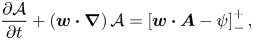 \begin{equation} \frac{\partial \mathcal{A}}{\partial t}+ \left(\boldsymbol{w} \boldsymbol{\cdot}\boldsymbol{\nabla}\right)\mathcal{A} = \left[\boldsymbol{w}\boldsymbol{\cdot} \boldsymbol{A} -\psi\right]^{+}_{-}, \end{equation}
where the superscript  $+$ and subscript $-$ signify evaluation at the points where the field line exits and enters the domain (cf. (12) in Russell et al. Reference Russell, Yeates, Hornig and Wilmot-Smith2015). In practice, $\psi$ can be chosen so that the terms on the right-hand side are non-zero only at one boundary, and if the FLH is inspected on that boundary, then (1.3) reduces to a 2-D problem governing $\mathcal {A}(x,y,t)$. The left-hand side of (1.3) signifies advection of the FLH with the field line flow $\boldsymbol {w}$ (generally distinct from the plasma motion), which mathematically establishes the relevance of advection to this problem. Advection is not the only relevant process, due to (non-diffusive) terms on the right-hand side of (1.3). However, Russell et al. (Reference Russell, Yeates, Hornig and Wilmot-Smith2015) showed that the $\psi$ terms are relatively small in complex magnetic fields, and that the $\boldsymbol {w}\boldsymbol {\cdot } \boldsymbol {A}$ terms integrate to (nearly) zero over myriad small regions containing opposite polarity (paired increases and decreases of $\boldsymbol {w}\boldsymbol {\cdot }\boldsymbol {A}$). This leaves the advection term as the only non-negligible term of a fundamentally global nature, consistent with the intuition drawn from simulations that 2-D advection is the process from which to begin understanding the observed simplification of the FLH during 3-D turbulent magnetic relaxation. It is therefore of interest to determine the simplest contour pattern of $\mathcal {A}$ consistent with a given initial distribution, so as to test whether passive advection is playing a controlling role in the turbulent relaxation, and help identify any significant effects attributable to the other terms in (1.3).
The actual computation to search for the minimal ‘unstirred’ state is independent of the motivating magnetic braid problem, and has more in common with the well-studied problem of transport and mixing of passive tracers in engineering (Warhaft Reference Warhaft2000). Usually the objective is to find a velocity field that mixes  $f_0$ as efficiently as possible and maximises $\mathcal {U}(f_T)$, but the inverse problem is essentially analogous owing to the reversibility of the advection equation. To better quantify the homogenisation of the passive tracer, several other norms have also been used in the literature, including a class of ‘mix-norms’ (Mathew, Mezić & Petzold Reference Mathew, Mezić and Petzold2005; Thiffeault Reference Thiffeault2012). This type of norm has recently been applied to the optimisation problems of mixing in 2-D plane Poiseuille flow (Foures, Caulfield & Schmid Reference Foures, Caulfield and Schmid2014) and stratified plane Poiseuille flow (Marcotte & Caulfield Reference Marcotte and Caulfield2018) using variational methods. From this perspective, our unstirring problem may be considered as an interesting test of the state-of-the-art of the methods used in this branch of fluid dynamics.
In this paper, the constraint that the final state must be reachable by passive advection makes the minimisation a non-trivial computational task. We consider two approaches to identify suitable unstirring velocity fields  $\boldsymbol {u}$. One is a variational approach where we test both the Dirichlet seminorm and a mix-norm as measures of the homogenisation. Inspiration for how to implement the constraint of passive advection comes from work with adjoint-based methods both in pipe flow (identifying the seed to chaos; Kerswell, Pringle & Willis Reference Kerswell, Pringle and Willis2014) and in kinematic dynamo theory (finding the magnetic instability; Willis Reference Willis2012). The variational approach allows in principle for any possible (incompressible) velocity field, although we might expect that the obtained velocity field will in practice be constrained by the structure of $f_0$ in some way. Studies of mixing have found that the topological structure of the final, mixed, state can be related directly to the properties of the velocity field that produced it. For example, in Ottino (Reference Ottino1990), the islands or holes among chaotic fluid regions are linked to periodic points created by a sequence of stirring motions.
The second approach to unstirring that we consider is rather different, in that the velocity field is prescribed in a pre-defined way based on the pattern of  $f$. It is chosen to guarantee simplification of the pattern at any instant, using the magnetic relaxation method (Moffatt Reference Moffatt1990; Linardatos Reference Linardatos1993; Moffatt & Dormy Reference Moffatt and Dormy2019). This works because the magnetic field lines in a 2-D ideal-MHD flow are material lines. These field lines are contours of a scalar flux function, which is analogous to the scalar field $f$ in our unstirring problem, and a corresponding MHD solution is used for the velocity field $\boldsymbol {u}$. Thus it is no longer a variational calculation but a single well-defined evolution from $f_0$ to $f_T$, during which the Dirichlet seminorm – which is analogous to the magnetic energy – is minimised. The resulting patterns of $f_T$ have been studied by Linardatos (Reference Linardatos1993) for simple $f_0$ distributions with either a single maximum or a pair of local maxima with a saddle point between. The system minimises the length of the contours while preserving the area enclosed, making them circular where this is not prevented by other considerations such as the domain boundary. An interesting feature is that the saddle point collapses to a thin current sheet in the relaxed state, and Moffatt & Dormy (Reference Moffatt and Dormy2019) conjecture that every saddle point in $f_0$ will collapse to a finite-length current sheet in $f_T$ (see also Arnold & Khesin Reference Arnold and Khesin1998). This suggests what kind of patterns might be expected in the unstirred state.
The remainder of this paper is organised as follows. We define the problem in § 2, including the equations solved in both the variational (§ 2.1) and the magnetic relaxation (§ 2.2) approaches. The numerical methods are described in § 2.3, before comparing them for simple test cases in § 2.4. In § 3, we present the results for more complex initial distributions using the magnetic relaxation method. A summary and discussion of the results are presented in § 4.
2. Problem set-up and methods
Given a density function  $f(x,y,t)$ in a domain $D\in \mathbb {R}^2$, with initial distribution $f(x,y,0)=f_0(x,y)$, we define a time-dependent energy by the Dirichlet seminorm of $f$,
$f$,
 \begin{equation} E(t) = \langle |\boldsymbol{\nabla} f|^2\rangle, \end{equation}
where  $\langle \cdots \rangle = \iint _D \cdots \,\text {d} S$ is the surface integral over $D$. For the final state $f_T=f(x,y,T)$, this energy is (1.1). We search for the minimum-energy state $f_T$ reachable under the advection equation,
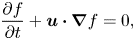 \begin{equation} \frac{\partial f}{\partial t }+\boldsymbol{u}\boldsymbol{\cdot} \boldsymbol{\nabla} f =0, \end{equation}
in a fixed time interval  $[0,T]$. The velocity field is constrained to be incompressible,
 \begin{equation} \boldsymbol{\nabla}\boldsymbol{\cdot}\boldsymbol{u}=0, \end{equation}
so that the area inside any closed material curve is conserved. We assume  $f$ obeys periodic boundary conditions or $\boldsymbol {\nabla } f|_{\partial D}= 0$. Having formally defined the problem in this way, we can derive structural constraints on the final state, $f_T$. For example, consider a small deformation which under (2.2) and (2.3) takes the form $\delta f=-\boldsymbol {\xi }\boldsymbol {\cdot }\boldsymbol {\nabla } f$ where $\boldsymbol {\xi }=\boldsymbol {\nabla }\times \zeta (x,y)\hat {\boldsymbol {z}}=\boldsymbol {\nabla }\zeta (x,y)\times \hat {\boldsymbol {z}}$ and $\boldsymbol {\xi }\boldsymbol {\cdot }\boldsymbol {n}|_{\partial D}=0$. Using either type of boundary condition mentioned above,
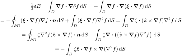 \begin{gather} \tfrac{1}{2}\delta E=\int_D \boldsymbol{\nabla} f \boldsymbol{\cdot} \boldsymbol{\nabla} \delta f \,\text{d} S={-}\int_D \boldsymbol{\nabla} f \boldsymbol{\cdot} \boldsymbol{\nabla} (\boldsymbol{\xi}\boldsymbol{\cdot} \boldsymbol{\nabla} f)\,\text{d} S\nonumber\\ ={-}\oint_{\partial D} (\boldsymbol{\xi}\boldsymbol{\cdot} \boldsymbol{\nabla} f)\boldsymbol{\nabla} f\boldsymbol{\cdot} \boldsymbol{n}\,\text{d} S+\int_D(\boldsymbol{\xi}\boldsymbol{\cdot} \boldsymbol{\nabla} f)\nabla^2 f\,\text{d} S =\int_D\boldsymbol{\nabla} \zeta \boldsymbol{\cdot}(\hat{\boldsymbol{z}}\times \boldsymbol{\nabla} f)\nabla^2 f \,\text{d} S\nonumber\\ =\oint_{\partial D} \zeta \nabla^2 f (\hat{\boldsymbol{z}}\times \boldsymbol{\nabla} f)\boldsymbol{\cdot} \boldsymbol{n}\,\text{d} S- \int_D\zeta\boldsymbol{\nabla}\boldsymbol{\cdot} \left((\hat{\boldsymbol{z}}\times \boldsymbol{\nabla} f)\nabla^2 f\right)\,\text{d} S\nonumber\\ ={-}\int_D\zeta \hat{\boldsymbol{z}}\boldsymbol{\cdot} \boldsymbol{\nabla} f \times\boldsymbol{\nabla}(\nabla^2 f)\,\text{d} S. \end{gather}
A state  $f_T$ that minimises $E(t)$ under (2.2) and (2.3) must therefore satisfy
 \begin{equation} \boldsymbol{\nabla} f_T \times\boldsymbol{\nabla}\left(\nabla^2 f_T\right) = 0, \end{equation}
so that  $\nabla ^2f_T$ is constant along the contours of $f_T$. In addition, the structure of $f_T$ is related to that of $f_0$ because the evolution preserves the topology of the contours of $f$. Specifically, for $f(x,y)=f_c$ (where $f_c\neq 0$), the enclosed area is invariant, which we can represent with a signature function (Moffatt Reference Moffatt1990; Arnold & Khesin Reference Arnold and Khesin1998),
 \begin{equation} \mathcal{S}(f_c) = \begin{cases} \displaystyle\iint_{f(x,y)\geq\, f_c} \,\text{d} S & \textrm{if}\ f_c > 0,\\ \displaystyle\iint_{f(x,y)\leq\, f_c} \,\text{d} S & { \rm if}\ f_c < 0. \end{cases} \end{equation}
 We now give two complementary approaches to finding a suitable  $\boldsymbol {u}$: (i) the variational method imposes fewer restrictions on $\boldsymbol {u}$ but has no guarantee of convergence; (ii) the magnetic relaxation method uses a specific MHD solution for $\boldsymbol {u}$ to guarantee monotonically decreasing $E(t)$, as we will show in § 2.2. It turns out that both methods can find the expected minimal energy state of $f_T$ for simple initial states $f_0$, but for complicated cases only the second method is numerically stable. We will describe each method in more detail below.
2.1. Variational method
Given the initial distribution  $f_0=f(x,y,0)$ of a passive scalar field $f$, the variational method searches for the optimal velocity field $\boldsymbol {u}$ with respect to an augmented Lagrangian $\mathcal {L}$. In fluid mixing and transport studies, the Lagrangian is commonly defined by a measure of homogenisation and other constraints, such as the Navier–Stokes equation and the normalisation condition of a seed perturbation field. Although it would be intuitive to use the Dirichlet seminorm to quantify homogenisation, a ‘mix-norm’ $\langle |\nabla ^{-1}f_T|^2\rangle$ has been shown to be numerically robust and efficient (Thiffeault Reference Thiffeault2012; Marcotte & Caulfield Reference Marcotte and Caulfield2018). We therefore define a generic Lagrangian applicable to two measures of homogenisation as
 \begin{equation} {\mathcal{L}} = \langle |\nabla^{\theta} f_T|^2\rangle +\theta \langle \varPi\boldsymbol{\nabla}\boldsymbol{\cdot}{\boldsymbol{u}}\rangle + \theta \int_0^T\left\langle \varGamma\left(\frac{\partial f}{\partial t} +\boldsymbol{u}\boldsymbol{\cdot}\boldsymbol{\nabla} f \right)\right\rangle \,\text{d} t, \end{equation}
where  $\theta =1$ represents the Dirichlet seminorm and $\theta =-1$ represents a mix-norm, and $f_T=f(x,y,T)$ is the final unstirred state. When $f$ becomes less mixed, the Dirichlet seminorm goes down while this mix-norm goes up. Thus, we minimise the Lagrangian when $\theta =1$, and maximise the Lagrangian when $\theta =-1$. Meanwhile, $\varGamma (x,y,t)$ and $\varPi (x,y)$ are Lagrange multipliers which impose constraints (2.2) and (2.3) respectively, and $\boldsymbol {u}(x, y)$ is a time-independent velocity field. We can also formulate (2.7) with a general time-dependent field $\boldsymbol {\tilde {u}}(x,y,t)$, in which case we also need a time-dependent Lagrange multiplier $\tilde {\varPi }(x,y,t)$. With time-dependent $\boldsymbol {\tilde {u}}$, we found the numerical error tends to accumulate at each time step, so in this paper we present the variational method results only with a steady velocity field. Unlike similar models where the flow scale $u^*$ carries important physical meaning (Pringle, Willis & Kerswell Reference Pringle, Willis and Kerswell2012; Chen, Herreman & Jackson Reference Chen, Herreman and Jackson2015), in our case, the velocity field can always be rescaled with arbitrary time and length scales as $u^*\sim L^*/t^*$, while still giving the same final state of $f$. Since we are mostly interested in the spatial distribution of $\boldsymbol {u}$, there is then no need to impose the normalisation of $\boldsymbol {u}$ as a separate constraint in (2.7).
Each of the variational derivatives of  ${\mathcal {L}}$ has to vanish separately for the optimal solution, since
 \begin{equation} \delta{\mathcal{L}} = \left\langle\frac{\delta{\mathcal{L}}}{\delta f_T}\delta f_T\right\rangle+ \left\langle\frac{\delta{\mathcal{L}}}{\delta{{\varPi}}}\delta{{\varPi}}\right\rangle+\left\langle\frac{\delta{\mathcal{L}}}{\delta\boldsymbol{u}}\boldsymbol{\cdot}\delta\boldsymbol{u}\right\rangle +\int_0^T\left\langle \delta\varGamma\frac{\delta{\mathcal{L}}}{\delta{{\varGamma}}}\right\rangle\,\text{d} t + \int_0^T\left\langle \delta f\frac{ \delta{\mathcal{L}}}{\delta f}\right\rangle \,\text{d} t. \end{equation}
These variational derivatives are derived explicitly in appendix A. Note that, in (2.8), we have already taken into account that the boundary terms vanish when  $\boldsymbol {u}$ and $f$ either both satisfy periodic boundary conditions or satisfy $\boldsymbol {u}\boldsymbol {\cdot }\boldsymbol {n}=0$ and $\boldsymbol {\nabla } f|_{\partial D}=0$ respectively. By setting all variational derivatives to zero except that of the unknown optimal velocity field $\boldsymbol {u}$, we obtain a coupled system of Euler–Lagrange equations. We solve these iteratively by adapting the adjoint method (see the review by Luchini & Bottaro (Reference Luchini and Bottaro2014)), which has typically been applied to the full Navier–Stokes equations rather than the advection equation alone. Specifically, we iterate the following four steps until the variational derivative $\delta {\mathcal {L}}/\delta \boldsymbol {u}$ also converges to zero:
(i) Calculate $f$ forward in time from $t=0$ to $t=T$ using the advection equation (2.2), which is equivalent to solving $\delta {\mathcal {L}}/\delta \varGamma =0$ for $t: 0\rightarrow T$.
(ii) Apply the terminal condition
$\delta {\mathcal {L}}/\delta f_T=0$, so that
(2.9)where the usual Laplacian operator corresponds to\begin{equation} \varGamma_T =2\theta\nabla^{2\theta} f_T, \end{equation}$\theta =1$ (minimising the Dirichlet seminorm), and the inverse Laplacian operator corresponds to $\theta =-1$ (maximising one type of mix-norm).(iii) Calculate
$\varGamma$ backward in time from $t=T$ to $t=0$ using the adjoint advection equation
(2.10)which is equivalent to enforcing\begin{equation} \frac{\partial \varGamma}{\partial t} +\boldsymbol{u}\boldsymbol{\cdot}\boldsymbol{\nabla} \varGamma=0, \end{equation}$\delta {\mathcal {L}}/\delta f=0$ with the incompressible condition (2.3) for $t: T\rightarrow 0$.(iv) Finally, the update scheme for
$\boldsymbol {u}$ is
(2.11)where\begin{equation} \boldsymbol{u}:=\boldsymbol{u}-\theta\varDelta_u\frac{\delta{\mathcal{L}}}{\delta\boldsymbol{u}}, \end{equation}$\varDelta _u> 0$ is a step size that we adjust and the gradient is given by
(2.12)This method will in principle reach a local minimum with consecutive steps; however, the convergence is not guaranteed should the search algorithm (iv) become trapped or encounter numerical instabilities.\begin{equation} \frac{\delta{\mathcal{L}}}{\delta\boldsymbol{u}} = \theta\left(-\boldsymbol{\nabla}\varPi +\int_0^T\varGamma\left(\boldsymbol{\nabla} f \right)\,\textrm{d}t\right). \end{equation}


Section 2.3.1 provides numerical details of both cases ( $\theta = {\pm }1$), while convergence of all methods is compared in § 2.4.
2.2. Magnetic relaxation method
The magnetic relaxation method relates the reduction of the Dirichlet seminorm  $E(t)$ to the relaxation process of a 2-D magnetic field in ideal MHD (see § 1 for the background information). To achieve this, we define a fictitious magnetic field $\boldsymbol {B}(x,y,t)$ on $D$ whose field lines at any time are the contours of the function $f$, given by
 \begin{equation} \boldsymbol{B}=\boldsymbol{\nabla}\times f (x,y,t)\hat{\boldsymbol{z}}. \end{equation}
The energy of this magnetic field is proportional to our energy measure (2.1), since
 \begin{equation} \langle B^2\rangle = \langle |\boldsymbol{\nabla} f|^2\rangle = E(t). \end{equation}
Any momentum equation that lowers the magnetic energy ideally, i.e. preserving the isocontours of  $f$, can therefore be used to reduce $E(t)$. We choose to use a magnetic relaxation scheme of the form
 \begin{equation} \mu\nabla^2\boldsymbol{u}+(\boldsymbol{\nabla}\times\boldsymbol{B})\times \boldsymbol{B}-\boldsymbol{\nabla} P=0, \end{equation}
which describes the balance of fluid viscosity, Lorentz force and pressure. The first term in (2.15) represents viscous dissipation where  $\mu$ is an artificial viscosity; the second term represents the Lorentz force by taking the current as $\boldsymbol{j}=\boldsymbol {\nabla }\times \boldsymbol {B}$. We include the pressure $P(x,y,t)$ here so that $\boldsymbol {u}(x,y,t)$ may be chosen to satisfy the incompressibility condition (2.3). Using a viscous term rather than a frictional term $\mu \boldsymbol {u}$ (like, for example, Linardatos Reference Linardatos1993) avoids some limitations of the frictional approach such as the inability of $\boldsymbol {B}=0$ points to move (Low Reference Low2013). We also set $\mu =1$ so that the typical evolution time is of the order $t^*\sim (l^*/f^*)^{2}$, which is estimated by substituting (2.13) into (2.15). As the homogenisation of $f$ increases, the length scale $l^*$ increases so the relaxation is expected to slow down proportionally. If we rewrite the Lorentz force term in (2.15) as
 \begin{equation} (\boldsymbol{\nabla}\times\boldsymbol{B})\times \boldsymbol{B}={-}\nabla^2f \hat{\boldsymbol{z}}\times(\boldsymbol{\nabla} f\times \hat{\boldsymbol{z}})={-}\nabla^2 f(\boldsymbol{\nabla} f), \end{equation}
we see clearly that both  $\nabla ^2f$ and the gradient $\boldsymbol {\nabla } f$ (including its magnitude and direction) play a role in determining the velocity field $\boldsymbol {u}$. By writing
 \begin{equation} \boldsymbol{u}=\boldsymbol{\nabla}\times \psi (x,y,t)\hat{\boldsymbol{z}} \end{equation}
and taking the curl of (2.15), we can calculate  $\boldsymbol {u}$ at a given time by solving the biharmonic equation
 \begin{equation} \mu\nabla^4\psi=\hat{\boldsymbol{z}}\boldsymbol{\cdot} \boldsymbol{\nabla} f\times\boldsymbol{\nabla}(\nabla^2 f). \end{equation}
For this approach, we either assume periodic boundary conditions for  $\psi$ or set
 \begin{equation} \psi|_{\partial D}=\nabla^2\psi|_{\partial D}=0, \end{equation}
which implies the velocity field satisfies not quite the no-slip condition but rather
 \begin{equation} \boldsymbol{u}\boldsymbol{\cdot} \boldsymbol{n}|_{\partial D} =0, \quad \boldsymbol{\nabla}\times\boldsymbol{u}|_{\partial D} =0. \end{equation}
Combining (2.2), (2.15), (2.16) and (2.20a,b), we find
 \begin{gather} \frac{1}{2}\frac{\partial E(t)}{\partial t}= \int_D \boldsymbol{\nabla} f \boldsymbol{\cdot}\frac{\partial (\boldsymbol{\nabla} f)}{\partial t}\,\text{d} S ={-}\int_D\nabla^2 f \frac{\partial f}{\partial t}\,\text{d} S +\oint_{\partial D} \frac{\partial f}{\partial t} (\boldsymbol{\nabla} f \boldsymbol{\cdot}\boldsymbol{n})\,\text{d} l\nonumber\\ =\int_D \nabla^2 f (\boldsymbol{u}\boldsymbol{\cdot}\boldsymbol{\nabla} f)\,\text{d} S =\int_D \boldsymbol{u}\boldsymbol{\cdot}(\mu \nabla^2 \boldsymbol{u})\,\text{d} S - \int_D \boldsymbol{u}\boldsymbol{\cdot} \boldsymbol{\nabla} P\,\text{d} S\nonumber\\ ={-}\mu\int_D|\boldsymbol{\nabla}\times\boldsymbol{u}|^2 \,\text{d} S + \oint_{\partial D} \boldsymbol{u}\boldsymbol{\cdot} [(\boldsymbol{\nabla}\times\boldsymbol{u})\times \boldsymbol{n}] \,\text{d} l-\oint_{\partial D} P (\boldsymbol{u} \boldsymbol{\cdot}\boldsymbol{n})\,\text{d} l \nonumber\\ ={-}\mu\int_D|\boldsymbol{\nabla}\times\boldsymbol{u}|^2 \,\text{d} S \leq 0. \end{gather}
This shows that the Dirichlet seminorm  $E(t)$ will decrease monotonically, in direct proportion to the enstrophy
 \begin{equation} \varepsilon(t)=\langle|\boldsymbol{\nabla}\times \boldsymbol{u}|^2\rangle. \end{equation}
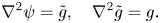
If it converges then the final minimal energy state will obey  $\boldsymbol {\nabla }\times \boldsymbol {u}=0$. Since this corresponds to $\nabla ^2\psi \equiv 0$, (2.18) shows that such a state $f_T$ must satisfy
 \begin{equation} \boldsymbol{\nabla} f_T\times\boldsymbol{\nabla}(\nabla^2f_T)= 0, \end{equation}
which is consistent with (2.5). A similar derivation that shows (2.23) but with the frictional term in place of the viscous term is discussed in Moffatt & Dormy (Reference Moffatt and Dormy2019). Note that the boundary conditions (2.19) also imply that  $\boldsymbol {u}=0$ for such a state; alternatively, periodic boundaries would allow for a uniform velocity.
2.3. Numerical schemes
In this section we discuss the numerical implementation of the two methods mentioned above.
2.3.1. Variational method
As described in § 2.1, we iterate four steps to search for the optimal velocity field  $\boldsymbol {u}$: (i) compute forward advection for $f$, (ii) apply the terminal condition, (iii) compute backward (adjoint) advection for $\varGamma$ and (iv) update $\boldsymbol {u}$. Steps (i) and (iii) are discretised in space using a pseudo-spectral method, which is also used to evaluate the derivative in the terminal condition (ii). We also tested with a finite difference method to solve the advection equation, but the accuracy of the unstirred state $f_T$ was not sufficient for this iterative process, i.e. any small deviation in $f_T$ will feed back into the update step (iv). The time discretisation uses a fourth-order Runge–Kutta method, with adaptive time step chosen as
 \begin{equation} \Delta t=\frac{a_s \,d}{\max \{ |\boldsymbol{u}_{i,j}|\}}, \end{equation}
where  $a_s=0.1$ is a safety factor, $d=\Delta x=\Delta y$ is the grid spacing and $\boldsymbol {u}_{i,j}$ are the values of $\boldsymbol {u}$ at the grid points.
To compute the variational derivative  $\delta \mathcal {L}/\delta \boldsymbol {u}$ in step (iv) as given by (2.12), we first compute $\boldsymbol {h}=\int _0^T(\boldsymbol {\nabla } f) \,\varGamma \,\text {d} t$ using the trapezium rule and then use this to find $\varPi$ (and hence $\boldsymbol {\nabla }\varPi$) by solving the Poisson problem
 \begin{equation} \nabla^2\varPi=\boldsymbol{\nabla} \boldsymbol{\cdot} \boldsymbol{h}, \end{equation}
using a Fourier finite difference method since the pseudo-spectral method is sensitive to numerical noise. We then use the Barzilai–Borwein method to update  $\boldsymbol {u}$. The step size in (2.11) is set to
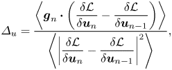 \begin{equation} \varDelta_u=\frac{\left\langle\boldsymbol{g}_n\boldsymbol{\cdot}\left(\dfrac{\delta{\mathcal{L}}}{\delta{{\boldsymbol{u}}_n}}-\dfrac{\delta{\mathcal{L}}}{\delta {{\boldsymbol{u}}_{n-1}} } \right)\right\rangle}{\left\langle \left|\dfrac{\delta{\mathcal{L}}}{\delta {{\boldsymbol{u}}_n} }-\dfrac{\delta{\mathcal{L}}}{\delta{{\boldsymbol{u}}_{n-1}} }\right|^2\right\rangle}, \end{equation}
where  $\boldsymbol {g}_n$ denotes the update $\boldsymbol {u}_{n+1}=\boldsymbol {u}_{n}+\boldsymbol {g}_n$ for $n>2$, computed from (2.12). We apply the standard 2/3 rule for de-aliasing when calulcating $\boldsymbol {u}$. The initial velocity is $\boldsymbol {u}=0$. The first two iterations have fixed $\varDelta _u=10^{-3}$. The time step $\Delta t$ is halved (effectively $a_s:=0.5a_s$) when the energy increases $E_n(T)> E_{n-1}(T)$ to reduce numerical errors. We stop the iteration when $\langle g^2\rangle <10^{-6}$.
2.3.2. Magnetic relaxation method
To implement this method, we discretise the advection equation (2.2) in time with the velocity  $\boldsymbol {u}$ at each time step derived from $f$ by solving the biharmonic equation (2.18) for the streamfunction $\psi$ in (2.17).
The advection equation is solved using LeVeque's scheme as described in Durran (Reference Durran2010) with the Van Leer flux limiter. This method limits the gradient of neighbouring grid points to computationally realistic values, so it is particularly suitable for dealing with complex patterns in  $f$. The time step is adaptive as in (2.24). To solve the biharmonic equation, we first use a second-order finite difference method to calculate the right-hand side, denoted by $g$. Next we solve two Poisson problems to get the solution for $\psi$ using a Fourier finite difference method,
 \begin{equation} \nabla^2 \psi=\tilde{g}, \quad \nabla^2\tilde{g}=g. \end{equation}
The algorithm that calculates  $\psi$ uses either Fourier transforms with periodic boundary conditions, or sine transforms for the boundary condition (2.19). The velocity field $\boldsymbol {u}$ is calculated from $\psi$ using a fourth-order finite difference method. Then we solve the advection equation for the next time step. We compute $E(t)$ at each time step to monitor the homogenisation of $f$. We stop the computation if $E(t)$ is found to increase.
2.4. Test cases
To facilitate the discussion of the two different approaches, from now on we will refer to the variational method as VM and the magnetic relaxation method as MR. In this section we compare the performance of the methods for simple test examples, which have periodic boundary conditions.
Our tests consider how well the methods unstir a sheared pattern towards a known minimal energy state. We create an initial state
 \begin{equation} f_0=\sin[{\rm \pi}(2x - \alpha\cos(k_y{\rm \pi} y))]\sin({\rm \pi} y), \end{equation}
where  $k_y$ is the wavenumber of the shearing and $\alpha$ is a parameter controlling the amount of shearing. The expected minimal energy state is
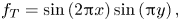 \begin{equation} f_T= \sin\left(2{\rm \pi} x\right)\sin\left({\rm \pi} y\right), \end{equation}
with energy  $E(T)=5{\rm \pi} ^2$, which would be reached by advection with a steady velocity field
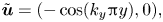 \begin{equation} \tilde{\boldsymbol{u}}=(- \cos(k_y{\rm \pi} y), 0), \end{equation}
precisely at time  $\alpha =T$. For MR, $T$ is determined by the evolution. In the examples presented, we choose $k_y=7$ so as to create non-trivial patterns. We then vary the value of $\alpha$ to see if the algorithms can still identify $\boldsymbol {u}$ when $f_0$ contains sharper gradients. Figure 2 shows the three initial conditions tested with increasing complexity from left to right. For VM in particular, we also test the two formulations which use either the Dirichlet seminorm ( $\theta =1$) or a mix-norm ( $\theta =-1$).

Figure 2. Initial conditions  $f_0$ with increasing complexity from (a) to (c), where $\alpha$ is the initial shearing strength.
The results for VM ( $\theta =\pm 1$) and MR are shown in table 1. For the simplest $f_0$ with $\alpha =0.1$, VM ( $\theta =1$) is not numerically stable: it does not converge with increased resolution $N$. In contrast, both VM ( $\theta =-1$) and MR are able to reach the expected minimal energy with the correct final state. In figure 3, we plot a few snapshots to show how $f_T$ evolves iteratively with VM ( $\theta =-1$) and how $f_0$ has been unstirred with MR. For VM ( $\theta =-1$), the shape of the recovered velocity field – as shown in figure 4 – is quite close to the expected solution, but differs in that (i) it picks up some $y$ component, and (ii) $u_x$ is not evolving much with each iteration in places where $f$ is zero (e.g. along the line $y=0$). These differences do not change the energy substantially, and indeed multiple velocity fields can reach the same $f_T$ pattern, e.g. two velocity fields that differ in their component along the $f$ contours will have the same $\boldsymbol {u}\boldsymbol {\cdot }\boldsymbol {\nabla } f$.

Figure 3. Selected snapshots during unstirring. Test run with  $N=512$ and $\alpha =0.1$. (a,c,e) VM ( $\theta =-1$). (b,d,f) MR. Both exhibit a reduction in shearing.
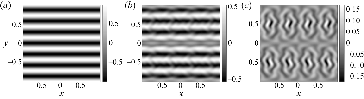
Figure 4. Comparison between obtained velocity field  $\boldsymbol {u}$ using VM ( $\theta =-1$) and the expected velocity field $\tilde {\boldsymbol {u}}$. Test run with $N=512$ and $\alpha =0.1$. (a) The expected $x$-component of the velocity field ${\tilde {u}_x}=- \cos (7{\rm \pi} y)$ (the expected $y$-component is ${\tilde {u}_y}=0$). (b) Pseudo-colour plot of ${u_x}$. (c) Pseudo-colour plot of ${u_y}$.
Table 1. Test results:  $T$ is the total time for advection; $\Delta E(T)$ is the difference between the obtained $E(T)$ and the expected minimal energy $5{\rm \pi} ^2\approx 49.348$.
 $^{a}$Best value achieved without meeting the convergence criterion.
In terms of performance, for  $\alpha =0.1$, VM ( $\theta =-1$) finds a slightly more accurate $f_T$ than MR, but the error is also more localised; see figure 5. The largest error of $f_T$ occurs where the expected value ${\tilde {f}_T}\approx 0$. VM is unable to prevent these discontinuities from forming. This proves to be problematic when the initial distribution contains sharper gradients, because the pseudo-spectral method that was needed for accuracy is unable to resolve the corresponding variational derivative $\delta \mathcal {L}/\delta \boldsymbol {u}$ for the update. For $\alpha \geq 0.3$, VM ( $\theta =-1$) struggles to converge while MR finds a minimal energy that is close ( $<2\,\%$) to the expected value. Note that for $\alpha =0.3$ case, even though the test run with VM ( $\theta =-1$) has met the convergence criterion, the number of time steps taken is huge and the minimal energy is not as low as we expect. In addition, with VM the optimisation may go in the wrong direction before it eventually converges, whereas with MR the convergence is gradual and smooth in terms of the change in $E(t)$ – see figure 6 for comparison. The MR method remains numerically stable for all $\alpha$.
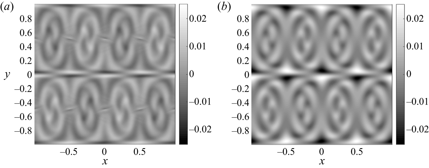
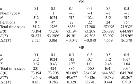
Figure 5. The difference between  $f_T$ and the expected solution ${\tilde {f}_T}=\sin (2{\rm \pi} x)\sin ({\rm \pi} y)$. Test run with $N=512$ and $\alpha =0.1$. (a) VM ( $\theta =-1$); the actual maximal magnitude of error for VM is $0.014$. (b) MR, where the maximum magnitude is $0.025$.
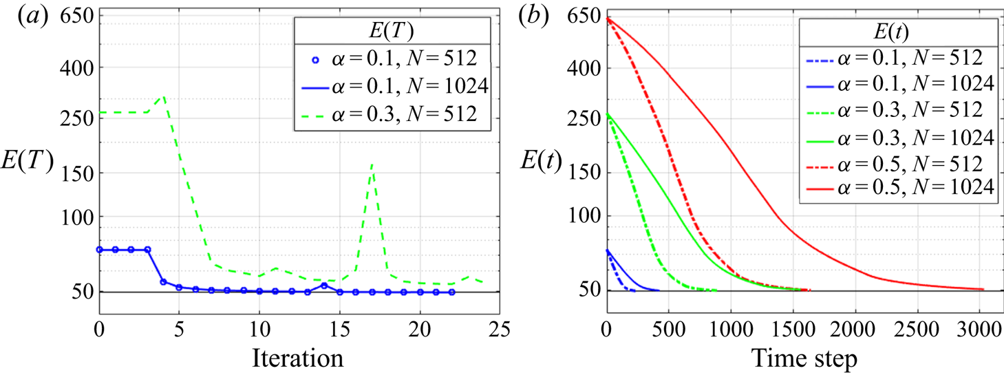
Figure 6. Comparison of convergence. (a) VM ( $\theta =-1$), showing $E(T)$ as a function of the iteration number. For $\alpha =0.1$ the results with $N=512, 1024$ coincide, and for $\alpha =0.5$ the lowest $E(T)$ did not meet the convergence criterion and hence is excluded from this plot. (b) MR, showing $E(t)$ as a function of time step during the relaxation.
Based on the test runs, we find these two approaches each have their own benefits and limitations for finding the optimal  $f_T$. On the one hand, VM ( $\theta =-1$) gives a more accurate result for simple initial conditions, but the lack of diffusion or any additional ‘smoothing’ constraint in the Lagrangian means little control over the sharpness of the gradient $\boldsymbol {\nabla } f$ in regions where the expected value ${\tilde {f}_T}\approx 0$. On the other hand, MR has restricted the form of the velocity field so the search for the minimal energy state is not necessarily optimal, but the obtained unstirred state $f_T$ appears to be smoother for simple initial conditions, as seen in figure 5; also it is the most robust method for general initial conditions. Therefore, we move on to analyse complex patterns using only MR.
3. Results for complex patterns
Our original motivation for this study was to determine the unstirred pattern of a passive scalar field, namely the FLH, extracted on 2-D cross-sections of 3-D simulations. For this purpose, we consider two initial FLH patterns from the  $\mathcal {T}=2$ case and $\mathcal {T}=3$ case studied by Yeates et al. (Reference Yeates, Hornig and Wilmot-Smith2010). The number $\mathcal {T}$ refers to the topological degree of the underlying (3-D) field line mapping, which is preserved in the 3-D simulation and controls the number of large-scale regions of the FLH in the relaxed state (see also Yeates, Russell & Hornig Reference Yeates, Russell and Hornig2015) – effectively the number of large-scale magnetic flux tubes in the relaxed state. Specific details of the construction are given in appendix B. We show contour plots of the initial states $f_0$ in the top row of figure 7. These initial patterns are much more complicated than our test cases in § 2.4. Due to regions with negative and positive values being in close proximity to one another, they are numerically challenging to unstir since the gradient of $f$ can be large. The computational domain $D: [-20, 20]\times [-20, 20]$ is chosen to be large enough so that $\boldsymbol {\nabla } f\approx 0$ at the boundary. The grid resolution is $6000\times 6000$.
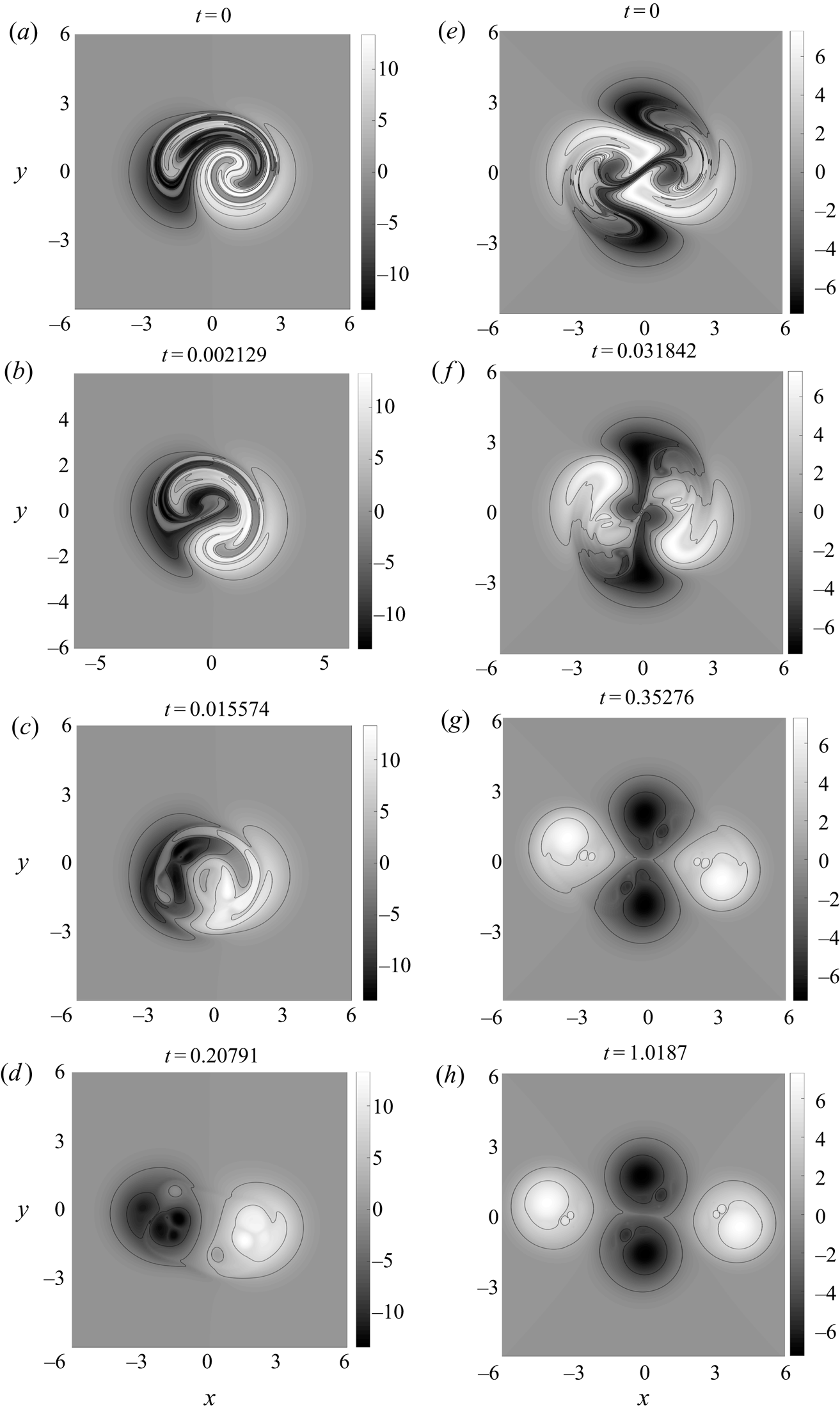
Figure 7. Pseudo-colour plot of  $f$ with four contour levels: (a–d) $\mathcal {T}=2$ case; (e–h) $\mathcal {T}=3$ case. (a,e) Initial density distribution $f_0=\mathcal {A}(x,y,0)$; (b,f) contours of $f$ become less elongated; (c,g) positive and negative regions separate; (d,h) the final unstirred scalar field $f_T$. Animated versions of the two columns of this figure are available in the supplementary material; see movies 1 and 2 available at https://doi.org/10.1017/jfm.2020.1154.
We apply MR and show the time evolution of  $f$ for both cases by the subsequent rows in figure 7. Only the central region $[-6, 6]\times [-6, 6]$ is shown for clarity. We see that the MR algorithm successfully separates the tangled patterns of $f_0$ into separate regions, and multiple extrema exist within each region. The density distribution around each local extremum becomes more circular in the relaxed solution. For the $\mathcal {T}=3$ case, the saddle point between the two negative regions in $f$ has collapsed to a line, also seen for simpler initial conditions by Linardatos (Reference Linardatos1993).
When it comes to large-scale features, for the  $\mathcal {T}=2$ case, there are two main regions in the final state $f_T$ (positive and negative), but for the $\mathcal {T}=3$ case, there are three regions (the positive region is split into two disconnected parts). We see that $\mathcal {T}$ controls not only the number of regions in the FLH but also the final state $f_T$ in our MR calculations. This is a direct consequence of preserving the topological structure of $f_0$. The fact that an analogous evolution happens in the 3-D simulations of Yeates et al. (Reference Yeates, Hornig and Wilmot-Smith2010) supports the idea that the FLH in the 3-D simulation evolves primarily by simplifying under advection (Russell et al. Reference Russell, Yeates, Hornig and Wilmot-Smith2015; Pontin et al. Reference Pontin, Candelaresi, Russell and Hornig2016). For the $\mathcal {T}=2$ case, we can also directly compare figures 1(d–f) and 7.
During the unstirring, the velocity field  $\boldsymbol {u}$ determined by the MR algorithm adapts to the patterns of $f$ at every time step. This is illustrated by the vector plots in figure 8 with the contours of $f$ in the background. The unstirring occurs mostly in regions where $f$ is ‘folded’ and is less relevant around the edges of the domain. Interestingly, we observe that $\boldsymbol {u}$ has the same topology as $f$, in the following sense. We can assign a topological degree to $\boldsymbol {u}$ as the number of vortex centres (O-points) minus the number of stagnation points (X-points). This number is observed to match the equivalent number computed from the critical points of the scalar field $f$, which for these simulations is $\mathcal {T}$.
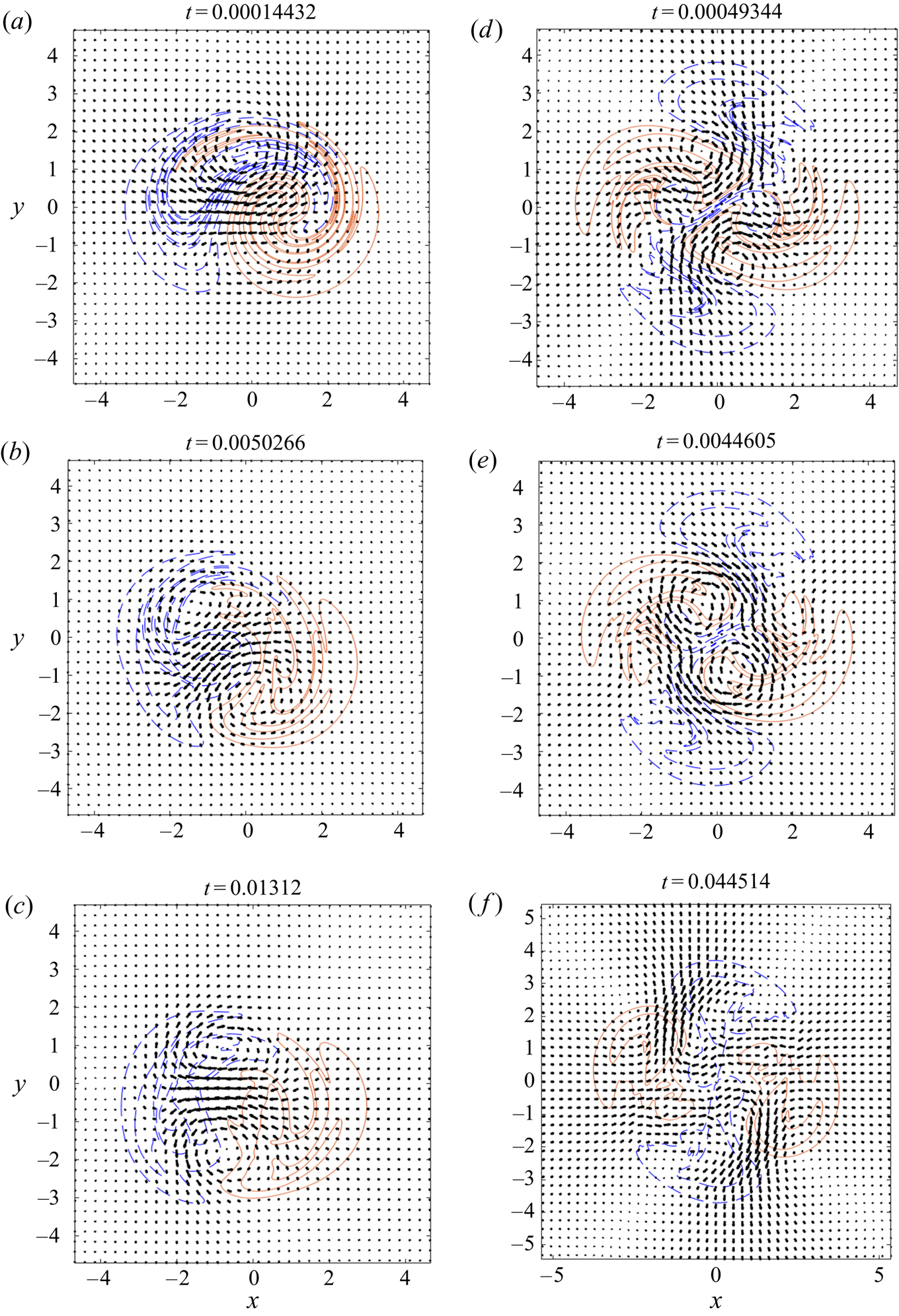
Figure 8. The obtained velocity field  $\boldsymbol {u}$ at different times superimposed on isocontours of $f$. Two contours with positive values are represented by red solid lines, and two contours with negative values are represented by dashed blue lines. As time goes by, $\boldsymbol {u}$ gradually unfolds $f$. An animated version of this figure is available in the supplementary material; see movies 3 and 4. (a–c) The $\mathcal {T}=2$ case. (d–f) The $\mathcal {T}=3$ case.
Next we show some diagnostics of the MR process. The energy  $E(t)=\langle |\boldsymbol {\nabla } f|^2\rangle$ and the enstrophy $\varepsilon (t)=\langle |\boldsymbol {\nabla }\times \boldsymbol {u}|^2\rangle$ as functions of time are shown in figure 9. In both test cases, the energy converges to an asymptotic value. The enstrophy is expected to converge towards zero from (2.21). Numerically we find a ${O}(10^5)$ magnitude drop. Additionally, the signature function $\mathcal {S}(f_c)$ and the histogram of $f$ values at each grid point for $f_0$ and $f_T$ are well conserved, shown in figures 10 and 11. For the signature function, the isocontours $f_c$ are taken at $200$ equally spaced points in the range $[f_{min}, f_{max}]$. The histogram is sampled in the same reduced domain as in figure 7. Together, these measures show that the topology of $f$ is well preserved during MR.
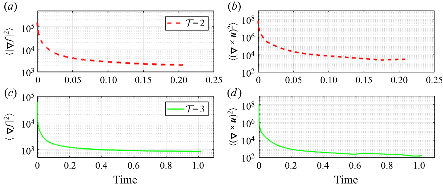
Figure 9. Energy  $E(t)=\langle |\boldsymbol {\nabla } f(x,y,t)|^2\rangle$ and enstrophy $\varepsilon (t)=\langle |\boldsymbol {\nabla }\times \boldsymbol {u}(x,y,t)|^2\rangle$ as functions of time.
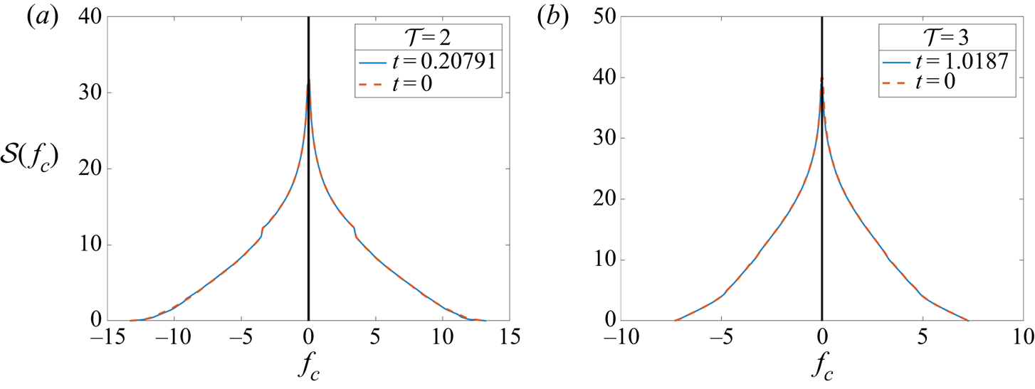
Figure 10. Comparison of signature functions  $\mathcal {S}(f_c)$ for non-zero values of $f_0$ and $f_T$.
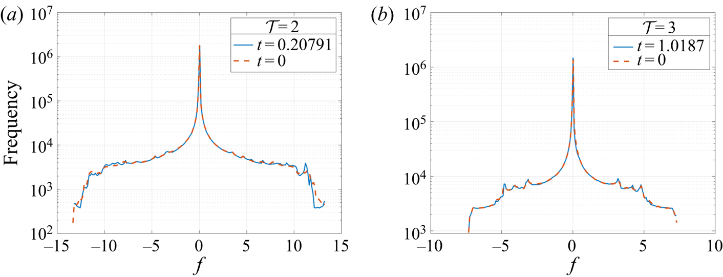
Figure 11. Comparison of histograms of  $f_0$ and $f_T$ sampled from the same plot windows as in figure 7.
4. Conclusion
In this study, we sought to determine the simplest final state  $f_T$ of a passive scalar field that could be obtained by incompressible advection. Two types of method were tested: the adjoint-based VM that either minimises the Dirichlet seminorm $E(t)=\langle |\boldsymbol {\nabla } f|^2\rangle$ directly (parametrised by $\theta =1$), or maximises a mix-norm measured by $\langle |\nabla ^{-1} f|^2\rangle$ (parametrised by $\theta =-1$); and the 2-D MR driven by a fictitious force $-\nabla ^2 f(\boldsymbol {\nabla } f)$, which guarantees a monotonic decrease in $E(t)$. VM has the theoretical advantage of imposing fewer a priori restrictions on the unstirring velocity field, and VM ( $\theta =-1$) is numerically more stable than VM ( $\theta =1$). This is consistent with previous studies using mix-norms (Thiffeault Reference Thiffeault2012; Foures et al. Reference Foures, Caulfield and Schmid2014; Marcotte & Caulfield Reference Marcotte and Caulfield2018). VM is also adaptable in ways that MR is not: for example, if one were to consider a more restricted problem requiring that the velocity field satisfies the Navier–Stokes equations. However, VM ( $\theta =-1$) becomes computationally expensive, and struggles to converge when $f_0$ gets complex. Hence, we found MR to be the preferred method for general initial conditions, since it is numerically more robust and scalable than VM.
Having identified our preferred method for complex initial conditions, we applied it to the FLH patterns of 3-D magnetic braids. Our main objective in doing so was to probe the governing principles of the 3-D simulations; specifically, could simplifying the pattern of the FLH under passive advection determine the final magnetic field produced by 3-D turbulent magnetic reconnection? The results in this paper agree with the 3-D simulations, in that  $f$ separates into a small number of large-scale regions with positive or negative FLH, with the same topological degree as the initial configuration (cf. Yeates et al. Reference Yeates, Russell and Hornig2015). This finding supports the idea that the dominant evolution of the FLH, at least at large scales, is pure advection.
An interesting difference between the optimal unstirred states found in this work and the FLH distributions produced by 3-D magnetic reconnection is that the large-scale regions produced by pure advection still contain topological substructure in the contours of  $f$ (for example in figure 7d). There are several local maxima/minima within the main positive and negative regions, because the topology of contours and critical points is preserved under advection. Previously published 3-D magnetic reconnection simulations – like in figure 1(f) – have not shown this substructure in the final FLH (Yeates et al. Reference Yeates, Hornig and Wilmot-Smith2010; Pontin et al. Reference Pontin, Candelaresi, Russell and Hornig2016). The evolution equation (1.3) for the FLH derived by Russell et al. (Reference Russell, Yeates, Hornig and Wilmot-Smith2015) contains other terms in addition to the advection term. In principle, these terms allow for further simplification of the substructure. The $\boldsymbol {w}\boldsymbol {\cdot }\boldsymbol {A}$ term is especially interesting from this point of view, and our findings motivate and support future investigations of its role. At the same time, it is also possible that this substructure is not seen in the 3-D simulations because the numerically accessible resistivity causes it to diffuse.
A natural question that arises from this study is how the MR method could be generalised to 3-D fluids. One idea is to choose the unstirring velocity to be a volume-preserving mean curvature flow (Huisken Reference Huisken1987). Such a flow has already been used to model the deformation of droplets (Thürey et al. Reference Thürey, Wojtan, Gross and Turk2010), though care would be needed at singularities (Mayer Reference Mayer2001). By contrast, the VM method generalises naturally to three dimensions, though its numerical implementation would be a significant challenge.
To conclude, our study shows that MR provides a powerful method for unstirring a scalar field, even if the original scalar has nothing to do with magnetic fields. We have shown that the method can work well for configurations much more complex than the pioneering numerical studies of Linardatos (Reference Linardatos1993), while reproducing the expected tendencies of contours to become ‘simpler’ and of saddle points to degenerate into Y-type line singularities (Linardatos Reference Linardatos1993; Arnold & Khesin Reference Arnold and Khesin1998). The most obvious example of the latter is between the negative regions at the end of the  $\mathcal {T}=3$ simulation (figure 7). The strength of MR lies in its prescription of a specific velocity field that is guaranteed to efficiently unstir $f$, in the sense that the Dirichlet seminorm is monotonically decreasing. While such a velocity field may be challenging to generate in real fluids, it could in principle be imposed in a conducting fluid by appropriate control of the electric current density. It could be used more readily as an unstirring method in computational studies.
Supplementary movies
Supplementary movies are available at https://doi.org/10.1017/jfm.2020.1154.
Acknowledgements
We thank G. Hornig and P. Wyper for useful discussions during this research, as well as the anonymous referees for significantly improving the paper.
Funding
This work was supported by Leverhulme Trust grant PRG-2017-169.
Declaration of interests
The authors report no conflict of interest.
Appendix A. Variations of the Lagrangian
Here we show explicitly the variational derivatives of the Lagrangian  $\mathcal {L}$ given by (2.7). We assume either periodic boundary conditions on $f$ and $\boldsymbol {u}$, or $\boldsymbol {\nabla } f|_{\partial D}=0$ and impermeable boundary conditions on $\boldsymbol {u}$ ( $\boldsymbol {u}\boldsymbol {\cdot } \boldsymbol {n}|_{\partial D}=0$). For clarity, we take the case $\theta =1$. Firstly, to derive the variations with respect to $f$ and $f_T$, we rewrite the Lagrangian as
 \begin{align} {\mathcal{L}} &={-}\langle\, f_T\nabla^2 f_T\rangle +\oint_{\partial D} f_T\,\boldsymbol{n}\boldsymbol{\cdot}\boldsymbol{\nabla} f_T \,\text{d} l + \langle \varPi\boldsymbol{\nabla}\boldsymbol{\cdot}\boldsymbol{u}\rangle\nonumber\\ &\quad -\int_0^T\left\langle\left(\frac{\partial \varGamma}{\partial t}+\boldsymbol{u}\boldsymbol{\cdot}\boldsymbol{\nabla} \varGamma+\varGamma (\boldsymbol{\nabla}\boldsymbol{\cdot}\boldsymbol{u})\right) f \right\rangle\,\text{d} t +\left.\langle\varGamma f\rangle\right\rvert_0^T+\int_0^T\oint_{\partial D} \varGamma(\boldsymbol{u}\boldsymbol{\cdot}\boldsymbol{n})f \,\text{d} l \,\text{d} t \nonumber\\ &={-}\langle f_T\nabla^2 f_T\rangle +\langle \varPi\boldsymbol{\nabla}\boldsymbol{\cdot}\boldsymbol{u}\rangle -\int_0^T\left\langle\left(\frac{\partial \varGamma}{\partial t} +(\boldsymbol{u}\boldsymbol{\cdot}\boldsymbol{\nabla} )\varGamma+\varGamma(\boldsymbol{\nabla}\boldsymbol{\cdot}\boldsymbol{u})\right) f \right\rangle\,\text{d} t \nonumber\\ &\quad +\langle\varGamma_T f_T-\varGamma_0 f_0\rangle, \end{align}
where the contour integral along the boundary vanishes because of the boundary conditions on  $f$ and $\boldsymbol {u}$ mentioned above. Similarly, since
 \begin{gather} {-}\langle f_T\nabla^2 \delta f_T\rangle= \langle \boldsymbol{\nabla} f_T\boldsymbol{\cdot}\boldsymbol{\nabla} \delta f_T\rangle-\oint_{\partial D} f_T\,\boldsymbol{n}\boldsymbol{\cdot}\boldsymbol{\nabla} \delta f_T \,\text{d} l\nonumber\\ ={-}\langle \nabla^2 f_T\delta f_T\rangle+\oint_{\partial D}\boldsymbol{\nabla} f_T\boldsymbol{n}\boldsymbol{\cdot}\boldsymbol{\nabla} \delta f_T \,\text{d} l-\oint_{\partial D} f_T\boldsymbol{n}\boldsymbol{\cdot}\boldsymbol{\nabla} \delta f_T \,\text{d} l\nonumber\\ ={-}\langle \delta f_T\nabla^2 f_T\rangle, \end{gather}
the variational derivatives with respect to  $f_T$ and $f$ are
 \begin{gather} \frac{\delta{\mathcal{L}}}{\delta f_T} ={-}2\nabla^2 f_T+\varGamma_T, \end{gather}
 \begin{gather}\frac{\delta{\mathcal{L}}}{\delta f} ={-}\left(\frac{\partial \varGamma}{\partial t} +(\boldsymbol{u}\boldsymbol{\cdot}\boldsymbol{\nabla}) \varGamma+\varGamma(\boldsymbol{\nabla}\boldsymbol{\cdot}\boldsymbol{u}) \right). \end{gather}
 To get the variation with respect to  $\boldsymbol {u}$, we need to rewrite the Lagrangian as follows:
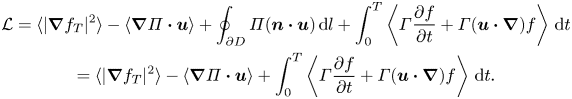 \begin{gather} {\mathcal{L}} = \langle |\boldsymbol{\nabla} f_T|^2\rangle -\langle\boldsymbol{\nabla} \varPi\boldsymbol{\cdot}\boldsymbol{u}\rangle +\oint_{\partial D} \varPi (\boldsymbol{n}\boldsymbol{\cdot}\boldsymbol{u}) \,\text{d} l+\int_0^T\left\langle \varGamma\frac{\partial f}{\partial t} +\varGamma(\boldsymbol{u}\boldsymbol{\cdot}\boldsymbol{\nabla}) f \right\rangle \,\text{d} t \nonumber\\ =\langle |\boldsymbol{\nabla} f_T|^2\rangle -\langle\boldsymbol{\nabla} \varPi\boldsymbol{\cdot}\boldsymbol{u}\rangle +\int_0^T\left\langle \varGamma\frac{\partial f}{\partial t} +\varGamma(\boldsymbol{u}\boldsymbol{\cdot}\boldsymbol{\nabla}) f \right\rangle\,\text{d} t. \end{gather}
The velocity field is steady so we can take it out of the integral, and then (A5) becomes
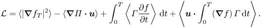 \begin{equation} {\mathcal{L}}=\langle |\boldsymbol{\nabla} f_T|^2\rangle -\langle\boldsymbol{\nabla} \varPi\boldsymbol{\cdot}\boldsymbol{u}\rangle +\int_0^T\left\langle \varGamma\frac{\partial f}{\partial t} \right\rangle\,\text{d} t +\left\langle\boldsymbol{u}\boldsymbol{\cdot}\int_0^T(\boldsymbol{\nabla} f )\,\varGamma\,\text{d} t\right\rangle. \end{equation}
Hence, the variational derivative with respect to  $\boldsymbol {u}$ is
 \begin{equation} \frac{\delta{\mathcal{L}}}{\delta \boldsymbol{u}} ={-}\boldsymbol{\nabla}\varPi +\int_0^T(\boldsymbol{\nabla} f) \varGamma\,\text{d} t. \end{equation}
The two trivial variational derivatives give back the constraints we impose:
 \begin{gather} \frac{\delta{\mathcal{L}}}{\delta\varPi} = \boldsymbol{\nabla}\boldsymbol{\cdot}\boldsymbol{u}, \end{gather}
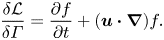 \begin{gather}\frac{\delta{\mathcal{L}}}{\delta\varGamma} =\frac{\partial f}{\partial t} +(\boldsymbol{u}\boldsymbol{\cdot}\boldsymbol{\nabla}) f. \end{gather}
 The derivation for the mix-norm ( $\theta =-1$) is similar. If we write $\nabla ^2\phi = f_T$, then $\phi =\nabla ^{-2} f_T$, so we get $\boldsymbol {\nabla }\phi =\boldsymbol {\nabla }\nabla ^{-2} f_T=\nabla ^{-1} f_T$, as in Foures et al. (Reference Foures, Caulfield and Schmid2014) and Marcotte & Caulfield (Reference Marcotte and Caulfield2018). The objective functional can then be rewritten as
 \begin{equation} \langle |\nabla^{{-}1} f_T|^2\rangle = \langle|\boldsymbol{\nabla}\phi|^2 \rangle={-}\langle \phi\nabla^2 \phi\rangle + \oint_{\partial D}\phi\,\boldsymbol{n}\boldsymbol{\cdot}\boldsymbol{\nabla} \phi \,\text{d} l ={-}\langle (\nabla^{{-}2} f_T)f_T \rangle, \end{equation}
where we assumed periodic boundary conditions for  $\phi$, and the variational derivatives for $f_T$ and $f$ are
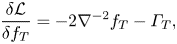 \begin{gather} \frac{\delta{\mathcal{L}}}{\delta f_T} ={-}2\nabla^{{-}2} f_T-\varGamma_T, \end{gather}
 \begin{gather}\frac{\delta{\mathcal{L}}}{\delta f} =\frac{\partial \varGamma}{\partial t} +(\boldsymbol{u}\boldsymbol{\cdot}\boldsymbol{\nabla}) \varGamma+\varGamma(\boldsymbol{\nabla}\boldsymbol{\cdot}\boldsymbol{u}). \end{gather}
Appendix B. Initial patterns for § 3
Our initial  $f_0$ patterns are based on the $\mathcal {T}=2$ and $\mathcal {T}=3$ configurations simulated in three dimensions by Yeates et al. (Reference Yeates, Hornig and Wilmot-Smith2010). Those initial configurations were braided magnetic fields in a 3-D Cartesian domain with the general form
 \begin{align} \boldsymbol{B}_0(x,y,z) &= \hat{\boldsymbol{z}}+\sum_{i=1}^n \frac{ 2 k_i}{\sqrt{2}}\left[-(y-y_i)\hat{\boldsymbol{x}}+(x-x_i)\hat{\boldsymbol{y}}\right]\nonumber\\ &\qquad\quad \times \exp \left[-\frac{(x-x_i)^2+(y-y_i)^2}{2}-\frac{(z-z_i)^2}{4}\right]. \end{align}
The case with topological degree  $\mathcal {T}=2$, also called the E3 braid, has parameters $n=6$, $k_i=x_i=[1, -1, 1, -1, 1, -1]$, $y_i=[0, 0, 0, 0, 0, 0]$ and $z_i=[-20, -12, -4, 4, 12, 20]$. The case with topological degree $\mathcal {T}=3$ has parameters $n=8$, $k_i=[1, 1, -1,-1, 1, 1, -1$, $-1 ]$, $x_i=1.27[1, -1, 0, 0, 1,-1, 0, 0]$, $y_i=1.27[0, 0, 1, -1, 0, 0, 1,-1]$ and $z_i=[-18, -18, -6,-6, 6, 6, 18, 18]$.
We set our initial 2-D scalar field  $f_0$ to the FLH pattern of the corresponding magnetic field, as defined in (1.2). Since each field line connects from the lower boundary $z=-24$ to the upper boundary $z=24$, we can view $\mathcal {A}$ as a scalar function on any cross-section – here, we take the lower boundary $z=-24$, and set $f_0(x,y)=\mathcal {A}(x,y,0)$. The resulting patterns are shown in the top row of figure 7.


 Open access