


1 Introduction
Obstructions for topological objects to have geometric structures are important subjects of study in topology and geometry. For example, the geometrization theorem is about topological obstructions for a 3-manifold to have one out of eight geometries. W. Thurston, who conjectured and proved a large part of the geometrization theorem, also proved a geometrization theorem, named Thurston’s characterization, in complex dynamics. He found obstructions, called Thurston obstructions, for a post-critically finite branched covering of the $2$
-sphere to be isotopic to a rational map [Reference Douady and HubbardDH93]. Levy cycles were introduced at first as simple cases of Thurston obstructions in the study of the mating problem [Reference LevyLev85, Reference TanTan92]. Recently, it turned out that a Levy cycle itself is an obstruction for a post-critically finite branched covering to be isotopic to an expanding dynamical system [Reference Bartholdi and DudkoBD18]. Therefore, it is important to determine the existence of a Levy cycle as well as a Thurston obstruction for post-critically finite branched coverings. In this paper, we investigate a new method to detect the existence of a Levy cycle for a broad family of branched coverings, called subdivision maps of finite subdivision rules.
$2$
-sphere to be isotopic to a rational map [Reference Douady and HubbardDH93]. Levy cycles were introduced at first as simple cases of Thurston obstructions in the study of the mating problem [Reference LevyLev85, Reference TanTan92]. Recently, it turned out that a Levy cycle itself is an obstruction for a post-critically finite branched covering to be isotopic to an expanding dynamical system [Reference Bartholdi and DudkoBD18]. Therefore, it is important to determine the existence of a Levy cycle as well as a Thurston obstruction for post-critically finite branched coverings. In this paper, we investigate a new method to detect the existence of a Levy cycle for a broad family of branched coverings, called subdivision maps of finite subdivision rules.
1.1 Obstructions of post-critically finite topological branched self-coverings of the sphere
A continuous map $f:S^2 \rightarrow S^2$
is a topological branched covering if it locally looks like
$f:S^2 \rightarrow S^2$
is a topological branched covering if it locally looks like $z \mapsto z^d$
for some integer
$z \mapsto z^d$
for some integer $d>0$
. A point
$d>0$
. A point $x \in S^2$
is a critical point if f is not locally injective at x. The collection of the critical points
$x \in S^2$
is a critical point if f is not locally injective at x. The collection of the critical points $\Omega _f$
is the critical set of f and its forward orbit
$\Omega _f$
is the critical set of f and its forward orbit $P_f:=\bigcup _{k=1}^\infty f^{\circ k}(\Omega _f)$
is the post-critical set. If
$P_f:=\bigcup _{k=1}^\infty f^{\circ k}(\Omega _f)$
is the post-critical set. If $P_f$
is finite, f is a post-critically finite branched covering, or simply a Thurston map. A marked post-critically finite branched covering is a map
$P_f$
is finite, f is a post-critically finite branched covering, or simply a Thurston map. A marked post-critically finite branched covering is a map ![]() such that
such that $A \supset P_f$
,
$A \supset P_f$
, $|A|<\infty $
, and
$|A|<\infty $
, and $f(A) \subset A$
. Every element
$f(A) \subset A$
. Every element $a\in A$
is called a marked point and A is called the set of marked points of
$a\in A$
is called a marked point and A is called the set of marked points of ![]() . Since
. Since ![]() contains the information of being post-critically finite and the set of marked points, we often abbreviate it just as a branched covering and write more words when they are necessary.
contains the information of being post-critically finite and the set of marked points, we often abbreviate it just as a branched covering and write more words when they are necessary.
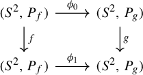
Two branched coverings ![]() and
and ![]() are combinatorially equivalent (by
are combinatorially equivalent (by $\phi _0$
and
$\phi _0$
and $\phi _1$
) if there exist homeomorphisms
$\phi _1$
) if there exist homeomorphisms $\phi _0,\phi _1:(S^2,A) \rightarrow (S^2,B)$
such that: (1)
$\phi _0,\phi _1:(S^2,A) \rightarrow (S^2,B)$
such that: (1) $\phi _0(A)=\phi _1(A)=B$
; (2)
$\phi _0(A)=\phi _1(A)=B$
; (2) $\phi _1$
is homotopic relative to A to
$\phi _1$
is homotopic relative to A to $\phi _0$
; and (3) the following diagram commutes:
$\phi _0$
; and (3) the following diagram commutes:
A post-critically finite topological branched covering which is not doubly covered by a torus endomorphism is combinatorially equivalent to a post-critically finite rational map if and only if it does not have a Thurston obstruction [Reference Douady and HubbardDH93], see §7.1.
Definition 1.1. (Levy cycle)
A Levy cycle, or a Levy obstruction, of a post-critically finite branched covering ![]() is a collection of simple closed curves
is a collection of simple closed curves $\{\gamma _1,\gamma _2,\ldots ,\gamma _n\}$
that are essential relative to A with the following property: for each
$\{\gamma _1,\gamma _2,\ldots ,\gamma _n\}$
that are essential relative to A with the following property: for each $1\le i \le n$
, there is a connected component
$1\le i \le n$
, there is a connected component $\gamma _i^{\prime }$
of
$\gamma _i^{\prime }$
of $f^{-1}(\gamma _i)$
which is isotopic to
$f^{-1}(\gamma _i)$
which is isotopic to $\gamma _{i+1}$
relative to A, and
$\gamma _{i+1}$
relative to A, and $f|_{\gamma _i^{\prime }}:\gamma _i^{\prime } \to \gamma _i$
is a homeomorphism.
$f|_{\gamma _i^{\prime }}:\gamma _i^{\prime } \to \gamma _i$
is a homeomorphism.
Since a Levy cycle is a homeomorphically periodic cycle, a branched covering cannot be expanding along a Levy cycle. The Schwartz lemma implies that every post-critically finite rational map ![]() is expanding with respect to the conformal metric on
is expanding with respect to the conformal metric on $\hat {\mathbb {C}} \setminus P_g$
, except for a few cases. Therefore, a Levy cycle is an example of a Thurston obstruction. Shishikura and Tan found an example of mating of cubic polynomials that has a Thurston obstruction but does not have a Levy cycle [Reference Shishikura and TanST00]. Although Shishikura and Tan’s example is not conjugate to a rational map, it has an expanding metric, and many objects in the study of rational maps, such as Julia sets, are still well defined. These branched coverings are called Böttcher expanding maps, see [Reference Bartholdi and DudkoBD18] for Böttcher expanding maps. Rational maps are Böttcher expanding maps by the Schwartz lemma. Recently, it was shown that a post-critically finite topological branched covering which is not doubly covered by a torus endomorphism is combinatorially equivalent to a Böttcher expanding map if and only if it does not have a Levy cycle [Reference Bartholdi and DudkoBD18]. Therefore, Thurston and Levy obstructions can be viewed as obstructions for conformal structures and expanding dynamics on branched coverings of the sphere, respectively.
$\hat {\mathbb {C}} \setminus P_g$
, except for a few cases. Therefore, a Levy cycle is an example of a Thurston obstruction. Shishikura and Tan found an example of mating of cubic polynomials that has a Thurston obstruction but does not have a Levy cycle [Reference Shishikura and TanST00]. Although Shishikura and Tan’s example is not conjugate to a rational map, it has an expanding metric, and many objects in the study of rational maps, such as Julia sets, are still well defined. These branched coverings are called Böttcher expanding maps, see [Reference Bartholdi and DudkoBD18] for Böttcher expanding maps. Rational maps are Böttcher expanding maps by the Schwartz lemma. Recently, it was shown that a post-critically finite topological branched covering which is not doubly covered by a torus endomorphism is combinatorially equivalent to a Böttcher expanding map if and only if it does not have a Levy cycle [Reference Bartholdi and DudkoBD18]. Therefore, Thurston and Levy obstructions can be viewed as obstructions for conformal structures and expanding dynamics on branched coverings of the sphere, respectively.
1.2 Analogy with surface diffeomorphisms
There are analogues between surface diffeomorphisms and branched coverings of the sphere. Pseudo-Anosov maps are geometric in a sense that they are affine maps expanding along one dimension and contracting along the other one dimension with respect to appropriate conned Euclidean structures; rational maps are conformal geometric and Böttcher expanding maps are metric geometrically defined. In a pseudo-Anosov mapping class, there is a unique pseudo-Anosov map up to conjugation; in an isotopy class of post-critically finite topological branched coverings, a rational map or a Böttcher expanding map is unique up to conjugation if it exists [Reference Bartholdi and DudkoBD18, Reference Douady and HubbardDH93]. For non-periodic mapping classes, reducing multicurves are obstructions to pseudo-Anosov mapping classes; Thurston obstructions and Levy cycles are also multicurves, which are obstructions to being isotopic to rational maps and Böttcher expanding maps, respectively.
In spite of this analogy, however, algorithms to determine the existence of obstructions for branched coverings of the sphere are relatively less studied compared with surface diffeomorphisms. Let us review some results on algorithms about branched coverings of the sphere. Exhaustive searches for Levy cycles or Thurston obstructions are decidable [Reference Bonnot, Braverman and YampolskyBBY12, Reference Bartholdi and DudkoBD18]. For topological polynomials, a non-exhaustive algorithm, which finds either Levy cycles if they exist or Hubbard trees otherwise, was developed in [Reference Belk, Lanier, Margalit and WinarskiBLMW22]. D. Thurston’s positive characterization also gives a non-exhaustive algorithm to detect both Levy cycles and Thurston obstructions for hyperbolic post-critically finite branched coverings [Reference ThurstonThu20]. Although these algorithms work efficiently for many examples in practice, no theoretical upper bound of the complexity is known for any of these algorithms. An upper bound for the computational complexity was studied for nearly Euclidean Thurston maps in [Reference Floyd, Parry and PilgrimFPP18a]. Poirier proved that an abstract Hubbard tree H is a Hubbard tree of a polynomial if and only if H is expanding [Reference PoirierPoi10]. This gives an efficient algorithm to check whether a Thurston obstruction (equivalently a Levy cycle in this case) exists, and one can easily find an upper bound for the complexity of this algorithm, though it is not stated in [Reference PoirierPoi10]. In this paper, Theorem 6.21 provides a new non-exhaustive algorithm to detect Levy cycles when post-critically finite branched coverings are given as subdivision maps of finite subdivision rules. When edges have polynomial growth of subdivisions, Theorem 8.6 implies that this algorithm terminates very quickly, and the complexity is polynomial about the number of cells. However, we do not compute the complexity in this paper.
1.3 Finite subdivision rules
A finite subdivision rule $\mathcal {R}$
consists of a partition
$\mathcal {R}$
consists of a partition $S_{\mathcal {R}}$
of
$S_{\mathcal {R}}$
of $S^2$
into polygons and its subdivision
$S^2$
into polygons and its subdivision $\mathcal {R}(S_{\mathcal {R}})$
such that a subdivision map
$\mathcal {R}(S_{\mathcal {R}})$
such that a subdivision map $f:\mathcal {R}(S_{\mathcal {R}})\to S_{\mathcal {R}}$
is homeomorphic on each open cell, see Figure 1 for an example and §4 for a precise definition. One can also see a finite subdivision rule as a sort of Markov partition. Because
$f:\mathcal {R}(S_{\mathcal {R}})\to S_{\mathcal {R}}$
is homeomorphic on each open cell, see Figure 1 for an example and §4 for a precise definition. One can also see a finite subdivision rule as a sort of Markov partition. Because $P_f \subset \operatorname{Vert}(S_{\mathcal {R}})$
, the subdivision map is a post-critically finite topological branched covering. By iterating subdivisions, we have a further subdivision
$P_f \subset \operatorname{Vert}(S_{\mathcal {R}})$
, the subdivision map is a post-critically finite topological branched covering. By iterating subdivisions, we have a further subdivision $\mathcal {R}^n(S_{\mathcal {R}})$
and an iterated map
$\mathcal {R}^n(S_{\mathcal {R}})$
and an iterated map $f^n:\mathcal {R}^n(S_{\mathcal {R}}) \to S_{\mathcal {R}}$
for each
$f^n:\mathcal {R}^n(S_{\mathcal {R}}) \to S_{\mathcal {R}}$
for each $n \in \mathbb {N}$
. It is an open question to determine which topological post-critically finite branched coverings are isotopic to subdivision maps of finite subdivision rules. See §4.3 for a list of topological branched coverings that can be represented as subdivision maps.
$n \in \mathbb {N}$
. It is an open question to determine which topological post-critically finite branched coverings are isotopic to subdivision maps of finite subdivision rules. See §4.3 for a list of topological branched coverings that can be represented as subdivision maps.
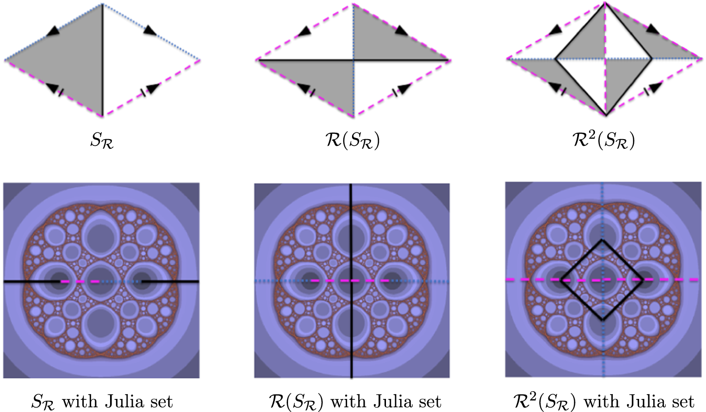
Figure 1 A finite subdivision rule of $z\mapsto ({z^2-1})/({z^2+1})$
. The sphere is decomposed into two triangles in
$z\mapsto ({z^2-1})/({z^2+1})$
. The sphere is decomposed into two triangles in $S_{\mathcal {R}}$
. Each triangle subdivides into two triangles under the subdivision
$S_{\mathcal {R}}$
. Each triangle subdivides into two triangles under the subdivision $\mathcal {R}$
. The subdivision map
$\mathcal {R}$
. The subdivision map $f:\mathcal {R}(S_{\mathcal {R}})\to S_{\mathcal {R}}$
sends each shaded or unshaded triangle in
$f:\mathcal {R}(S_{\mathcal {R}})\to S_{\mathcal {R}}$
sends each shaded or unshaded triangle in $\mathcal {R}(S_{\mathcal {R}})$
to the shaded or unshaded triangle in
$\mathcal {R}(S_{\mathcal {R}})$
to the shaded or unshaded triangle in $S_{\mathcal {R}}$
, respectively.
$S_{\mathcal {R}}$
, respectively.
To detect a Levy cycle, for each $n\ge 0$
, we define a level- n non-expanding spine
$n\ge 0$
, we define a level- n non-expanding spine $N^n$
which is a graph with a train-track structure encoding non-expanding parts of
$N^n$
which is a graph with a train-track structure encoding non-expanding parts of $\mathcal {R}^n(S_{\mathcal {R}})$
, see §6. A finite set
$\mathcal {R}^n(S_{\mathcal {R}})$
, see §6. A finite set $A\subset \operatorname{Vert}(S_{\mathcal {R}})$
is called a set of marked points of
$A\subset \operatorname{Vert}(S_{\mathcal {R}})$
is called a set of marked points of $\mathcal {R}$
if
$\mathcal {R}$
if $P_f\cup f(A)\subset A$
. A point
$P_f\cup f(A)\subset A$
. A point $a\in A$
is called a Fatou point if its forward orbit contains a periodic critical point. Otherwise,
$a\in A$
is called a Fatou point if its forward orbit contains a periodic critical point. Otherwise, $a\in A$
is called a Julia point. We say that the level-n non-expanding spine
$a\in A$
is called a Julia point. We say that the level-n non-expanding spine $N^n$
is essential relative to A if it contains (more precisely carries as a train-track) a closed curve that is homotopic relative to A neither to a point nor to some iterate of a peripheral loop of a Julia point in A.
$N^n$
is essential relative to A if it contains (more precisely carries as a train-track) a closed curve that is homotopic relative to A neither to a point nor to some iterate of a peripheral loop of a Julia point in A.
Theorem 6.21.
Let $\mathcal {R}$
be a finite subdivision rule and
$\mathcal {R}$
be a finite subdivision rule and $f:\mathcal {R}(S_{\mathcal {R}})\to S_{\mathcal {R}}$
be its subdivision map which is not doubly covered by a torus endomorphism. Let
$f:\mathcal {R}(S_{\mathcal {R}})\to S_{\mathcal {R}}$
be its subdivision map which is not doubly covered by a torus endomorphism. Let $A\subset \operatorname{Vert}(S_{\mathcal {R}})$
be a set of marked points, that is,
$A\subset \operatorname{Vert}(S_{\mathcal {R}})$
be a set of marked points, that is, $P_f \cup f(A)\subset A$
. Then the post-critically finite branched covering
$P_f \cup f(A)\subset A$
. Then the post-critically finite branched covering ![]() has a Levy cycle if and only if the level- n non-expanding spine
has a Levy cycle if and only if the level- n non-expanding spine $N^n$
is essential relative to A for every
$N^n$
is essential relative to A for every $n\ge 0$
.
$n\ge 0$
.
We first prove the equivalence between the existence of a Levy cycle and the existence of a sequence of curves with certain properties in §5 using the theory of self-similar groups. Then we show in §6 the equivalence between the existence of such a sequence of curves and the level-n non-expanding spine being essential at every level $n\ge 0$
.
$n\ge 0$
.
1.4 Algorithmic implication
Theorem 6.21 improves [Reference Bartholdi and DudkoBD18, Algorithm 5.5] by replacing the exhaustive semi-decidable search for nuclei of orbisphere bisets by checking if the non-expanding spines are essential, which terminates in finite time if there is no Levy cycle. There is an example showing that an arbitrarily higher level of non-expanding spine is required to be checked, see Proposition 9.9 in §9.3.
Question 1.2. Is there an upper bound function $U:\mathbb {Z}_+ \to \mathbb {Z}_+$
such that
$U:\mathbb {Z}_+ \to \mathbb {Z}_+$
such that ![]() has a Levy cycle if and only if
has a Levy cycle if and only if $N^n$
is essential relative to A for every
$N^n$
is essential relative to A for every $n<U(k)$
, where k is the number of tiles in
$n<U(k)$
, where k is the number of tiles in $\mathcal {R}$
?
$\mathcal {R}$
?
1.5 Finite subdivision rules with polynomial growth of subdivisions
We will see that the growth of the subdivision of an edge is either exponential or polynomial in Theorem 3.6 and Proposition 8.2. If every edge has polynomial growth of subdivisions, then the level-n non-expanding spines $N^n$
are independent of
$N^n$
are independent of $n \ge 0$
. Hence, the existence of a Levy cycle is decidable very quickly.
$n \ge 0$
. Hence, the existence of a Levy cycle is decidable very quickly.
Theorem 8.6.
Let $\mathcal {R}$
be a finite subdivision rule with polynomial growth of edge subdivisions and f be its subdivision map which is not doubly covered by a torus endomorphism. Let
$\mathcal {R}$
be a finite subdivision rule with polynomial growth of edge subdivisions and f be its subdivision map which is not doubly covered by a torus endomorphism. Let $A\subset \operatorname{Vert}(S_{\mathcal {R}})$
be a set of marked point, that is,
$A\subset \operatorname{Vert}(S_{\mathcal {R}})$
be a set of marked point, that is, $f(A) \cup P_f \subset A$
. Then the following are equivalent.
$f(A) \cup P_f \subset A$
. Then the following are equivalent.
-
(1) The branched covering
 does not have a Levy cycle.
 -
(2) The level-
$0$
non-expanding spine
$N^0$
is essential relative to A. -
(3) The branched covering
is combinatorially equivalent to a unique rational map up to conjugation by Möbius transformations.


1.6 Equivalence between Levy cycles and Thurston obstructions
Another important implication of Theorem 8.6 is the equivalence between the existence of a Levy cycle and the existence of a Thurston obstruction. As explained earlier, there are topological branched coverings which do not have a Levy cycle but have a Thurston obstruction [Reference Shishikura and TanST00]. For some families of post-critically finite topological branched coverings, e.g., post-critically finite topological polynomials or branched coverings of degree $2$
, the existence of a Thurston obstruction implies the existence of a Levy cycle, by Levy et al [Reference HubbardHub16, Reference TanTan92]. We add two new families to this list: subdivision maps with polynomial growth of edge subdivisions (Theorem 8.6) and matings of polynomials one of which has core entropy zero (Corollary 7.10).
$2$
, the existence of a Thurston obstruction implies the existence of a Levy cycle, by Levy et al [Reference HubbardHub16, Reference TanTan92]. We add two new families to this list: subdivision maps with polynomial growth of edge subdivisions (Theorem 8.6) and matings of polynomials one of which has core entropy zero (Corollary 7.10).
Corollary 7.10. Let f and g be post-critically finite hyperbolic (respectively possibly non-hyperbolic) polynomials such that at least one of f and g has core entropy zero. Then f and g are mateable if and only if the formal mating (respectively degenerate mating) does not have a Levy cycle.
The equivalence between the existence of a Levy cycle and of a Thurston obstruction follows from the graph intersecting obstruction theorem, which is a generalization of the arcs intersecting obstruction theorem by Pilgrim and Tan [Reference Pilgrim and TanPT98]. Here, $h_{\textrm {top}}$
indicates the topological entropy.
$h_{\textrm {top}}$
indicates the topological entropy.
Theorem 7.6. (Graph intersecting obstruction)
Let ![]() be a post-critically finite branched covering and G be a forward invariant graph such that
be a post-critically finite branched covering and G be a forward invariant graph such that $h_{\textrm {top}}(f|_G)=0$
. Then every irreducible Thurston obstruction intersecting G is a Levy cycle.
$h_{\textrm {top}}(f|_G)=0$
. Then every irreducible Thurston obstruction intersecting G is a Levy cycle.
1.7 Examples: Critically fixed anti-holomorphic maps
In §9, we define an orientation reversing finite subdivision rule with no edge subdivision from every $2$
-vertex-connected planar graph G. Then
$2$
-vertex-connected planar graph G. Then ![]() and
and ![]() are post-critically finite topological branched coverings, where
are post-critically finite topological branched coverings, where $\tau $
is an orientation-reversing automorphism of G. Then we show in Theorem 9.4 that these maps do not have Levy cycles (or equivalently, Thurston obstructions) if and only if G is
$\tau $
is an orientation-reversing automorphism of G. Then we show in Theorem 9.4 that these maps do not have Levy cycles (or equivalently, Thurston obstructions) if and only if G is $3$
-edge-connected. While this article was being written, two papers [Reference GeyerGey22, Reference Lodge, Lyubich, Merenkov and MukherjeeLLMM23] were published where it is shown that every critically fixed anti-holomorphic map is constructed in this way and a theorem almost the same as Theorem 9.4 is proved.
$3$
-edge-connected. While this article was being written, two papers [Reference GeyerGey22, Reference Lodge, Lyubich, Merenkov and MukherjeeLLMM23] were published where it is shown that every critically fixed anti-holomorphic map is constructed in this way and a theorem almost the same as Theorem 9.4 is proved.
1.8 Notation for integer intervals
We introduce a non-standard but intuitive notation for integer intervals to distinguish them from real intervals. For $a<b\in \mathbb {Z}$
:
$a<b\in \mathbb {Z}$
:
-
$\bullet $
$[a,b]_{\mathbb {Z}}:=\{a,a+1,\ldots , b\}$
;
-
$\bullet $
$[a,\infty ]_{\mathbb {Z}}:=\{a,a+1,\ldots \}\cup \{\infty \}$
;
-
$\bullet $
$[-\infty ,b]_{\mathbb {Z}}:=\{-\infty \} \cup \{\ldots {,}\,b-1,b\}$
;
-
$\bullet $
$[-\infty ,\infty ]_{\mathbb {Z}}:=\mathbb {Z}$
.


The interval $[a,b]$
without the subscript
$[a,b]$
without the subscript $_{\mathbb {Z}}$
indicates the real interval
$_{\mathbb {Z}}$
indicates the real interval $\{x\in \mathbb {R}~|~a\le x \le b\}$
.
$\{x\in \mathbb {R}~|~a\le x \le b\}$
.
2 Monotonicity of lengths under subdivisions
In this section, we see combinatorial properties of a CW-complex without dynamics. We follow some terminology defined in [Reference Floyd, Parry and PilgrimFPP18b]. Let $\mathcal {T}$
be a finite CW-complex structure on
$\mathcal {T}$
be a finite CW-complex structure on $S^2$
. An n-gon, or a polygon if n is not specified, is a two-dimensional CW-complex structure on the closed
$S^2$
. An n-gon, or a polygon if n is not specified, is a two-dimensional CW-complex structure on the closed $2$
-disc
$2$
-disc $D^2$
whose
$D^2$
whose $1$
-skeleton consists of n edges on
$1$
-skeleton consists of n edges on $\partial D^2$
. For every closed
$\partial D^2$
. For every closed $2$
-cell t of
$2$
-cell t of $\mathcal {T}$
, there is a polygon
$\mathcal {T}$
, there is a polygon $\textbf {t}$
and a characteristic map
$\textbf {t}$
and a characteristic map $\phi _t:\textbf {t} \to \mathcal {T}$
such that
$\phi _t:\textbf {t} \to \mathcal {T}$
such that $\phi _t$
is cell-wise homeomorphic and
$\phi _t$
is cell-wise homeomorphic and $\phi _t(\textbf {t})=t$
.
$\phi _t(\textbf {t})=t$
.
Definition 2.1. (Bands and bones)
A band of $\mathcal {T}$
is a triple
$\mathcal {T}$
is a triple $(t;e_1,e_2)$
, where t is a closed
$(t;e_1,e_2)$
, where t is a closed $2$
-cell, and
$2$
-cell, and $e_1$
and
$e_1$
and $e_2$
are edges on the boundary of t. We allow
$e_2$
are edges on the boundary of t. We allow $e_1=e_2(=e)$
only when two boundary edges of a polygon
$e_1=e_2(=e)$
only when two boundary edges of a polygon $\textbf {t}$
are identified to e by the characteristic map
$\textbf {t}$
are identified to e by the characteristic map $\phi _t:\textbf {t}\to \mathcal {T}$
. We say that
$\phi _t:\textbf {t}\to \mathcal {T}$
. We say that $e_1$
and
$e_1$
and $e_2$
are the sides of the band. The bone of
$e_2$
are the sides of the band. The bone of $(t;e_1,e_2)$
is the homotopy class (or ambiguously a representative of the class) of curves which are properly embedded into
$(t;e_1,e_2)$
is the homotopy class (or ambiguously a representative of the class) of curves which are properly embedded into $(t,\partial t)$
with endpoints on the interiors of
$(t,\partial t)$
with endpoints on the interiors of $e_1$
and
$e_1$
and $e_2$
(see Figure 2).
$e_2$
(see Figure 2).
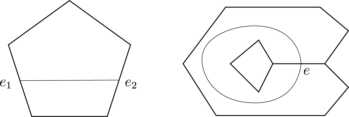
Figure 2 Bones of bands. The figure on the right shows the case when two sides of the band are the same.
Let $\mathcal {T}^{(n)}$
denote the n-skeleton of
$\mathcal {T}^{(n)}$
denote the n-skeleton of $\mathcal {T}$
. Any curve
$\mathcal {T}$
. Any curve $\gamma \subset S^2\setminus \mathcal {T}^{(0)}$
transverse to
$\gamma \subset S^2\setminus \mathcal {T}^{(0)}$
transverse to $\mathcal {T}^{(1)}$
is subdivided by
$\mathcal {T}^{(1)}$
is subdivided by $\mathcal {T}^{(1)}$
into consecutive subcurves
$\mathcal {T}^{(1)}$
into consecutive subcurves $\gamma _1,\gamma _2, \ldots ,\gamma _k$
such that each
$\gamma _1,\gamma _2, \ldots ,\gamma _k$
such that each $\gamma _i$
is a maximal subcurve embedded in a closed
$\gamma _i$
is a maximal subcurve embedded in a closed $2$
-cell. The set
$2$
-cell. The set $\{\gamma _1,\ldots ,\gamma _k\}$
is the
$\{\gamma _1,\ldots ,\gamma _k\}$
is the $\mathcal {T}$
-decomposition of
$\mathcal {T}$
-decomposition of $\gamma $
and each curve
$\gamma $
and each curve $\gamma _i$
is a
$\gamma _i$
is a $\mathcal {T}$
-segment of
$\mathcal {T}$
-segment of $\gamma $
.
$\gamma $
.
If $\gamma $
is not closed, then
$\gamma $
is not closed, then $\gamma _2,\ldots ,\gamma _{k-1}$
are called inner
$\gamma _2,\ldots ,\gamma _{k-1}$
are called inner $\mathcal {T}$
-segments. The terminal
$\mathcal {T}$
-segments. The terminal $\mathcal {T}$
-segment
$\mathcal {T}$
-segment $\gamma _1$
or
$\gamma _1$
or $\gamma _k$
is an outer
$\gamma _k$
is an outer $\mathcal {T}$
-segment if one of its endpoints is in the interior of a closed 2-cell; if both endpoints are on the 1-skeleton, then we still call them inner
$\mathcal {T}$
-segment if one of its endpoints is in the interior of a closed 2-cell; if both endpoints are on the 1-skeleton, then we still call them inner $\mathcal {T}$
-segments. If
$\mathcal {T}$
-segments. If $\gamma $
is closed, all segments are called inner segments. A curve
$\gamma $
is closed, all segments are called inner segments. A curve $\gamma $
is
$\gamma $
is $\mathcal {T}$
-taut if every inner
$\mathcal {T}$
-taut if every inner $\mathcal {T}$
-segment is the bone of a band, that is, it cannot be pushed away from the
$\mathcal {T}$
-segment is the bone of a band, that is, it cannot be pushed away from the $2$
-cell, it is contained by an isotopy relative to
$2$
-cell, it is contained by an isotopy relative to $\mathcal {T}^{(0)}$
.
$\mathcal {T}^{(0)}$
.
Definition 2.2. Two curves in $S^2\setminus \mathcal {T}^{(0)}$
are combinatorially equivalent relative to
$S^2\setminus \mathcal {T}^{(0)}$
are combinatorially equivalent relative to $\mathcal {T}$
, or simply
$\mathcal {T}$
, or simply $\mathcal {T}$
-combinatorially equivalent, if they are isotopic by a cellular isotopy of
$\mathcal {T}$
-combinatorially equivalent, if they are isotopic by a cellular isotopy of $\mathcal {T}$
, that is, an isotopy from the identity map whose restriction to each cell X is also an isotopy on X.
$\mathcal {T}$
, that is, an isotopy from the identity map whose restriction to each cell X is also an isotopy on X.
Define the $\mathcal {T}$
-length of
$\mathcal {T}$
-length of $\gamma $
, denoted by
$\gamma $
, denoted by $l_{\mathcal {T}}(\gamma )$
, to be the number of inner
$l_{\mathcal {T}}(\gamma )$
, to be the number of inner $\mathcal {T}$
-segments. The
$\mathcal {T}$
-segments. The $\mathcal {T}$
-length of a curve is an invariant of a combinatorial equivalence class. The following criterion is straightforward from the bigon criterion [Reference Farb and MargalitFM12].
$\mathcal {T}$
-length of a curve is an invariant of a combinatorial equivalence class. The following criterion is straightforward from the bigon criterion [Reference Farb and MargalitFM12].
Proposition 2.3. Let $\mathcal {T}$
be a finite CW-complex structure on
$\mathcal {T}$
be a finite CW-complex structure on $S^2$
. Let
$S^2$
. Let $\gamma $
be a curve in
$\gamma $
be a curve in $S^2\setminus \mathcal {T}^{(0)}$
transverse to
$S^2\setminus \mathcal {T}^{(0)}$
transverse to $\mathcal {T}^{(1)}$
. Then
$\mathcal {T}^{(1)}$
. Then $l_{\mathcal {T}}(\gamma )$
is minimized in its homotopy class within
$l_{\mathcal {T}}(\gamma )$
is minimized in its homotopy class within $S^2\setminus \mathcal {T}^{(0)}$
, relative to endpoints if
$S^2\setminus \mathcal {T}^{(0)}$
, relative to endpoints if $\gamma $
is not closed, if and only if
$\gamma $
is not closed, if and only if $\gamma $
is taut. Moreover, in the homotopy class, the taut curve is unique up to
$\gamma $
is taut. Moreover, in the homotopy class, the taut curve is unique up to $\mathcal {T}$
-combinatorial equivalence.
$\mathcal {T}$
-combinatorial equivalence.
The following lemma is immediate.
Lemma 2.4. Let $\mathcal {T}$
be a finite CW-complex structure on
$\mathcal {T}$
be a finite CW-complex structure on $S^2$
. For every
$S^2$
. For every $l>0$
, there are only finitely many, possibly closed or non-closed, curves
$l>0$
, there are only finitely many, possibly closed or non-closed, curves $\delta $
in
$\delta $
in $S^2\setminus \mathcal {T}^{(0)}$
with
$S^2\setminus \mathcal {T}^{(0)}$
with $l_{\mathcal {T}}(\delta )<l$
up to combinatorial equivalence relative to
$l_{\mathcal {T}}(\delta )<l$
up to combinatorial equivalence relative to $\mathcal {T}$
.
$\mathcal {T}$
.
Definition 2.5. (Subbands)
Assume $\mathcal {T}$
is a finite CW-complex structure on
$\mathcal {T}$
is a finite CW-complex structure on $S^2$
and
$S^2$
and $\mathcal {T}'$
is its subdivision. A band
$\mathcal {T}'$
is its subdivision. A band $(t';e^{\prime }_1,e^{\prime }_2)$
of
$(t';e^{\prime }_1,e^{\prime }_2)$
of $\mathcal {T}'$
is a subband of
$\mathcal {T}'$
is a subband of $(t;e_1,e_2)$
of
$(t;e_1,e_2)$
of $\mathcal {T}$
if
$\mathcal {T}$
if $t' \subset t$
and
$t' \subset t$
and $e_i^{\prime } \subset e_i$
for
$e_i^{\prime } \subset e_i$
for $i=1,2$
.
$i=1,2$
.
Proposition 2.6. (Monotonicity of lengths under refinements of CW-complexes)
Let $\mathcal {T}$
and
$\mathcal {T}$
and $\mathcal {T}'$
be finite CW-complex structures of the
$\mathcal {T}'$
be finite CW-complex structures of the $2$
-sphere
$2$
-sphere $S^2$
such that
$S^2$
such that $\mathcal {T}'$
is a subdivision of
$\mathcal {T}'$
is a subdivision of $\mathcal {T}$
. Let
$\mathcal {T}$
. Let $\gamma $
be a
$\gamma $
be a $\mathcal {T}$
-taut curve and
$\mathcal {T}$
-taut curve and $\gamma '$
be a
$\gamma '$
be a $\mathcal {T}'$
-taut curve such that
$\mathcal {T}'$
-taut curve such that $\gamma $
and
$\gamma $
and $\gamma '$
are
$\gamma '$
are $\mathcal {T}$
-combinatorially equivalent. Then
$\mathcal {T}$
-combinatorially equivalent. Then
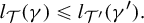 $$ \begin{align*} l_{\mathcal{T}}(\gamma) \le l_{\mathcal{T}'}(\gamma'). \end{align*} $$
Let $\gamma _1,\ldots ,\gamma _k$
be the inner
$\gamma _1,\ldots ,\gamma _k$
be the inner $\mathcal {T}$
-segments of
$\mathcal {T}$
-segments of $\gamma $
and
$\gamma $
and $\gamma ^{\prime }_1,\ldots ,\gamma ^{\prime }_{k'}$
be the inner
$\gamma ^{\prime }_1,\ldots ,\gamma ^{\prime }_{k'}$
be the inner $\mathcal {T}'$
-segments of
$\mathcal {T}'$
-segments of $\gamma '$
. Then the equality holds if and only if, under a proper reordering of indices,
$\gamma '$
. Then the equality holds if and only if, under a proper reordering of indices, $\gamma _i$
is a bone of
$\gamma _i$
is a bone of $(t_i;e_{i,1},e_{i,2})$
and
$(t_i;e_{i,1},e_{i,2})$
and $\gamma _i^{\prime }$
is a bone of
$\gamma _i^{\prime }$
is a bone of $(t_i^{\prime };e_{i,1}^{\prime },e_{i,2}^{\prime })$
such that
$(t_i^{\prime };e_{i,1}^{\prime },e_{i,2}^{\prime })$
such that $(t_i^{\prime };e_{i,1}^{\prime },e_{i,2}^{\prime })$
is a subband of
$(t_i^{\prime };e_{i,1}^{\prime },e_{i,2}^{\prime })$
is a subband of $(t_i;e_{i,1},e_{i,2})$
for any
$(t_i;e_{i,1},e_{i,2})$
for any $1 \le i \le k=k'$
.
$1 \le i \le k=k'$
.
Proof. Take unions of consecutive $\gamma _i^{\prime }$
terms to get
$\gamma _i^{\prime }$
terms to get $\delta _1,\ldots ,\delta _{l}$
such that each
$\delta _1,\ldots ,\delta _{l}$
such that each $\delta _j$
is a
$\delta _j$
is a $\mathcal {T}$
-segment of
$\mathcal {T}$
-segment of $\gamma '$
. If endpoints of
$\gamma '$
. If endpoints of $\delta _i$
are on the same edge of
$\delta _i$
are on the same edge of $\mathcal {T}$
as below, then remove it by an isotopy pushing
$\mathcal {T}$
as below, then remove it by an isotopy pushing $\delta _i$
away from the
$\delta _i$
away from the $2$
-cell in which it was contained so as to make
$2$
-cell in which it was contained so as to make $\delta _{i-1}\cup \delta _i \cup \delta _{i+1}$
be properly embedded into the
$\delta _{i-1}\cup \delta _i \cup \delta _{i+1}$
be properly embedded into the $2$
-cell where the subcurves
$2$
-cell where the subcurves $\delta _{i-1}$
and
$\delta _{i-1}$
and $\delta _{i+1}$
were properly embedded as shown in Figure 3.
$\delta _{i+1}$
were properly embedded as shown in Figure 3.
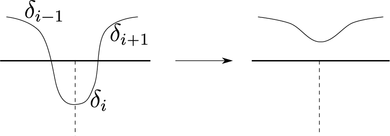
Figure 3 The bold edge is an edge of $\mathcal {T}$
and the dotted edge is an edge of
$\mathcal {T}$
and the dotted edge is an edge of $\mathcal {T}'$
that is not an edge of
$\mathcal {T}'$
that is not an edge of $\mathcal {T}$
.
$\mathcal {T}$
.
Repeating this reduction, we obtain a $\mathcal {T}$
-taut curve
$\mathcal {T}$
-taut curve $\bar {\gamma }$
homotopic to
$\bar {\gamma }$
homotopic to $\gamma $
. Let
$\gamma $
. Let $\bar {\gamma }_1,\ldots , \bar {\gamma }_m$
be its subcurves with respect to
$\bar {\gamma }_1,\ldots , \bar {\gamma }_m$
be its subcurves with respect to $\mathcal {T}$
, and
$\mathcal {T}$
, and $\bar {\gamma }_i$
be properly embedded into a band
$\bar {\gamma }_i$
be properly embedded into a band $(\bar {t}_i;\bar {e}_{i,1},\bar {e}_{i,2})$
. Since taut curves are unique in the homotopy class up to combinatorial equivalence, after reordering indices, we have
$(\bar {t}_i;\bar {e}_{i,1},\bar {e}_{i,2})$
. Since taut curves are unique in the homotopy class up to combinatorial equivalence, after reordering indices, we have $k=m$
and
$k=m$
and $(\bar {t}_i;\bar {e}_{i,1},\bar {e}_{i,2})=(t_i;e_{i,1},e_{i,2})$
. Then
$(\bar {t}_i;\bar {e}_{i,1},\bar {e}_{i,2})=(t_i;e_{i,1},e_{i,2})$
. Then $k=m \le l \le k'$
. The equality condition immediately follows from the constructions of
$k=m \le l \le k'$
. The equality condition immediately follows from the constructions of $\delta _i$
and
$\delta _i$
and $\bar {\gamma }_i$
.
$\bar {\gamma }_i$
.
3 Directed graphs and topological entropy of graph maps
A directed graph will be used throughout this article to understand the dynamics of branched coverings. In this section, we review basic notions of directed graphs and prove properties that we need in subsequent sections.
Let G be a finite directed graph. A path is a sequence of edges $(e_1, e_2, \ldots , e_n)$
such that the terminal vertex of
$(e_1, e_2, \ldots , e_n)$
such that the terminal vertex of $e_i$
is equal to the initial vertex of
$e_i$
is equal to the initial vertex of $e_{i+1}$
for every
$e_{i+1}$
for every $i\in [1,n-1]_{\mathbb {Z}}$
. The length of path is the number of edges in the sequence. The initial vertex of
$i\in [1,n-1]_{\mathbb {Z}}$
. The length of path is the number of edges in the sequence. The initial vertex of $e_1$
is the initial vertex of the path and the terminal vertex of
$e_1$
is the initial vertex of the path and the terminal vertex of $e_n$
is the terminal vertex of the path. If the initial and terminal vertices of a path p are v and w, then we call p a path from v to w. Let p and
$e_n$
is the terminal vertex of the path. If the initial and terminal vertices of a path p are v and w, then we call p a path from v to w. Let p and $p'$
be paths of length n and
$p'$
be paths of length n and $n'$
with
$n'$
with $n'>n$
. If the first n subsequence of edges of
$n'>n$
. If the first n subsequence of edges of $p'$
is equal to the sequence of edges of p, we say that
$p'$
is equal to the sequence of edges of p, we say that $p'$
is an extension of p and p is the first n-restriction of
$p'$
is an extension of p and p is the first n-restriction of $p'$
.
$p'$
.
A cycle is a path whose initial and terminal vertices coincide. A vertex is periodic if it is contained in a cycle and preperiodic if it is not periodic but there is a path from the vertex to a periodic vertex. For a subset $W \subset \operatorname{Vert}(G)$
, the subgraph generated by W is the subgraph of G consisting of W and edges connecting vertices in W.
$W \subset \operatorname{Vert}(G)$
, the subgraph generated by W is the subgraph of G consisting of W and edges connecting vertices in W.
Definition 3.1. (Recurrent paths)
For a periodic vertex $v\in \operatorname{Vert}(G)$
, a path p from v is recurrent if there exists a path from the terminal vertex w of p to v, that is, v and w are contained in one cycle. We also consider a periodic vertex as a recurrent path of length
$v\in \operatorname{Vert}(G)$
, a path p from v is recurrent if there exists a path from the terminal vertex w of p to v, that is, v and w are contained in one cycle. We also consider a periodic vertex as a recurrent path of length $0$
.
$0$
.
Definition 3.2. (Ideals)
Let G be a directed graph. A subset $X \subset \operatorname{Vert}(G)$
is an ideal if the following condition holds: for every
$X \subset \operatorname{Vert}(G)$
is an ideal if the following condition holds: for every $v\in X$
, if there is a path from v to w for some
$v\in X$
, if there is a path from v to w for some $w\in \operatorname{Vert}(G)$
, then
$w\in \operatorname{Vert}(G)$
, then $w\in X$
.
$w\in X$
.
For $v \in \operatorname{Vert}(G)$
, the ideal generated by v, denoted by
$v \in \operatorname{Vert}(G)$
, the ideal generated by v, denoted by $\langle v\rangle $
, is the collection of vertices
$\langle v\rangle $
, is the collection of vertices $w\in \operatorname{Vert}(G)$
where there is a path from v to w.
$w\in \operatorname{Vert}(G)$
where there is a path from v to w.
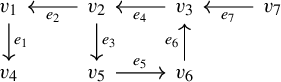
Example 3.3. Assume we have a directed graph as
Vertices $v_1$
and
$v_1$
and $v_4$
are neither periodic or preperiodic;
$v_4$
are neither periodic or preperiodic; $v_2,v_3,v_5,$
and
$v_2,v_3,v_5,$
and $v_6$
are periodic;
$v_6$
are periodic; $v_7$
is preperiodic. Starting from
$v_7$
is preperiodic. Starting from $v_3$
, the paths
$v_3$
, the paths $(e_4,e_3,e_5)$
and
$(e_4,e_3,e_5)$
and $(e_4,e_3,e_5,e_6,e_4,e_3)$
are recurrent, but the paths
$(e_4,e_3,e_5,e_6,e_4,e_3)$
are recurrent, but the paths $(e_4,e_2,e_1)$
and
$(e_4,e_2,e_1)$
and $(e_4,e_3,e_5,e_6,e_4,e_2)$
are not recurrent. There are only four ideals:
$(e_4,e_3,e_5,e_6,e_4,e_2)$
are not recurrent. There are only four ideals: $\{v_4\}, \{v_1,v_4\}, \{v_1,v_2,v_3,v_4,v_5,v_6\},$
and
$\{v_4\}, \{v_1,v_4\}, \{v_1,v_2,v_3,v_4,v_5,v_6\},$
and $\operatorname{Vert}(G)$
.
$\operatorname{Vert}(G)$
.
3.1 Adjacency matrices
Let G be a finite directed graph and $\operatorname{Vert}(G)\kern1.2pt{=}\kern1.2pt\{v_1, v_2,\ldots ,v_n\}\kern-0.5pt$
. The adjacency matrix A of G is defined by
$\operatorname{Vert}(G)\kern1.2pt{=}\kern1.2pt\{v_1, v_2,\ldots ,v_n\}\kern-0.5pt$
. The adjacency matrix A of G is defined by
 $$ \begin{align*} A_{ij}=\textrm{the number of edges from } v_i\textrm{ to }v_j, \end{align*} $$
where the $A_{ij}$
is the entry of the ith row and jth column of A. The adjacency matrix depends on the choice of indices of
$A_{ij}$
is the entry of the ith row and jth column of A. The adjacency matrix depends on the choice of indices of $v_i$
, and matrices defined by different choices of indices differ by conjugations by permutation matrices. In particular, if the index satisfies
$v_i$
, and matrices defined by different choices of indices differ by conjugations by permutation matrices. In particular, if the index satisfies $i<j$
only when there exists a path from
$i<j$
only when there exists a path from $v_i$
to
$v_i$
to $v_j$
, then the adjacency matrix is an upper triangular block matrix.
$v_j$
, then the adjacency matrix is an upper triangular block matrix.
 $$ \begin{align} A= \left( \begin{array}{ccccc} A_1 & * & \dots & * & *\\ 0 & A_2 & \dots & * & *\\ \vdots & \vdots & \ddots& \vdots & \vdots\\ 0& 0 & \dots & A_{k-1} & *\\ 0& 0 & \dots & 0 & A_k \end{array} \right), \end{align} $$
where $A_i$
is irreducible or a
$A_i$
is irreducible or a $0$
matrix. A non-negative
$0$
matrix. A non-negative $m \times m$
square matrix M is irreducible if for every
$m \times m$
square matrix M is irreducible if for every $1 \le i,j \le m$
, there exists
$1 \le i,j \le m$
, there exists $k\ge 1$
such that
$k\ge 1$
such that $(M^k)_{ij}>0$
. An irreducible non-negative matrix M has a simple eigenvalue, called the Perron–Frobenius eigenvalue, which is a positive real number and equal to the spectral radius of M. The spectral radius of A is equal to the maximum of Perron–Frobenius eigenvalues of the irreducible
$(M^k)_{ij}>0$
. An irreducible non-negative matrix M has a simple eigenvalue, called the Perron–Frobenius eigenvalue, which is a positive real number and equal to the spectral radius of M. The spectral radius of A is equal to the maximum of Perron–Frobenius eigenvalues of the irreducible $A_i$
. See [Reference Berman and PlemmonsBP94, Ch. 2].
$A_i$
. See [Reference Berman and PlemmonsBP94, Ch. 2].
3.1.1 Asymptotic growth of entries of
$A^n$

Let B be a non-negative irreducible matrix and denote by v and $w^T$
the right and the left eigenvectors of B which are normalized by
$w^T$
the right and the left eigenvectors of B which are normalized by $w^T v=1$
. By the Perron–Frobenius theorem, for the Perron–Frobenius eigenvalue
$w^T v=1$
. By the Perron–Frobenius theorem, for the Perron–Frobenius eigenvalue $\rho $
of B, we have
$\rho $
of B, we have
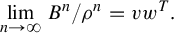 $$ \begin{align*} \lim_{n\to \infty} B^n/\rho^n=v w^T. \end{align*} $$
Hence, the $(i,j)$
entry of
$(i,j)$
entry of $B^n$
is asymptotic to
$B^n$
is asymptotic to $\rho ^n\cdot v_i \cdot w_j$
. This implies the following proposition. The proof is left to the reader.
$\rho ^n\cdot v_i \cdot w_j$
. This implies the following proposition. The proof is left to the reader.
Proposition 3.4. Let A be an $N\times N$
non-negative upper triangular block matrix such that
$N\times N$
non-negative upper triangular block matrix such that $A_1,\ldots A_k$
are blocks on the diagonal like equation (UTB-form). Let
$A_1,\ldots A_k$
are blocks on the diagonal like equation (UTB-form). Let $A_i$
be an
$A_i$
be an $N_i \times N_i$
matrix so that
$N_i \times N_i$
matrix so that $N=\sum _{i=1}^k N_i$
. For
$N=\sum _{i=1}^k N_i$
. For $i\in \{1,\ldots ,N\}$
, let
$i\in \{1,\ldots ,N\}$
, let $l_i \in [1,k]_{\mathbb {Z}}$
such that
$l_i \in [1,k]_{\mathbb {Z}}$
such that $A_{l_i}$
contains the
$A_{l_i}$
contains the $(i,i)$
-entry of A. Let
$(i,i)$
-entry of A. Let $R_{n,i}$
(respectively
$R_{n,i}$
(respectively $C_{n,i}$
) be the ith row (respectively column) sum of
$C_{n,i}$
) be the ith row (respectively column) sum of $A^n$
, that is, the sum of the entries in the ith row (respectively column) of
$A^n$
, that is, the sum of the entries in the ith row (respectively column) of $A^n$
. Then
$A^n$
. Then
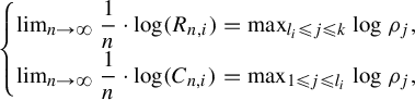 $$ \begin{align*} \begin{cases} \lim_{n\to \infty} \dfrac{1}{n} \cdot \log (R_{n,i})=\max_{l_i \le j \le k} \log \rho_j,\\[4pt] \lim_{n\to \infty} \dfrac{1}{n} \cdot \log (C_{n,i})=\max_{1 \le j \le l_i} \log \rho_j, \end{cases} \end{align*} $$
where $\rho _j$
is the spectral radius of
$\rho _j$
is the spectral radius of $A_j$
.
$A_j$
.
3.2 The growth rate of the number of paths
3.2.1 Polynomial and exponential growth rate
Suppose we have a sequence $\{a_n~|~a_n \in \mathbb {R}_{> 0},~n\ge 1\}$
. We consider sequences which are uniformly bounded or diverge to infinity when n tends to infinity. We say that the sequence has exponential growth, or grows exponentially fast, if there exists
$\{a_n~|~a_n \in \mathbb {R}_{> 0},~n\ge 1\}$
. We consider sequences which are uniformly bounded or diverge to infinity when n tends to infinity. We say that the sequence has exponential growth, or grows exponentially fast, if there exists $C>D>1$
such that for any sufficiently large
$C>D>1$
such that for any sufficiently large $n>0$
, we have
$n>0$
, we have
 $$ \begin{align*} D<{|}\!\log a_n|<C, \end{align*} $$
and the sequence has polynomial growth of degree d, or grows polynomially fast with degree d, for a non-negative integer d if there exists $C>D>0$
such that for any sufficiently large
$C>D>0$
such that for any sufficiently large $n>0$
, we have
$n>0$
, we have
 $$ \begin{align*} D\cdot n^d < a_n < C \cdot n^d. \end{align*} $$
Lemma 3.5. Suppose $\{a_n~|~n\ge 1,~a_n\ge 0 \}$
is a non-decreasing sequence. If there exist
$\{a_n~|~n\ge 1,~a_n\ge 0 \}$
is a non-decreasing sequence. If there exist $k,l,m>0$
such that
$k,l,m>0$
such that $a_{k\cdot n+l}\ge m \cdot n^d$
(respectively
$a_{k\cdot n+l}\ge m \cdot n^d$
(respectively $a_{k\cdot n+l}\le m \cdot n^d$
) for every
$a_{k\cdot n+l}\le m \cdot n^d$
) for every $n>0$
, then there exists
$n>0$
, then there exists $C>0$
such that
$C>0$
such that $a_n>C\cdot n^d$
(respectively
$a_n>C\cdot n^d$
(respectively $a_n<C\cdot n^d$
) for any sufficiently large n.
$a_n<C\cdot n^d$
) for any sufficiently large n.
Proof. Since the sequence $\{a_n\}$
is non-decreasing, we have
$\{a_n\}$
is non-decreasing, we have $a_{(k+1)\cdot n}\ge m \cdot n^d$
for any
$a_{(k+1)\cdot n}\ge m \cdot n^d$
for any $n>l/k$
. Then, for any sufficiently large
$n>l/k$
. Then, for any sufficiently large $n>0$
, we have
$n>0$
, we have
 $$ \begin{align*} a_n \ge a_{(k+1)\cdot\lfloor {n}/({k+1}) \rfloor}\ge m\cdot {\bigg\lfloor\frac{n}{k+1}\bigg\rfloor}^d>\frac{m}{(k+2)^d} \cdot n^d, \end{align*} $$
where $\lfloor x \rfloor $
means the largest integer less than or equal to x. The same argument also works for the inverse direction.
$\lfloor x \rfloor $
means the largest integer less than or equal to x. The same argument also works for the inverse direction.
Let G be a directed graph. Two paths in G are different if their sequences of edges are different. Let $P(v,n)$
be the number of different paths of length exactly n starting from v. The following criterion on the growth rate of
$P(v,n)$
be the number of different paths of length exactly n starting from v. The following criterion on the growth rate of $P(v,n)$
is well known. See [Reference SidkiSid00, Reference UfnarovskiĭUfn82]. We restate the criterion with a slight improvement for the case of polynomial growth.
$P(v,n)$
is well known. See [Reference SidkiSid00, Reference UfnarovskiĭUfn82]. We restate the criterion with a slight improvement for the case of polynomial growth.
Theorem 3.6. Let G be a directed graph and $v \in \operatorname{Vert}(G)$
.
$v \in \operatorname{Vert}(G)$
.
-
(1) If there exist two different cycles passing through v, then
$P(v,n)$
has exponential growth. -
(2) If there exists
$w\in \operatorname{Vert}(G)$
such that there are two different cycles starting from w and a path from v to w, then
$P(v,n)$
has exponential growth. -
(3) If v does not satisfy item (1) or (2), then
$P(v,n)$
has polynomial growth. Moreover, if the maximum number of (disjoint) cycles that a path from v can intersect is
$d+1$
, then the degree of the polynomial growth of
$P(v,n)$
is d. When the maximum number of cycles is zero, then
$P(v,n)=0$
for every sufficiently large n and we define the degree of polynomial growth to be
$-1$
.


Proof. The number of paths of length $\le n$
is counted in [Reference UfnarovskiĭUfn82] and we slightly modify it. If two cycles of lengths p and q pass through v, then there are at least
$\le n$
is counted in [Reference UfnarovskiĭUfn82] and we slightly modify it. If two cycles of lengths p and q pass through v, then there are at least $2^n$
paths of length
$2^n$
paths of length $npq$
starting from v. Let M be the maximal number of outgoing edges from one vertex in G. Then the number of paths with length n is less than
$npq$
starting from v. Let M be the maximal number of outgoing edges from one vertex in G. Then the number of paths with length n is less than $M^n$
. This proves items (1) and (2) is immediate from item
$M^n$
. This proves items (1) and (2) is immediate from item $(1)$
.
$(1)$
.
Assume that v does not satisfy item (1) or (2). Let $W=\langle v\rangle $
be the ideal generated by v. There exist totally ordered finite subsets
$W=\langle v\rangle $
be the ideal generated by v. There exist totally ordered finite subsets $W_1,\ldots W_k$
such that
$W_1,\ldots W_k$
such that $v \in W_i$
for each i and
$v \in W_i$
for each i and $W=\bigcup _{i=1}^k W_i$
. More precisely, we think of a directed graph H obtained by collapsing each cycle in G to a vertex. Since v does not satisfy item (1) or (2), the graph H does not have any cycle. Let
$W=\bigcup _{i=1}^k W_i$
. More precisely, we think of a directed graph H obtained by collapsing each cycle in G to a vertex. Since v does not satisfy item (1) or (2), the graph H does not have any cycle. Let $v'$
be the vertex of H corresponding to v. Then
$v'$
be the vertex of H corresponding to v. Then $v'$
is the only minimal element of
$v'$
is the only minimal element of $\operatorname{Vert}(H)$
. Let
$\operatorname{Vert}(H)$
. Let $w_1,w_2,\ldots ,w_m$
be the maximal elements of
$w_1,w_2,\ldots ,w_m$
be the maximal elements of $\operatorname{Vert}(H)$
. Choose any
$\operatorname{Vert}(H)$
. Choose any $w\in \operatorname{Vert}(W)$
.
$w\in \operatorname{Vert}(W)$
.
Then the subgraph $G_i$
generated by
$G_i$
generated by $W_i$
is isomorphic to the graph in Figure 4. Since every path from v is supported in some
$W_i$
is isomorphic to the graph in Figure 4. Since every path from v is supported in some $G_i$
, it suffices to show item
$G_i$
, it suffices to show item $(3)$
when G is the graph of the type shown in Figure 4.
$(3)$
when G is the graph of the type shown in Figure 4.
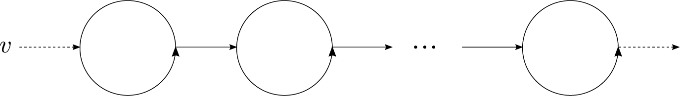
Figure 4 A graph with polynomial growth rate of $P(v,n)$
. Any arrow indicates paths, any dotted arrow means it may not exist but if exists it indicates a path, and any circle indicates a cycle. In each cycle, the incoming vertex and the outgoing vertex could be the same.
$P(v,n)$
. Any arrow indicates paths, any dotted arrow means it may not exist but if exists it indicates a path, and any circle indicates a cycle. In each cycle, the incoming vertex and the outgoing vertex could be the same.
Assume G is a graph of the type in Figure 4. Let it have $d+1$
cycles of lengths
$d+1$
cycles of lengths $p_1,p_2,\ldots , p_{d+1}$
. Let
$p_1,p_2,\ldots , p_{d+1}$
. Let $p_M$
and
$p_M$
and $p_m$
be the maximum and minimum of
$p_m$
be the maximum and minimum of $\{p_1,\ldots , p_d\}$
, and K and L be the number of vertices and edges of G, respectively. Let
$\{p_1,\ldots , p_d\}$
, and K and L be the number of vertices and edges of G, respectively. Let $X(n)$
be the set of d-tuples
$X(n)$
be the set of d-tuples $(n_1,\ldots ,n_d)$
of non-negative integers satisfying
$(n_1,\ldots ,n_d)$
of non-negative integers satisfying $n_1 + \cdots +n_d \le n$
. The set
$n_1 + \cdots +n_d \le n$
. The set $X(n)$
has
$X(n)$
has $\binom {n+d}{d}$
elements.
$\binom {n+d}{d}$
elements.
Claim. For any $n\ge 1$
,
$n\ge 1$
, $P(v,p_m\cdot n)/K \le \binom {n+d}{d} \le P(v,p_M \cdot n +L)$
.
$P(v,p_m\cdot n)/K \le \binom {n+d}{d} \le P(v,p_M \cdot n +L)$
.
Proof of claim
For any n, we define an injective map from $X(n)$
to the set of paths from v of length
$X(n)$
to the set of paths from v of length $p_M\cdot n+L$
as follows. For any
$p_M\cdot n+L$
as follows. For any $(n_1,\ldots ,n_d)\in X(n)$
, we have a path from v which goes around the ith cycle
$(n_1,\ldots ,n_d)\in X(n)$
, we have a path from v which goes around the ith cycle $n_i$
times for
$n_i$
times for $i \le d$
. The path has length not greater than
$i \le d$
. The path has length not greater than $p_M\cdot n + L$
. There is a unique extension of the path which: (1) does not further go around the first d cycles, that is, the additional rotations occur only in the last cycle and (2) has length exactly equal to
$p_M\cdot n + L$
. There is a unique extension of the path which: (1) does not further go around the first d cycles, that is, the additional rotations occur only in the last cycle and (2) has length exactly equal to $p_M\cdot n + L$
. We assign the extended path to the element
$p_M\cdot n + L$
. We assign the extended path to the element $(n_1,\ldots ,n_d)\in X(n)$
. Hence, we have
$(n_1,\ldots ,n_d)\in X(n)$
. Hence, we have $\binom {n+d}{d} \le P(v,p_M\cdot n+L)$
.
$\binom {n+d}{d} \le P(v,p_M\cdot n+L)$
.
Similarly, we define another map from the set of paths of length $p_m\cdot n$
to
$p_m\cdot n$
to $X(n)$
by assigning the numbers of times that each path goes around the first d cycles. Suppose that two such paths
$X(n)$
by assigning the numbers of times that each path goes around the first d cycles. Suppose that two such paths $p_1$
and
$p_1$
and $p_2$
have the same image in
$p_2$
have the same image in $X(n)$
. Since
$X(n)$
. Since $p_1$
and
$p_1$
and $p_2$
start from the same vertex v and have the same length, their terminal vertex are the same if and only if
$p_2$
start from the same vertex v and have the same length, their terminal vertex are the same if and only if $p_1$
and
$p_1$
and $p_2$
are the same. It follows that the number of preimages of the map is less than K.
$p_2$
are the same. It follows that the number of preimages of the map is less than K.
As $\binom {n+d}{d}$
is a degree d polynomial in n, it follows from Lemma 3.5 that the
$\binom {n+d}{d}$
is a degree d polynomial in n, it follows from Lemma 3.5 that the $P(v,n)$
has polynomial growth of degree d as a sequence in n.
$P(v,n)$
has polynomial growth of degree d as a sequence in n.
The polynomial growth rate of $P(v,n)$
implies the recurrent extension is unique.
$P(v,n)$
implies the recurrent extension is unique.
Proposition 3.7. (Extension of recurrent paths)
Let G be a directed graph and $v\in \operatorname{Vert}(G)$
. Let
$v\in \operatorname{Vert}(G)$
. Let $\gamma $
be a path from v of length
$\gamma $
be a path from v of length $m>0$
. If
$m>0$
. If $\gamma $
is recurrent, then for any
$\gamma $
is recurrent, then for any $n>m$
,
$n>m$
, $\gamma $
has at least one extension to a recurrent path of length n. Moreover, if
$\gamma $
has at least one extension to a recurrent path of length n. Moreover, if $P(v,n)$
grows polynomially fast as n tends to
$P(v,n)$
grows polynomially fast as n tends to $\infty $
, then the extension is unique.
$\infty $
, then the extension is unique.
Proof. Since $\gamma $
is recurrent, the initial and the terminal points of
$\gamma $
is recurrent, the initial and the terminal points of $\gamma $
belong to one cycle C of G. Then we can extend
$\gamma $
belong to one cycle C of G. Then we can extend $\gamma $
by repeatedly traveling along C. If
$\gamma $
by repeatedly traveling along C. If $P(v,n)$
grows polynomially fast, then C is the only cycle that passes through v. Hence, traveling along C is the only way to extend
$P(v,n)$
grows polynomially fast, then C is the only cycle that passes through v. Hence, traveling along C is the only way to extend $\gamma $
.
$\gamma $
.
3.3 Graph maps with zero topological entropy
Let G be a finite graph and $\operatorname{Vert}(G)$
be its vertex set. A continuous map
$\operatorname{Vert}(G)$
be its vertex set. A continuous map $f:G \to G$
is Markov if
$f:G \to G$
is Markov if $f(\operatorname{Vert}(G)) \subset \operatorname{Vert}(G)$
and f is a homeomorphism or constant on each component of
$f(\operatorname{Vert}(G)) \subset \operatorname{Vert}(G)$
and f is a homeomorphism or constant on each component of $G \setminus f^{-1}(\operatorname{Vert}(G))$
. Then the edges form a Markov partition of f. Denote by
$G \setminus f^{-1}(\operatorname{Vert}(G))$
. Then the edges form a Markov partition of f. Denote by $e_1,e_2,\ldots $
the edges of G. Note that every edge is mapped to a union of edges. The adjacency matrix
$e_1,e_2,\ldots $
the edges of G. Note that every edge is mapped to a union of edges. The adjacency matrix $A_f$
of
$A_f$
of $f:G \to G$
is defined in such a way that
$f:G \to G$
is defined in such a way that $f(e_i)$
covers
$f(e_i)$
covers $e_j$
as many as the
$e_j$
as many as the $(i,\,j)$
entry of
$(i,\,j)$
entry of $A_f$
. Under a suitable choice of indexing
$A_f$
. Under a suitable choice of indexing $e_i$
terms, we may assume that
$e_i$
terms, we may assume that $A_f$
is an upper triangular block matrix. Let
$A_f$
is an upper triangular block matrix. Let $A_1,\ldots A_k$
be the block matrices on the diagonal as in equation (UTB-form).
$A_1,\ldots A_k$
be the block matrices on the diagonal as in equation (UTB-form).
The spectral radius $\unicode{x3bb} $
of
$\unicode{x3bb} $
of $A_f$
is either equal to zero if every
$A_f$
is either equal to zero if every $A_i$
is zero or equal to the maximum of Perron–Frobenius eigenvalues of the irreducible
$A_i$
is zero or equal to the maximum of Perron–Frobenius eigenvalues of the irreducible $A_i$
terms. The topological entropy
$A_i$
terms. The topological entropy $h_{\textrm {top}}(f)$
of f is equal to zero if
$h_{\textrm {top}}(f)$
of f is equal to zero if $\unicode{x3bb} =0$
or equal to
$\unicode{x3bb} =0$
or equal to $\log (\unicode{x3bb} )$
if
$\log (\unicode{x3bb} )$
if $\unicode{x3bb}>0$
. The relationship between the topological entropy and the Perron–Frobenius eigenvalue follows from [Reference Misiurewicz and SzlenkMS80].
$\unicode{x3bb}>0$
. The relationship between the topological entropy and the Perron–Frobenius eigenvalue follows from [Reference Misiurewicz and SzlenkMS80].
There is a directed graph $\mathcal {D}_f$
such that
$\mathcal {D}_f$
such that $\operatorname{Vert}(\mathcal {D}_f) = \operatorname {\textrm {Edge}}(G)$
and the directed edges are defined as follows: for
$\operatorname{Vert}(\mathcal {D}_f) = \operatorname {\textrm {Edge}}(G)$
and the directed edges are defined as follows: for $e_i,e_j\in \operatorname {\textrm {Edge}}(G)$
, if
$e_i,e_j\in \operatorname {\textrm {Edge}}(G)$
, if $f(e_i)$
covers
$f(e_i)$
covers $e_j$
exactly k times, then we draw k directed edges of
$e_j$
exactly k times, then we draw k directed edges of $\mathcal {D}_f$
from
$\mathcal {D}_f$
from $e_i$
to
$e_i$
to $e_j$
. Then
$e_j$
. Then $A_f$
is equal to the adjacency matrix of
$A_f$
is equal to the adjacency matrix of $\mathcal {D}_f$
. We refer to
$\mathcal {D}_f$
. We refer to $\mathcal {D}_f$
as the directed graph of the Markov map
$\mathcal {D}_f$
as the directed graph of the Markov map $f:G\to G$
.
$f:G\to G$
.
The following lemma is elementary, but we prove it for the sake of self-containedness.
Lemma 3.8. Let M be an irreducible non-negative integer matrix and $\unicode{x3bb} (M)$
be its Perron–Frobenius eigenvalue. Then
$\unicode{x3bb} (M)$
be its Perron–Frobenius eigenvalue. Then $\unicode{x3bb} (M) \ge 1$
and the equality holds if and only if M is a permutation matrix.
$\unicode{x3bb} (M) \ge 1$
and the equality holds if and only if M is a permutation matrix.
Proof. Because the characteristic polynomial of M is a monic polynomial with integer coefficients, the absolute value of the product of eigenvalues is a positive integer. Hence, the spectral radius $\unicode{x3bb} (M)$
is at least one. If M is a permutation matrix, then trivially
$\unicode{x3bb} (M)$
is at least one. If M is a permutation matrix, then trivially $\unicode{x3bb} (M)=1$
. Assume
$\unicode{x3bb} (M)=1$
. Assume $\unicode{x3bb} (M)=1$
. Let H be a directed graph whose adjacency matrix is M. Since M is irreducible, for any pair
$\unicode{x3bb} (M)=1$
. Let H be a directed graph whose adjacency matrix is M. Since M is irreducible, for any pair $(v,w)$
of vertices of H, there exists a path
$(v,w)$
of vertices of H, there exists a path $p_1$
from v to w and a path
$p_1$
from v to w and a path $p_2$
from w to v. If there exists a vertex
$p_2$
from w to v. If there exists a vertex $x\neq v,w$
through which both paths
$x\neq v,w$
through which both paths $p_1$
and
$p_1$
and $p_2$
pass, there are two different cycles passing through x. By Theorem 3.6, the number of length-n paths
$p_2$
pass, there are two different cycles passing through x. By Theorem 3.6, the number of length-n paths $P(x,n)$
grows exponentially fast. Since
$P(x,n)$
grows exponentially fast. Since $P(x,n)$
is the sum of entries in the row of
$P(x,n)$
is the sum of entries in the row of $M^n$
corresponding to the vertex v, it follows that
$M^n$
corresponding to the vertex v, it follows that $\unicode{x3bb} (M)>1$
. So
$\unicode{x3bb} (M)>1$
. So $p_1$
and
$p_1$
and $p_2$
form a cycle which passes through vertices exactly once. If there is a vertex x that is not contained in this cycle, then there is a path from x to v and a path from v to x. Then two different cycles pass through v so
$p_2$
form a cycle which passes through vertices exactly once. If there is a vertex x that is not contained in this cycle, then there is a path from x to v and a path from v to x. Then two different cycles pass through v so $P(v,n)$
grows exponentially fast and
$P(v,n)$
grows exponentially fast and $\unicode{x3bb} (M)>1$
. Hence, H is a cycle passing through every vertex exactly once, and M is a permutation matrix.
$\unicode{x3bb} (M)>1$
. Hence, H is a cycle passing through every vertex exactly once, and M is a permutation matrix.
Proposition 3.9. Let $f:G \to G$
be a Markov map. Then the following are equivalent.
$f:G \to G$
be a Markov map. Then the following are equivalent.
-
(1) The topological entropy
$h_{\textrm {top}}(f)$
is zero. -
(2) Every irreducible block
$A_i$
of the upper-triangular block form of the adjacency matrix
$A_f$
is a permutation matrix. -
(3) The directed graph
$\mathcal {D}_f$
of the adjacency matrix
$A_f$
has disjoint cycles, that is, every pair of different cycles has disjoint vertices. -
(4) There exists a positive integer d such that
$({A_f}^n)_{ij}=O(n^d)$
for all
$i,\,j$
.


Proof. $(3) \Leftrightarrow (2)\Rightarrow (1)$
is trivial and
$(3) \Leftrightarrow (2)\Rightarrow (1)$
is trivial and $(4) \Leftrightarrow (3)$
is immediate from Theorem 3.6. Assume
$(4) \Leftrightarrow (3)$
is immediate from Theorem 3.6. Assume $h_{\textrm {top}}(f)=0$
. Then the Perron–Frobenius eigenvalue of every irreducible block
$h_{\textrm {top}}(f)=0$
. Then the Perron–Frobenius eigenvalue of every irreducible block $A_i$
of the adjacency matrix
$A_i$
of the adjacency matrix $A_f$
is one.
$A_f$
is one. $(1) \Rightarrow (2)$
follows from Lemma 3.8.
$(1) \Rightarrow (2)$
follows from Lemma 3.8.
4 Finite subdivision rules
A finite subdivision rule $\mathcal {R}$
consists of the following:
$\mathcal {R}$
consists of the following:
-
(1) a subdivision complex
$S_{\mathcal {R}}$
which is a two-dimensional finite CW-complex such that the underlying space is the union of its closed
$2$
-cells, that is, every
$0$
- or
$1$
-cell is on the boundary of a
$2$
-cell; -
(2) a subdivision
$\mathcal {R}(S_{\mathcal {R}})$
of
$S_{\mathcal {R}}$
that is a CW-complex for which every open cell is contained in an open cell of
$S_{\mathcal {R}}$
; and -
(3) a subdivision map
$f:\mathcal {R}(S_{\mathcal {R}}) \rightarrow S_{\mathcal {R}}$
which is continuous and cell-wise homeomorphic, that is, its restriction to each open cell is a homeomorphism onto an open cell.


We say that $\mathcal {R}$
is orientation preserving if every
$\mathcal {R}$
is orientation preserving if every $2$
-cell can be oriented in such a way that f preserves the orientation. Similarly,
$2$
-cell can be oriented in such a way that f preserves the orientation. Similarly, $\mathcal {R}$
is orientation reversing if f reverses the orientation on every cell. For any closed
$\mathcal {R}$
is orientation reversing if f reverses the orientation on every cell. For any closed $2$
-cell t of
$2$
-cell t of $S_{\mathcal {R}}$
, there exists a n-gon
$S_{\mathcal {R}}$
, there exists a n-gon $\textbf {t}$
and the characteristic map
$\textbf {t}$
and the characteristic map $\phi _t:\textbf {t} \to t$
is cell-wise homeomorphic. The CW-complex
$\phi _t:\textbf {t} \to t$
is cell-wise homeomorphic. The CW-complex $\textbf {t}$
is called the tile type of the closed
$\textbf {t}$
is called the tile type of the closed $2$
-cell t. Similarly, for a characteristic map of a
$2$
-cell t. Similarly, for a characteristic map of a $1$
-cell
$1$
-cell $\phi _e:\textbf {e} \to e$
,
$\phi _e:\textbf {e} \to e$
, $\textbf {e}$
is the edge type of a closed
$\textbf {e}$
is the edge type of a closed $1$
-cell e.
$1$
-cell e.
A two-dimensional CW-complex X is an $\mathcal {R}$
-complex if it is the union of its closed
$\mathcal {R}$
-complex if it is the union of its closed $2$
-cells and there is a continuous cell-wise homeomorphism
$2$
-cells and there is a continuous cell-wise homeomorphism $g:X \rightarrow S_{\mathcal {R}}$
. By pulling back the subdivision
$g:X \rightarrow S_{\mathcal {R}}$
. By pulling back the subdivision $\mathcal {R}^n(S_{\mathcal {R}})$
of
$\mathcal {R}^n(S_{\mathcal {R}})$
of $S_{\mathcal {R}}$
through g for each
$S_{\mathcal {R}}$
through g for each $n>0$
, we also have a subdivision
$n>0$
, we also have a subdivision $\mathcal {R}^n(X)$
of X and a cell-wise homeomorphism
$\mathcal {R}^n(X)$
of X and a cell-wise homeomorphism $f^{\circ n} \circ g:\mathcal {R}^n(X) \rightarrow S_{\mathcal {R}}$
. For example,
$f^{\circ n} \circ g:\mathcal {R}^n(X) \rightarrow S_{\mathcal {R}}$
. For example, $S_{\mathcal {R}}$
itself and any tile type
$S_{\mathcal {R}}$
itself and any tile type $\textbf {t}$
are
$\textbf {t}$
are $\mathcal {R}$
-complexes, so for any
$\mathcal {R}$
-complexes, so for any $n \in \mathbb {N}$
, their level-n subdivisions
$n \in \mathbb {N}$
, their level-n subdivisions $\mathcal {R}^n(S_{\mathcal {R}})$
and
$\mathcal {R}^n(S_{\mathcal {R}})$
and $\mathcal {R}^n(\textbf {t})$
are defined. For any edge type
$\mathcal {R}^n(\textbf {t})$
are defined. For any edge type $\textbf {e}$
, its level-n subdivision
$\textbf {e}$
, its level-n subdivision $\mathcal {R}^n(\textbf {e})$
is also similarly defined.
$\mathcal {R}^n(\textbf {e})$
is also similarly defined.
We call a closed $2$
-cell (respectively a closed
$2$
-cell (respectively a closed $1$
-cell, a
$1$
-cell, a $0$
-cell) a tile (respectively an edge, a vertex) of a two-dimensional complex. Every level-
$0$
-cell) a tile (respectively an edge, a vertex) of a two-dimensional complex. Every level- $0$
tile or edge of an
$0$
tile or edge of an $\mathcal {R}$
-complex is also an
$\mathcal {R}$
-complex is also an $\mathcal {R}$
-complex. See [Reference Cannon, Floyd and ParryCFP01] for more details on finite subdivision rules.
$\mathcal {R}$
-complex. See [Reference Cannon, Floyd and ParryCFP01] for more details on finite subdivision rules.
4.1 Notation
As we wrote in the previous paragraph, we use bold fonts for the domains of characteristic maps and normal fonts for the corresponding closed cells in the CW-complexes. For example, for a closed $2$
-cell t in a CW-complex X, we write
$2$
-cell t in a CW-complex X, we write $\phi _t:\textbf {t}\to t$
for the characteristic map. Thus,
$\phi _t:\textbf {t}\to t$
for the characteristic map. Thus, $\textbf {t}$
is always homeomorphic to the closed
$\textbf {t}$
is always homeomorphic to the closed $2$
-disk, but t may not be.
$2$
-disk, but t may not be.
4.2 Subdivision maps as post-critically finite branched coverings
Throughout this article, we assume $S_{\mathcal {R}}$
is homeomorphic to the
$S_{\mathcal {R}}$
is homeomorphic to the $2$
-sphere
$2$
-sphere $S^2$
. Considering
$S^2$
. Considering $\mathcal {R}(S_{\mathcal {R}})$
and
$\mathcal {R}(S_{\mathcal {R}})$
and $S_{\mathcal {R}}$
as different complexes on the same underlying
$S_{\mathcal {R}}$
as different complexes on the same underlying $2$
-sphere, we may think of the subdivision map
$2$
-sphere, we may think of the subdivision map $f:\mathcal {R}(S_{\mathcal {R}}) \rightarrow S_{\mathcal {R}}$
as a topological branched self-covering of
$f:\mathcal {R}(S_{\mathcal {R}}) \rightarrow S_{\mathcal {R}}$
as a topological branched self-covering of $S^2$
. Since the set of critical points
$S^2$
. Since the set of critical points $\Omega _f$
is a subset of the set of vertices of
$\Omega _f$
is a subset of the set of vertices of $\mathcal {R}(S_{\mathcal {R}})$
, f is post-critically finite.
$\mathcal {R}(S_{\mathcal {R}})$
, f is post-critically finite.
A set of marked points A of $\mathcal {R}$
is a subset of
$\mathcal {R}$
is a subset of $\operatorname{Vert}(S_{\mathcal {R}})$
with
$\operatorname{Vert}(S_{\mathcal {R}})$
with $P_f \cup f(A) \subset A$
. With a choice of a set of marked points A, the subdivision map can be considered as a marked post-critically finite branched covering
$P_f \cup f(A) \subset A$
. With a choice of a set of marked points A, the subdivision map can be considered as a marked post-critically finite branched covering ![]() .
.
4.3 Branched coverings represented as subdivision maps
If f is a subdivision map, then the $1$
-skeleton
$1$
-skeleton $S_{\mathcal {R}}^{(1)}$
is a graph such that: (1) it contains
$S_{\mathcal {R}}^{(1)}$
is a graph such that: (1) it contains $P_f$
; (2) it is connected; and (3) it is forward invariant under f. Conversely, if there is a graph satisfying the three conditions, then it defines a finite subdivision rule. Below is a list of some forward invariant graphs that are known to exist.
$P_f$
; (2) it is connected; and (3) it is forward invariant under f. Conversely, if there is a graph satisfying the three conditions, then it defines a finite subdivision rule. Below is a list of some forward invariant graphs that are known to exist.
-
• Spiders of polynomials [Reference Hubbard, Schleicher, Branner, Keen, Douady, Blanchard, Hubbard, Schleicher and DevaneyHS94].
-
• Hubbard trees that can be augmented to be invariant trees [Reference Shepelevtseva and TimorinST19].
-
• Jordan curves [Reference Bonk and MeyerBM17] and trees [Reference HlushchankaHlu17] of expanding Thurston maps.
-
• Tischler graphs of critically fixed rational maps [Reference HlushchankaHlu19, Reference Pilgrim and TanPT98].
-
• Jordan curves [Reference Gao, Haïssinsky, Meyer and ZengGHMZ18] and trees [Reference HlushchankaHlu17] of Sierpiński Carpet rational maps.
-
• Extended Newton graphs for post-critically finite Newton maps [Reference Lodge, Mikulich and SchleicherLMS21].
-
• A sufficiently large iterate
$f^n$
of any post-critically finite branched covering f without a Levy cycle is homotopic to a subdivision map [Reference Floyd, Parry and PilgrimFPP20]. Its 1-skeleton is invariant up to homotopy.

There are post-critically finite branched coverings whose any iterates cannot be represented as subdivision maps [Reference Floyd, Parry and PilgrimFPP20, §4].
4.4 Combinatorial properties of
$\mathcal {R}$
and Levy and Thurston obstructions

A finite subdivision rule $\mathcal {R}$
is edge separating if for every tile type
$\mathcal {R}$
is edge separating if for every tile type $\textbf {t}$
and pair of disjoint closed edges e and
$\textbf {t}$
and pair of disjoint closed edges e and $e'$
of
$e'$
of $\textbf {t}$
, there exists a positive integer n such that no subtile of
$\textbf {t}$
, there exists a positive integer n such that no subtile of $\textbf {t}$
in
$\textbf {t}$
in $\mathcal {R}^n(\textbf {t})$
contains both a subedge of e and a subedge of
$\mathcal {R}^n(\textbf {t})$
contains both a subedge of e and a subedge of $e'$
. Similarly,
$e'$
. Similarly, $\mathcal {R}$
is vertex separating if for every tile type
$\mathcal {R}$
is vertex separating if for every tile type $\textbf {t}$
and pair of vertices v and w of
$\textbf {t}$
and pair of vertices v and w of $\textbf {t}$
, there exists a positive integer n such that no subtile of
$\textbf {t}$
, there exists a positive integer n such that no subtile of $\textbf {t}$
in
$\textbf {t}$
in $\mathcal {R}^n(\textbf {t})$
contains both v and w. These two separating conditions are a part of the sufficient condition for a subdivision map not having a Levy cycle or a Thurston obstruction.
$\mathcal {R}^n(\textbf {t})$
contains both v and w. These two separating conditions are a part of the sufficient condition for a subdivision map not having a Levy cycle or a Thurston obstruction.
-
• If
$\mathcal {R}$
is vertex separating and edge separating, then f does not have a Levy cycle [Reference Floyd, Parry and PilgrimFPP18b, Proposition 5.1]. There is a finite subdivision rule which is neither edge separating nor vertex separating but does not have a Levy cycle, see Example 4.2. -
• If
$\mathcal {R}$
is vertex separating, edge separating, and conformal (we do not define this conformality in the article), then f does not have a Thurston obstruction [Reference Cannon, Floyd, Kenyon and ParryCFKP03]. There is an example [Reference Cannon, Floyd, Kenyon and ParryCFKP03, Example 4.6] of finite subdivision rule which is not conformal but does not have a Thurston obstruction, thus it is combinatorially equivalent to a rational map. See [Reference Cannon, Floyd, Kenyon and ParryCFKP03] for a definition of conformal finite subdivision rules.


Example 4.2. The finite subdivision rule R given in Figure 5 is [Reference Floyd, Parry and PilgrimFPP18b, Example 5.3]. Its CW-complex $\mathcal {S}_{\mathcal {R}}$
of the
$\mathcal {S}_{\mathcal {R}}$
of the $2$
-sphere consists of two square tiles. The edges of white and shaded tiles are glued to form a pillowcase. Since the shaded tile does not subdivide,
$2$
-sphere consists of two square tiles. The edges of white and shaded tiles are glued to form a pillowcase. Since the shaded tile does not subdivide, $\mathcal {R}$
is neither edge separating nor vertex separating. However, it easily follows from Theorem 6.21 that the subdivision map does not have a Levy cycle.
$\mathcal {R}$
is neither edge separating nor vertex separating. However, it easily follows from Theorem 6.21 that the subdivision map does not have a Levy cycle.
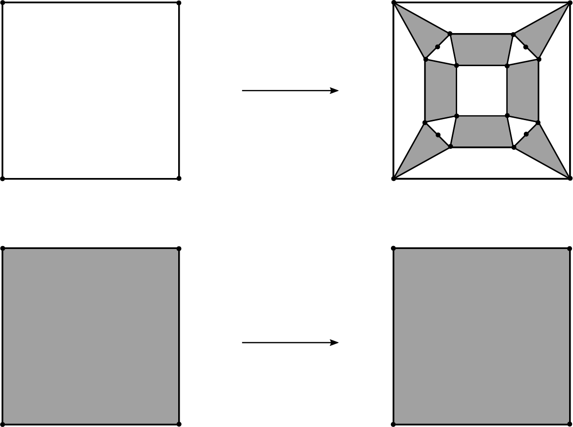
Figure 5 An example of expanding finite subdivision rule which is neither edge separating nor vertex separating.
4.5 Edges, bands, bones, and curves of subdivision complexes
For $n\ge 0$
, a level- n tile, edge, or band of
$n\ge 0$
, a level- n tile, edge, or band of $\mathcal {R}$
is a tile, edge, or band of
$\mathcal {R}$
is a tile, edge, or band of $\mathcal {R}^n(S_{\mathcal {R}})$
. See Definition 2.1 for definitions of bands and their bones. There is a bijection between level-
$\mathcal {R}^n(S_{\mathcal {R}})$
. See Definition 2.1 for definitions of bands and their bones. There is a bijection between level- $0$
tiles (respectively edge) and tile types (respectively edge types); a level-
$0$
tiles (respectively edge) and tile types (respectively edge types); a level- $0$
tile t is the image of the tile type
$0$
tile t is the image of the tile type $\textbf {t}$
under the characteristic map
$\textbf {t}$
under the characteristic map $\phi _t:\textbf {t}\to t$
.
$\phi _t:\textbf {t}\to t$
.
We will use superscripts to indicate the level of tiles, edges, etc. Since frequently considering level- $0$
objects, we sometimes omit the superscript
$0$
objects, we sometimes omit the superscript $^0$
for simplicity.
$^0$
for simplicity.
For $n>m$
, a level-n tile
$n>m$
, a level-n tile $t^n$
is a subtile of a level-m tile
$t^n$
is a subtile of a level-m tile $t^m$
if
$t^m$
if $t^{n} \subset t^{m}$
. Let
$t^{n} \subset t^{m}$
. Let $\textbf {t}$
be a tile type and t be the corresponding level-
$\textbf {t}$
be a tile type and t be the corresponding level- $0$
tile. A level-n tile
$0$
tile. A level-n tile $t^n$
is of type
$t^n$
is of type $\textbf {t}$
if
$\textbf {t}$
if $f^n(t^n)=t$
. Subedges and their types are similarly defined. A band type is a level-
$f^n(t^n)=t$
. Subedges and their types are similarly defined. A band type is a level- $0$
band. For a band type
$0$
band. For a band type $(t;e_1,e_2)$
, a level-n band
$(t;e_1,e_2)$
, a level-n band $(t^n;e_1^n,e_2^n)$
is of type
$(t^n;e_1^n,e_2^n)$
is of type $(t;e_1,e_2)$
if the
$(t;e_1,e_2)$
if the $f^n$
-image of its bone is the bone of
$f^n$
-image of its bone is the bone of $(t;e_1,e_2)$
(or, equivalently, if
$(t;e_1,e_2)$
(or, equivalently, if $t^n$
is of type
$t^n$
is of type $\textbf {t}$
and
$\textbf {t}$
and $e_i^n$
is of type
$e_i^n$
is of type $\textbf {e}_i$
for
$\textbf {e}_i$
for $i=1,2$
. For
$i=1,2$
. For $n>m$
, a level-n band
$n>m$
, a level-n band $(t^n;e_1^n,e_2^n)$
is a subband of a level-m band
$(t^n;e_1^n,e_2^n)$
is a subband of a level-m band $(t^m;e_1^m,e_2^m)$
if
$(t^m;e_1^m,e_2^m)$
if $t^n\subset t^m$
and
$t^n\subset t^m$
and $e_i^n \subset e_i^m$
for
$e_i^n \subset e_i^m$
for $i=1,2$
. If
$i=1,2$
. If $\deg (f)=d$
, there are
$\deg (f)=d$
, there are $d^n$
level-n tiles, edges, and bands of the same type.
$d^n$
level-n tiles, edges, and bands of the same type.
Definition 4.3. (Abbreviations for level-n bands and bones)
There are many level-n bands that are not subbands of level- $0$
bands. However, the only level-n bands that we consider are level-n subbands of level-
$0$
bands. However, the only level-n bands that we consider are level-n subbands of level- $0$
bands. Since these objects will be very frequently used, for the sake of simple notation, by a level-n band, we mean a level-n subband of a level-
$0$
bands. Since these objects will be very frequently used, for the sake of simple notation, by a level-n band, we mean a level-n subband of a level- $0$
band. Similarly, by a level-n bone, we mean the bone of a level-n subband of a level-
$0$
band. Similarly, by a level-n bone, we mean the bone of a level-n subband of a level- $0$
band.
$0$
band.
Definition 4.4. (Non-expanded level-n curves)
Let $\mathcal {R}$
be a finite subdivision rule. Let I be a closed interval
$\mathcal {R}$
be a finite subdivision rule. Let I be a closed interval $[k,l]$
,
$[k,l]$
, $(-\infty ,k]$
,
$(-\infty ,k]$
, $[k,\infty )$
, or
$[k,\infty )$
, or $(-\infty ,\infty )$
for
$(-\infty ,\infty )$
for $k<l\in \mathbb {Z}$
. For
$k<l\in \mathbb {Z}$
. For $n\ge 0$
, a curve
$n\ge 0$
, a curve $\gamma ^n:I\to \mathcal {R}^n(S_{\mathcal {R}})$
is a non-expanded level-n curve if
$\gamma ^n:I\to \mathcal {R}^n(S_{\mathcal {R}})$
is a non-expanded level-n curve if $\gamma ^n([i,i+1])$
is a level-n bone for every
$\gamma ^n([i,i+1])$
is a level-n bone for every $i\in \mathbb {Z}$
with
$i\in \mathbb {Z}$
with $[i,i+1]\subset I$
. A non-expanded level-n curve is recurrent if it consists of level-n bones that are recurrent. The recurrent bands and bones are defined in Definition 4.8.
$[i,i+1]\subset I$
. A non-expanded level-n curve is recurrent if it consists of level-n bones that are recurrent. The recurrent bands and bones are defined in Definition 4.8.
4.6 Two directed graphs defined from finite subdivision rules
4.6.1 Directed graphs of edge subdivisions
Let $\mathcal {E}$
be a directed graph such that
$\mathcal {E}$
be a directed graph such that $\operatorname{Vert}(\mathcal {E})$
is the same as the set of level-
$\operatorname{Vert}(\mathcal {E})$
is the same as the set of level- $0$
edges. To avoid confusion, we denote by
$0$
edges. To avoid confusion, we denote by $[e]$
the vertex of
$[e]$
the vertex of $\mathcal {E}$
corresponding to an edge e. A directed edge from
$\mathcal {E}$
corresponding to an edge e. A directed edge from $[e]$
to
$[e]$
to $[e']$
corresponds to a level-
$[e']$
corresponds to a level- $1$
subedge of e of type
$1$
subedge of e of type $\textbf {e}'$
. We call
$\textbf {e}'$
. We call $\mathcal {E}$
the directed graph of edge subdivision of
$\mathcal {E}$
the directed graph of edge subdivision of $\mathcal {R}$
. The next proposition is straightforward from the definitions.
$\mathcal {R}$
. The next proposition is straightforward from the definitions.
Proposition 4.5. There is an 1–1 correspondence between the paths in $\mathcal {E}$
of length n starting from
$\mathcal {E}$
of length n starting from $[e]$
and the level-n subedges of e. Thus, the number of level-n subedges is equal to
$[e]$
and the level-n subedges of e. Thus, the number of level-n subedges is equal to $P_{\mathcal {E}}([e],n)$
, the number of paths of length n starting from
$P_{\mathcal {E}}([e],n)$
, the number of paths of length n starting from $[e]$
.
$[e]$
.
Definition 4.6. (Periodic and recurrent edges)
Let $\mathcal {R}$
be a finite subdivision rule and
$\mathcal {R}$
be a finite subdivision rule and $\mathcal {E}$
be the directed graph of edge subdivisions of
$\mathcal {E}$
be the directed graph of edge subdivisions of $\mathcal {R}$
. We define level-
$\mathcal {R}$
. We define level- $0$
periodic edges and recurrent level- n edges as follows.
$0$
periodic edges and recurrent level- n edges as follows.
-
• A level-
$0$
edge e is periodically (respectively preperiodically) subdividing, or simply periodic (respectively preperiodic), if
$[e] \in \operatorname{Vert}(\mathcal {E})$
is periodic (respectively preperiodic). Equivalently, e is periodic if and only if there exists a level-n subedge of e of type
$\textbf {e}$
for some
$n>0$
. -
• A level-n edge
$e^n$
is a recurrent subedge of e if it corresponds, by Proposition 4.5, to a recurrent path in
$\mathcal {E}$
which starts from
$[e]$
and has length n, or equivalently if a further subdivision of
$e^n$
contains a subedge of type
$\textbf {e}$
. If
$\textbf {e}'$
is the type of a recurrent subedge of e, then there is a cycle passing through both
$[e']$
and
$[e]$
. Only periodic level-0 edges have recurrent subedges. -
• We also refer to periodic level-
$0$
edges as recurrent level-
$0$
edges, which is sometimes useful for concise statements.


4.6.2 Directed graphs of bands
Let $\mathcal {B}$
be a directed graph such that
$\mathcal {B}$
be a directed graph such that $\operatorname{Vert}(\mathcal {B})$
is the set of level-
$\operatorname{Vert}(\mathcal {B})$
is the set of level- $0$
bands
$0$
bands $(t;e_1,e_2)$
. To avoid confusion, we use brackets such as
$(t;e_1,e_2)$
. To avoid confusion, we use brackets such as $[(t;e_1,e_2)]$
to denote vertices of
$[(t;e_1,e_2)]$
to denote vertices of $\mathcal {B}$
. Every directed edge from
$\mathcal {B}$
. Every directed edge from $[(t;e_1,e_2)]$
to
$[(t;e_1,e_2)]$
to $[(t';e^{\prime }_1,e^{\prime }_2)]$
corresponds to a level-
$[(t';e^{\prime }_1,e^{\prime }_2)]$
corresponds to a level- $1$
subband of
$1$
subband of $(t;e_1,e_2)$
of type
$(t;e_1,e_2)$
of type $(t';e^{\prime }_1,e^{\prime }_2)$
. We call
$(t';e^{\prime }_1,e^{\prime }_2)$
. We call $\mathcal {B}$
the directed graph of bands of
$\mathcal {B}$
the directed graph of bands of $\mathcal {R}$
. The following proposition is an analogue to Proposition 4.5.
$\mathcal {R}$
. The following proposition is an analogue to Proposition 4.5.
Proposition 4.7. There is a 1–1 correspondence between the paths in $\mathcal {B}$
of length n starting from
$\mathcal {B}$
of length n starting from $[(t;e_1,e_2)]$
and the level-n subbands of
$[(t;e_1,e_2)]$
and the level-n subbands of $(t;e_1,e_2)$
.
$(t;e_1,e_2)$
.
Definition 4.8. (Periodic and recurrent bands and bones)
Let $\mathcal {R}$
be a finite subdivision rule and
$\mathcal {R}$
be a finite subdivision rule and $\mathcal {B}$
be the directed graph of bands of
$\mathcal {B}$
be the directed graph of bands of $\mathcal {R}$
. We define level-
$\mathcal {R}$
. We define level- $0$
periodic bands and level-n recurrent subbands as we did for edges.
$0$
periodic bands and level-n recurrent subbands as we did for edges.
-
• A level-
$0$
band
$(t;e_1,e_2)$
is periodic (respectively preperiodic) if
$[(t;e_1,e_2)]\in \operatorname{Vert}(\mathcal {B})$
is periodic (respectively preperiodic). Equivalently,
$(t;e_1,e_2)$
is periodic if and only if there exists a level-n band
$(t^n;e_1^n,e_2^n)$
of type
$(t;e_1,e_2)$
which is a subband of
$(t;e_1,e_2)$
for some
$n>0$
. -
• A level-n subband
$(t^n;e_1^n,e_2^n)$
of
$(t;e_1,e_2)$
is a recurrent subband of
$(t;e_1,e_2)$
if it corresponds, by Proposition 4.7, to a recurrent path of length n starting from
$[(t;e_1,e_2)]$
, or, equivalently, if
$(t^n;e_1^n,e_2^n)$
is a subband of
$(t;e_1,e_2)$
and has a subband in its further subdivision which is also a subband of
$(t;e_1,e_2)$
. If
$(t';e^{\prime }_1,e^{\prime }_2)$
is the type of a recurrent subband of
$(t;e_1,e_2)$
, then there is a cycle passing through both
$[(t';e^{\prime }_1,e^{\prime }_2)]$
and
$[(t;e_1,e_2)]$
. Only periodic level-
$0$
bands have recurrent subbands. -
• We also refer to periodic level-
$0$
bands as recurrent level-
$0$
bands, which is sometimes useful for concise statements.


We say that a level-n bone is recurrent if its corresponding level-n band is recurrent.
A continuous map between two directed graphs is a graph homomorphism if it sends vertices to vertices and edges to edges preserving directions. From a finite subdivision rule $\mathcal {R}$
, we have defined two directed graphs
$\mathcal {R}$
, we have defined two directed graphs $\mathcal {E}$
and
$\mathcal {E}$
and $\mathcal {B}$
. There are natural graph homomorphisms
$\mathcal {B}$
. There are natural graph homomorphisms $\iota ,\tau :\mathcal {B} \rightarrow \mathcal {E}$
defined by
$\iota ,\tau :\mathcal {B} \rightarrow \mathcal {E}$
defined by $\iota ([(t;e_1,e_2)])=[e_1]$
and
$\iota ([(t;e_1,e_2)])=[e_1]$
and $\tau ([(t;e_1,e_2)])=[e_2]$
. The next lemma follows from the fact that
$\tau ([(t;e_1,e_2)])=[e_2]$
. The next lemma follows from the fact that $\iota $
and
$\iota $
and $\tau $
are homomorphisms.
$\tau $
are homomorphisms.
Lemma 4.9. If $(t;e_1,e_2)$
is a periodic level-
$(t;e_1,e_2)$
is a periodic level- $0$
band, then
$0$
band, then $e_1$
and
$e_1$
and $e_2$
are periodic edges. If
$e_2$
are periodic edges. If $(t^n;e_1^n,e_2^n)$
is a level-n recurrent subband of
$(t^n;e_1^n,e_2^n)$
is a level-n recurrent subband of $(t;e_1,e_2)$
, then the sides
$(t;e_1,e_2)$
, then the sides $e_1^n$
and
$e_1^n$
and $e_2^n$
of
$e_2^n$
of $(t^n;e_1^n,e_2^n)$
are level-n recurrent subedges of
$(t^n;e_1^n,e_2^n)$
are level-n recurrent subedges of $e_1$
and
$e_1$
and $e_2$
.
$e_2$
.
4.7 Parents and children
We define parents and children for various objects regarding finite subdivision rules. The following are some important properties of the parent–child relationship. For any $i>0$
,
$i>0$
, $\textbf {X}^i$
stands for a level-i object, which can be an edge, a band, or a curve consisting of the bones of bands.
$\textbf {X}^i$
stands for a level-i object, which can be an edge, a band, or a curve consisting of the bones of bands.
-
(Transitivity) For
$n>m>l\ge 0$
, if
$\textbf {X}^n$
is a child of
$\textbf {X}^m$
and
$\textbf {X}^m$
is a child of object
$\textbf {X}^l$
, then
$\textbf {X}^n$
is a child of
$\textbf {X}^l$
. A similar statement holds for parents. -
(Unique existence of parents) For
$n>m\ge 0$
, every level-n object
$\textbf {X}^n$
has a unique level-m parent
$\textbf {X}^m$
. If
$\textbf {X}^n$
is recurrent, then so is
$\textbf {X}^m$
. -
(Existence of recurrent children) For
$n>m\ge 0$
, every level-m recurrent
$\textbf {X}^m$
has at least one level-n child
$\textbf {X}^n$
that is also recurrent. We note that it does not work for non-expanded curves consisting of more than one bone in general.


4.7.1 Edges
Suppose that a level-n edge $e^n$
is a subedge of a level-m edge
$e^n$
is a subedge of a level-m edge $e^m$
where
$e^m$
where $n>m$
. Then we say that
$n>m$
. Then we say that $e^n$
is a level- n child of
$e^n$
is a level- n child of $e^m$
and
$e^m$
and $e^m$
is a level- m parent of
$e^m$
is a level- m parent of $e^n$
.
$e^n$
.
The transitivity is straightforward. If both $e^n$
and
$e^n$
and $e^m$
are subedges of a level-
$e^m$
are subedges of a level- $0$
edge e, then they correspond to directed paths in
$0$
edge e, then they correspond to directed paths in $\mathcal {E}$
of length n and m, say p and
$\mathcal {E}$
of length n and m, say p and $p'$
, respectively, such that both p and
$p'$
, respectively, such that both p and $p'$
start from
$p'$
start from $[e]$
and
$[e]$
and $p'$
is the first length-m restriction of p. Then the unique existence of parents follow. The existence of recurrent children follows from Proposition 3.7.
$p'$
is the first length-m restriction of p. Then the unique existence of parents follow. The existence of recurrent children follows from Proposition 3.7.
4.7.2 Bands and bones
Suppose that a level-n band $b^n$
is a subband of a level-m band
$b^n$
is a subband of a level-m band $b^m$
for some
$b^m$
for some $n>m$
. Then we say that
$n>m$
. Then we say that $b_n$
is a child of
$b_n$
is a child of $b_m$
and
$b_m$
and $b_m$
is a parent
$b_m$
is a parent $b_n$
. The transitivity, the unique existence of parents, and the existence of recurrent children follow from a similar argument used in the case of edges.
$b_n$
. The transitivity, the unique existence of parents, and the existence of recurrent children follow from a similar argument used in the case of edges.
We define parents and children for bones according to the parents–children relationship of their corresponding bands.
4.7.3 Non-expanded curves
Let I be a closed interval with integer ends, such as $[k,l]$
,
$[k,l]$
, $(-\infty ,k]$
,
$(-\infty ,k]$
, $[k,\infty )$
, or
$[k,\infty )$
, or $(-\infty ,\infty )$
for
$(-\infty ,\infty )$
for $k<l\in \mathbb {Z}$
. For
$k<l\in \mathbb {Z}$
. For $n>m\ge 0$
, let
$n>m\ge 0$
, let $\gamma ^n:I\to \mathcal {R}^n(S_{\mathcal {R}})$
and
$\gamma ^n:I\to \mathcal {R}^n(S_{\mathcal {R}})$
and $\gamma ^m:I\to \mathcal {R}^m(S_{\mathcal {R}})$
be level-n and level-m non-expanded curves, respectively. Recall that
$\gamma ^m:I\to \mathcal {R}^m(S_{\mathcal {R}})$
be level-n and level-m non-expanded curves, respectively. Recall that $\gamma ^n([i,i+1])$
(respectively
$\gamma ^n([i,i+1])$
(respectively $\gamma ^m([i,i+1])$
) is a level-n (respectively level-m) bone for every
$\gamma ^m([i,i+1])$
) is a level-n (respectively level-m) bone for every $i\in \mathbb {Z}$
with
$i\in \mathbb {Z}$
with $[i,i+1]\subset I$
. If
$[i,i+1]\subset I$
. If $\gamma ^n([i,i+1])$
is a level-n child of
$\gamma ^n([i,i+1])$
is a level-n child of $\gamma ^n([i,i+1])$
for every
$\gamma ^n([i,i+1])$
for every $i\in \mathbb {Z}$
with
$i\in \mathbb {Z}$
with $[i,i+1]\subset I$
, then we say that
$[i,i+1]\subset I$
, then we say that $\gamma ^n$
is a level-n child of
$\gamma ^n$
is a level-n child of $\gamma ^m$
and
$\gamma ^m$
and $\gamma ^m$
is a level-m parent of
$\gamma ^m$
is a level-m parent of $\gamma ^n$
.
$\gamma ^n$
.
The transitivity and the unique existence of parents follow from a similar argument used before. However, the existence of recurrent children does not work for curves in general; the level-n children of level-m bones constituting $\gamma ^m$
may not be joined as they are at level-m.
$\gamma ^m$
may not be joined as they are at level-m.
Definition 4.10. (Genealogical sequence of non-expanded curves)
Let $\mathcal {R}$
be a finite subdivision rule. Let I denote a closed interval
$\mathcal {R}$
be a finite subdivision rule. Let I denote a closed interval $[k,l]$
,
$[k,l]$
, $(-\infty , k]$
,
$(-\infty , k]$
, $[k,\infty )$
, or
$[k,\infty )$
, or $(-\infty ,\infty )$
for
$(-\infty ,\infty )$
for $k<l\in \mathbb {Z}$
. A sequence of level-n non-expanded curves
$k<l\in \mathbb {Z}$
. A sequence of level-n non-expanded curves $\{\gamma ^n:I\to \mathcal {R}^n(S_{\mathcal {R}})\}_{n\ge 0}$
is genealogical if
$\{\gamma ^n:I\to \mathcal {R}^n(S_{\mathcal {R}})\}_{n\ge 0}$
is genealogical if $\gamma ^{n+1}$
is a child of
$\gamma ^{n+1}$
is a child of $\gamma ^n$
for every
$\gamma ^n$
for every $n\ge 0$
.
$n\ge 0$
.
5 Levy cycle and genealogical sequence of homotopically infinite curves
The purpose of this section is to prove the following theorem.
Theorem 5.1. Let $\mathcal {R}$
be a finite subdivision rule and
$\mathcal {R}$
be a finite subdivision rule and $A\subset \operatorname{Vert}(S_{\mathcal {R}})$
be a set of marked points. Suppose that the subdivision map
$A\subset \operatorname{Vert}(S_{\mathcal {R}})$
be a set of marked points. Suppose that the subdivision map $f:\mathcal {R}(S_{\mathcal {R}})\to S_{\mathcal {R}}$
is not doubly covered by a torus endomorphism. Then
$f:\mathcal {R}(S_{\mathcal {R}})\to S_{\mathcal {R}}$
is not doubly covered by a torus endomorphism. Then ![]() has a Levy cycle if and only if there is a genealogical sequence of non-expanded recurrent bi-infinite curves
has a Levy cycle if and only if there is a genealogical sequence of non-expanded recurrent bi-infinite curves $\{\gamma ^n:(-\infty ,\infty ) \to \mathcal {R}^n(S_{\mathcal {R}})\}$
such that each
$\{\gamma ^n:(-\infty ,\infty ) \to \mathcal {R}^n(S_{\mathcal {R}})\}$
such that each $\gamma ^n$
is homotopically infinite with respect to a hyperbolic orbisphere structure
$\gamma ^n$
is homotopically infinite with respect to a hyperbolic orbisphere structure $\textrm {ord}:A\to [2,\infty ]_{\mathbb {Z}}$
(hence with respect to any hyperbolic orbisphere structure because the definition of Levy cycles is independent of the choice of orbisphere structures).
$\textrm {ord}:A\to [2,\infty ]_{\mathbb {Z}}$
(hence with respect to any hyperbolic orbisphere structure because the definition of Levy cycles is independent of the choice of orbisphere structures).
The ‘only if’ direction is not hard. We can use a Levy cycle to construct the desired genealogical sequence of non-expanded curves. The other direction, however, is non-trivial. Even if we have a genealogical sequence of non-expanded curves, it is difficult to explicitly find a Levy cycle. We prove the existence of a Levy cycle in a non-constructive way using algebraic machinery, called self-similar groups [Reference NekrashevychNek05]. We use the term ‘orbisphere bisets’ rather than self-similar groups to be consistent with our main reference [Reference Bartholdi and DudkoBD18].
5.1 Contracting orbisphere bisets
Let A be a finite subset of the sphere $S^2$
. An orbisphere structure on
$S^2$
. An orbisphere structure on $(S^2,A)$
is an order function
$(S^2,A)$
is an order function $\textrm {ord}:A\to [2,\infty ]_{\mathbb {Z}}$
. We say that
$\textrm {ord}:A\to [2,\infty ]_{\mathbb {Z}}$
. We say that $\textrm {ord}$
is an orbisphere structure of a post-critically finite branched covering
$\textrm {ord}$
is an orbisphere structure of a post-critically finite branched covering ![]() if it satisfies:
if it satisfies:
-
(1)
$\textrm {ord}(a)\cdot \deg _f(a)~|~\textrm {ord}(f(a))$
for every
$a\in S^2$
, where
$\textrm {ord}(a)=1$
for
$a\notin A$
; and -
(2)
$\textrm {ord}(a)= \infty $
only if
$a\in A$
is a Fatou point.


In item (1), $\infty $
is considered as a multiple of any integer or
$\infty $
is considered as a multiple of any integer or $\infty $
itself. It follows that
$\infty $
itself. It follows that $\textrm {ord}(a)=\infty $
for every a in a periodic cycle containing a critical point. The triple
$\textrm {ord}(a)=\infty $
for every a in a periodic cycle containing a critical point. The triple $(S^2,A,\textrm {ord})$
is called an orbisphere.
$(S^2,A,\textrm {ord})$
is called an orbisphere.
The orbisphere group $\pi _1(S^2,A,\textrm {ord})$
of an orbisphere
$\pi _1(S^2,A,\textrm {ord})$
of an orbisphere $(S^2,A,\textrm {ord})$
is defined by
$(S^2,A,\textrm {ord})$
is defined by
 $$ \begin{align*} \pi_1(S^2,A,\textrm{ord})=\pi_1(S^2\setminus A) /\, \langle\{\gamma_a^{\textrm{ord}(a)}~|~a\in A~\textrm{and}~\textrm{ord}(a)\neq \infty \}\rangle, \end{align*} $$
where $\gamma _a$
is a peripheral loop of
$\gamma _a$
is a peripheral loop of $a\in A$
and
$a\in A$
and $\gamma _a^{\textrm {ord}(a)}=1$
if
$\gamma _a^{\textrm {ord}(a)}=1$
if $\textrm {ord}(a)=\infty $
.
$\textrm {ord}(a)=\infty $
.
Remark 5.2. When $A=P_f$
, the order of x,
$A=P_f$
, the order of x, $\textrm {ord}(x)$
, is usually defined as the least common multiple of
$\textrm {ord}(x)$
, is usually defined as the least common multiple of $\{\deg _{f^n}(y)~|~y\in f^{-n}(x)~\textrm {for}~n \in \mathbb {N}\}$
. When A contains periodic points which do not belong to
$\{\deg _{f^n}(y)~|~y\in f^{-n}(x)~\textrm {for}~n \in \mathbb {N}\}$
. When A contains periodic points which do not belong to $P_f$
, however, the least common multiples of their degrees equal to one so that it is not an orbisphere structure we care about. The reason that we require
$P_f$
, however, the least common multiples of their degrees equal to one so that it is not an orbisphere structure we care about. The reason that we require $\textrm {ord}(a)>1$
for every
$\textrm {ord}(a)>1$
for every $a\in A$
is that if
$a\in A$
is that if $\textrm {ord}(a)=1$
, then
$\textrm {ord}(a)=1$
, then $\gamma _a$
vanishes in
$\gamma _a$
vanishes in $\pi _1(S^2,A,\textrm {ord})$
so that algebraic properties of
$\pi _1(S^2,A,\textrm {ord})$
so that algebraic properties of $\pi _1(S^2,A,\textrm {ord})$
cannot carry any information of the
$\pi _1(S^2,A,\textrm {ord})$
cannot carry any information of the $a\in A$
.
$a\in A$
.
The Euler characteristic $\chi (S^2,A,\textrm {ord})$
of an orbisphere
$\chi (S^2,A,\textrm {ord})$
of an orbisphere $(S^2,A,\textrm {ord})$
is defined by
$(S^2,A,\textrm {ord})$
is defined by
 $$ \begin{align} \chi(S^2,A,\textrm{ord})=2+\sum_{a\in A}\bigg(\frac{1}{\textrm{ord}(a)}-1\bigg). \end{align} $$
The orbisphere $(S^2,A,\textrm {ord})$
is hyperbolic if
$(S^2,A,\textrm {ord})$
is hyperbolic if $\chi (S^2,A,\textrm {ord})<0$
.
$\chi (S^2,A,\textrm {ord})<0$
.
Let p be a base point of $\pi _1(S^2,A,\textrm {ord})$
. Define a set
$\pi _1(S^2,A,\textrm {ord})$
. Define a set $B(f,A,\textrm {ord})$
by
$B(f,A,\textrm {ord})$
by
 $$ \begin{align*} \{ \gamma:[0,1]\to S^2 \setminus A ~|~ \gamma(0)=f(\gamma(1))=p \}/~\textrm{homotopy relative to}~(A,\textrm{ord}). \end{align*} $$
By the homotopy relative to $(A,\textrm {ord})$
, we mean a homotopy relative to A together with one more homotopy condition: for any
$(A,\textrm {ord})$
, we mean a homotopy relative to A together with one more homotopy condition: for any $a\in A$
with
$a\in A$
with $\textrm {ord}(a)<\infty $
, the
$\textrm {ord}(a)<\infty $
, the $\textrm {ord}(a)$
th power of the peripheral loop of a is considered to be homotopically trivial.
$\textrm {ord}(a)$
th power of the peripheral loop of a is considered to be homotopically trivial.
There is a natural $\pi _1(S^2,A,\textrm {ord})$
-action on
$\pi _1(S^2,A,\textrm {ord})$
-action on $B(f,A,\textrm {ord})$
from both left and right. More precisely, for
$B(f,A,\textrm {ord})$
from both left and right. More precisely, for $\gamma _1,\gamma _2\in \pi _1(S^2,A,\textrm {ord})$
and for
$\gamma _1,\gamma _2\in \pi _1(S^2,A,\textrm {ord})$
and for $\delta \in B(f,A)$
, the product
$\delta \in B(f,A)$
, the product $\gamma _1 \cdot \delta \cdot \gamma _2$
is the concatenation of
$\gamma _1 \cdot \delta \cdot \gamma _2$
is the concatenation of $\gamma _1$
,
$\gamma _1$
, $\delta $
, and the lift of
$\delta $
, and the lift of $\gamma _2$
through f starting at the endpoint of
$\gamma _2$
through f starting at the endpoint of $\delta $
, in order. The left action is free, and the right action is transitive. The set
$\delta $
, in order. The left action is free, and the right action is transitive. The set $B(f,A)$
equipped with the left and right actions is called the orbisphere biset of
$B(f,A)$
equipped with the left and right actions is called the orbisphere biset of $(S^2,A,\textrm {ord})$
. If an orbisphere structure
$(S^2,A,\textrm {ord})$
. If an orbisphere structure $\textrm {ord}: A \to [2,\infty ]_{\mathbb {Z}}$
is given, we implicitly assume that
$\textrm {ord}: A \to [2,\infty ]_{\mathbb {Z}}$
is given, we implicitly assume that $B(f,A,\textrm {ord})$
has the left and right
$B(f,A,\textrm {ord})$
has the left and right $\pi _1(S^2,A,\textrm {ord})$
-actions. When an orbisphere
$\pi _1(S^2,A,\textrm {ord})$
-actions. When an orbisphere $(S^2,A,\textrm {ord})$
is understood in the context, we simply write
$(S^2,A,\textrm {ord})$
is understood in the context, we simply write $B(f)$
for
$B(f)$
for $B(f,A,\textrm {ord})$
.
$B(f,A,\textrm {ord})$
.
Caution 5.3. There are two conventions depending on whether you concatenate curves from right to left or from left to right in the operation of orbisphere group. Many documents, including [Reference NekrashevychNek05], follow the ‘from right to left’ convention, but we will follow the ‘from left to right’ convention for the sake of convenience in citing [Reference Bartholdi and DudkoBD18]. Thus, a biset has a free left action and a transitive right action, which is opposite to a bimodule in [Reference NekrashevychNek05].
A tensor square $B(f) \otimes B(f)$
can be defined in two different ways. Topologically, the tensor product
$B(f) \otimes B(f)$
can be defined in two different ways. Topologically, the tensor product $\delta _1 \otimes \delta _2$
for
$\delta _1 \otimes \delta _2$
for $\delta _1,\delta _2\in B(f)$
is defined as a concatenation of
$\delta _1,\delta _2\in B(f)$
is defined as a concatenation of $\delta _1$
and the lift of
$\delta _1$
and the lift of $\delta _2$
starting at the endpoint of
$\delta _2$
starting at the endpoint of $\delta _1$
. Algebraically, it is a quotient of
$\delta _1$
. Algebraically, it is a quotient of $B(f) \times B(f)$
by the relation
$B(f) \times B(f)$
by the relation $(\delta _1 \cdot \gamma ) \otimes \delta _2=\delta _1 \otimes (\gamma \cdot \delta _2)$
. The left and right actions naturally extend to
$(\delta _1 \cdot \gamma ) \otimes \delta _2=\delta _1 \otimes (\gamma \cdot \delta _2)$
. The left and right actions naturally extend to $B(f) \otimes B(f)$
. Similarly,
$B(f) \otimes B(f)$
. Similarly, $B(f)^{\otimes n}$
has a left free and a right transitive
$B(f)^{\otimes n}$
has a left free and a right transitive $\pi _1(S^2,A,\textrm {ord})$
-action for any
$\pi _1(S^2,A,\textrm {ord})$
-action for any $n \ge 1$
.
$n \ge 1$
.
A basis X for $B(f)$
is a collection of representatives of left orbits of the biset
$B(f)$
is a collection of representatives of left orbits of the biset $B(f)$
. Its cardinality
$B(f)$
. Its cardinality $|X|$
is the same as the degree of f. For any
$|X|$
is the same as the degree of f. For any $n\ge 1$
, the tensor power
$n\ge 1$
, the tensor power $X^{\otimes n}$
of X is a basis for
$X^{\otimes n}$
of X is a basis for $B(f)^{\otimes n}$
. Topologically, a basis is a choice of curves from the base point p of
$B(f)^{\otimes n}$
. Topologically, a basis is a choice of curves from the base point p of $\pi _1(S^2,A,\textrm {ord})$
to the d preimages
$\pi _1(S^2,A,\textrm {ord})$
to the d preimages $f^{-1}(p)=\{p_1,p_2,\ldots ,p_d\}$
, where
$f^{-1}(p)=\{p_1,p_2,\ldots ,p_d\}$
, where $d=\deg (f)$
. Let
$d=\deg (f)$
. Let $\delta _i$
be a curve from p to
$\delta _i$
be a curve from p to $p_i$
for
$p_i$
for $i\in [1,d]_{\mathbb {Z}}$
. Then
$i\in [1,d]_{\mathbb {Z}}$
. Then $\{\delta _1,\delta _2,\ldots ,\delta _d\}$
is a basis for
$\{\delta _1,\delta _2,\ldots ,\delta _d\}$
is a basis for $B(f)$
, and every basis of
$B(f)$
, and every basis of $B(f)$
is of this form. Fix
$B(f)$
is of this form. Fix $n\ge 1$
. Let
$n\ge 1$
. Let $i_1,i_2,\ldots ,i_n\in [1,d]_{\mathbb {Z}}$
. We simply write
$i_1,i_2,\ldots ,i_n\in [1,d]_{\mathbb {Z}}$
. We simply write
 $$ \begin{align*} \delta_{i_1i_2\ldots i_n}:=\delta_{i_1} \otimes \delta_{i_2} \otimes \cdots \otimes \delta_{i_n}, \end{align*} $$
which gives a bijection $([1,d]_{\mathbb {Z}})^n\leftrightarrow X^{\otimes n}$
.
$([1,d]_{\mathbb {Z}})^n\leftrightarrow X^{\otimes n}$
.
Definition 5.4. (Contracting biset and nucleus)
Let ![]() be a marked post-critically finite branched covering and
be a marked post-critically finite branched covering and $\textrm {ord}:A \to [2,\infty ]_{\mathbb {Z}}$
be an orbisphere structure. Let X be a basis for
$\textrm {ord}:A \to [2,\infty ]_{\mathbb {Z}}$
be an orbisphere structure. Let X be a basis for $B(f)$
. The orbisphere biset
$B(f)$
. The orbisphere biset $B(f)$
is contracting if there exists a finite subset
$B(f)$
is contracting if there exists a finite subset $\mathcal {N} \subset \pi _1(S^2,A,\textrm {ord})$
satisfying the following: for every
$\mathcal {N} \subset \pi _1(S^2,A,\textrm {ord})$
satisfying the following: for every $g \in \pi _1(S^2,A,\textrm {ord})$
, the inclusion
$g \in \pi _1(S^2,A,\textrm {ord})$
, the inclusion $X^{\otimes n} \cdot g\subset \mathcal {N} \cdot X^{\otimes n}$
holds for every sufficiently large
$X^{\otimes n} \cdot g\subset \mathcal {N} \cdot X^{\otimes n}$
holds for every sufficiently large $n>0$
. The minimal
$n>0$
. The minimal $\mathcal {N}$
satisfying this property is the nucleus of
$\mathcal {N}$
satisfying this property is the nucleus of $(B(f),X)$
.
$(B(f),X)$
.
The contracting property does not depend on the choice of basis [Reference NekrashevychNek05, Corollary 2.11.7], but the nucleus does. See Remark 5.8 for the independence of the choice of orbisphere structures.
Definition 5.5. (Böttcher expanding map and local rigidity)
Let ![]() be a post-critically finite branched covering and
be a post-critically finite branched covering and $\textrm {ord}:A\to [2,\infty ]_{\mathbb {Z}}$
be an orbisphere structure. Denote by
$\textrm {ord}:A\to [2,\infty ]_{\mathbb {Z}}$
be an orbisphere structure. Denote by $A^\infty $
the subset of A consisting of
$A^\infty $
the subset of A consisting of $a\in A$
with
$a\in A$
with $\textrm {ord}(a)=\infty $
. Then
$\textrm {ord}(a)=\infty $
. Then ![]() is Böttcher (metrically) expanding if there is a length metric
is Böttcher (metrically) expanding if there is a length metric $\mu $
on
$\mu $
on $S^2\setminus A^\infty $
, satisfying the following conditions.
$S^2\setminus A^\infty $
, satisfying the following conditions.
-
• For every rectifiable curve
$\gamma :[0,1]\to S^2\setminus A^\infty $
, the length of any lift of
$\gamma $
through f is strictly less the length of
$\gamma $
. -
• (Local rigidity near critical cycles) For every periodic point
$a\in A^\infty $
, the first return map of f near a is locally topologically conjugate to
$z\mapsto z^{\deg _a(f^n)}$
, where n is the period of a.


Every Böttcher expanding map ![]() also has the Fatou set and the Julia set, which have similar properties of the Fatou and Julia sets of rational maps, see [Reference Bartholdi and DudkoBD18].
also has the Fatou set and the Julia set, which have similar properties of the Fatou and Julia sets of rational maps, see [Reference Bartholdi and DudkoBD18].
A post-critically finite rational map f is Böttcher expanding since it has the Böttcher coordinates and enjoys the Schwarz lemma about the conformal metric. The next theorem, which follows from [Reference Bartholdi and DudkoBD18, Theorem A, Corollary 1.2], is an analogue of Thurston’s characterization and rigidity.
Theorem 5.6. [Reference Bartholdi and DudkoBD18, Theorem A, Corollary 1.2]
Let ![]() be a post-critically finite branched covering which is not doubly covered by a torus endomorphism and
be a post-critically finite branched covering which is not doubly covered by a torus endomorphism and $\textrm {ord}: A \to [2,\infty ]_{\mathbb {Z}}$
be an orbisphere structure. Then the following are equivalent:
$\textrm {ord}: A \to [2,\infty ]_{\mathbb {Z}}$
be an orbisphere structure. Then the following are equivalent:
-
(1)
is combinatorially equivalent to a Böttcher expanding map; -
(2) the orbisphere biset
$B(f,A,\textrm {ord})$
is contracting; -
(3)
has degree
$>1$
and does not have a Levy cycle.


Moreover, if it exists, the Böttcher expanding map is unique in the combinatorial equivalent class up to topological conjugacy.
Remark 5.7. In [Reference Bartholdi and DudkoBD18], the orbisphere structure used in Theorem A is required where $\textrm {ord}(a)=\infty $
if and only if a is a periodic Fatou point, which is a little stronger than the definition of orbisphere structures in this paper. However, this slight generalization follows almost immediately.
$\textrm {ord}(a)=\infty $
if and only if a is a periodic Fatou point, which is a little stronger than the definition of orbisphere structures in this paper. However, this slight generalization follows almost immediately.
Remark 5.8. The definition of $B(f,A,\textrm {ord})$
depends on the orbisphere structure
$B(f,A,\textrm {ord})$
depends on the orbisphere structure $\textrm {ord}:A\to [2,\infty ]_{\mathbb {Z}}$
, but the definition of Levy cycles of
$\textrm {ord}:A\to [2,\infty ]_{\mathbb {Z}}$
, but the definition of Levy cycles of ![]() does not. Hence, Theorem 5.6 implies that whether or not
does not. Hence, Theorem 5.6 implies that whether or not $B(f,A,\textrm {ord})$
is contracting is also independent of the choice of orbisphere structure.
$B(f,A,\textrm {ord})$
is contracting is also independent of the choice of orbisphere structure.
5.2 Semi-conjugacy to Böttcher expanding maps
The idea of semi-conjugacy was introduced by Rees [Reference ReesRee92] and Shishikura [Reference Shishikura and LeiShi00] to show that, for any mateable pair of post-critically finite polynomials, the topological mating is topologically conjugate to the corresponding rational map. Then the idea was further developed by Cui, Peng, and Tan [Reference Cui, Peng and TanCPT12] to a form that can be applied for not only matings but also general post-critically finite branched coverings and rational maps. We slightly further generalize the theorem of Cui–Peng–Tan by applying Bartholdi and Dudko’s recent work on Böttcher expanding maps [Reference Bartholdi and DudkoBD18].
The next theorem is a generalization of [Reference Cui, Peng and TanCPT12, Theorem 1.1, Corollary 1.2] replacing rational maps by Böttcher expanding maps.
Theorem 5.9. (Semi-conjugacies to Böttcher expanding maps)
Let ![]() be a post-critically finite branched covering which is locally rigid near critical cycles. Suppose f is combinatorially equivalent to a Böttcher expanding map
be a post-critically finite branched covering which is locally rigid near critical cycles. Suppose f is combinatorially equivalent to a Böttcher expanding map ![]() . Let
. Let $\mathcal {F}_F$
and
$\mathcal {F}_F$
and $\mathcal {J}_F$
denote the Fatou and the Julia sets of F, respectively. Then there exists a semi-conjugacy
$\mathcal {J}_F$
denote the Fatou and the Julia sets of F, respectively. Then there exists a semi-conjugacy $h:(S^2,A) \to (S^2,B)$
from f to F, that is,
$h:(S^2,A) \to (S^2,B)$
from f to F, that is, $h \circ f=F\circ h$
, such that the following properties are satisfied.
$h \circ f=F\circ h$
, such that the following properties are satisfied.
-
•
$h^{-1}(w)$
is a singleton for
$w\in \mathcal {F}_F$
and a full continuum for
$w \in \mathcal {J}_F$
. -
• For
$x,y\in S^2$
with
$F(x)=y$
, the set
$h^{-1}(x)$
is a connected component of
$f^{-1}(h^{-1}(y))$
. Moreover, the degree of the map
$f:h^{-1}(x)\to h^{-1}(y)$
is equal to
$\deg _x(F)$
; more precisely, for every
$w\in h^{-1}(y)$
, we have
$$ \begin{align*} \sum\limits_{z\in h^{-1}(x) \cap f^{-1}(w)} \deg_z f=\deg_x(F). \end{align*} $$
-
• If
$E\subset S^2$
is a continuum, then
$h^{-1}(E)$
is a continuum. -
•
$f(h^{-1}(E))=h^{-1}(F(E))$
for every
$E \subset S^2$
. -
•
$f^{-1}(\widehat {E})=\widehat {f^{-1}(E)}$
for every
$E\subset S^2$
, where
$\widehat {E}:=h^{-1}(h(E))$
.


Proof. In [Reference Cui, Peng and TanCPT12], the complex structure of the Riemann sphere was used for two purposes: (i) the conformal metric is expanding; and (ii) there are Böttcher coordinates near critical cycles. Since Böttcher expanding maps also have these two properties, the proof in [Reference Cui, Peng and TanCPT12] still works for this setting. For example, we have the following.
-
• In [Reference Cui, Peng and TanCPT12], they use post-critically finite branched coverings on the Riemann sphere
$\hat {\mathbb {C}}$
that are holomorphic near critical cycles. Given a post-critically finite branched covering (on the topological sphere) which is locally rigid near critical cycles, we may define a holomorphic structure on the sphere so that the branched covering is holomorphic near critical cycles. -
• The orbifold metric in [Reference Cui, Peng and TanCPT12, §2] can be replaced by the Riemannian orbifold metric in [Reference Bartholdi and DudkoBD18]. Then we still have the expansion property of homotopic lengths of paths.

Definition 5.10. (Homotopic length)
Let $(X,\mu )$
be a metric space and
$(X,\mu )$
be a metric space and $\gamma $
be a curve joining x to y. Then the homotopic length
$\gamma $
be a curve joining x to y. Then the homotopic length $l_\mu ([\gamma ])$
is the infimum of the lengths of rectifiable curves that joins x to y and homotopic to
$l_\mu ([\gamma ])$
is the infimum of the lengths of rectifiable curves that joins x to y and homotopic to $\gamma $
relative to
$\gamma $
relative to $\{x,y\}$
.
$\{x,y\}$
.
Lemma 5.11. Let ![]() be a post-critically finite branched covering of degree
be a post-critically finite branched covering of degree $d\ge 2$
which is not doubly covered by a torus endomorphism. Suppose
$d\ge 2$
which is not doubly covered by a torus endomorphism. Suppose $\textrm {ord}:A \to [2,\infty ]_{\mathbb {Z}}$
is an orbisphere structure and X is a basis for the biset
$\textrm {ord}:A \to [2,\infty ]_{\mathbb {Z}}$
is an orbisphere structure and X is a basis for the biset $B(f)$
. Suppose that f does not have a Levy cycle such that there exists a semi-conjugacy
$B(f)$
. Suppose that f does not have a Levy cycle such that there exists a semi-conjugacy $h:(S^2,A)\to (S^2,B)$
where
$h:(S^2,A)\to (S^2,B)$
where ![]() is a Böttcher expanding map, expanding about a metric
is a Böttcher expanding map, expanding about a metric $\mu $
, which is combinatorially equivalent to f. Then there exists
$\mu $
, which is combinatorially equivalent to f. Then there exists $C>0$
such that
$C>0$
such that $l_\mu ([h(w)])<C$
for every
$l_\mu ([h(w)])<C$
for every $n>0$
and
$n>0$
and $w\in X^{\otimes n}$
. Here w is considered as a curve joining the base point p of
$w\in X^{\otimes n}$
. Here w is considered as a curve joining the base point p of $\pi _1(X,A,\textrm {ord})$
to a point in the preimage
$\pi _1(X,A,\textrm {ord})$
to a point in the preimage $f^{-n}(p)$
, as described in §5.1.
$f^{-n}(p)$
, as described in §5.1.
Proof. Since the metric $\mu $
blows up near marked points of infinite order, we should take a compact subset away from the points of infinite order. Let
$\mu $
blows up near marked points of infinite order, we should take a compact subset away from the points of infinite order. Let $B^\infty =h(A^{\infty })$
, where
$B^\infty =h(A^{\infty })$
, where $A^\infty $
is the subset of A consisting of elements having infinite order. There exists a small neighborhood U of
$A^\infty $
is the subset of A consisting of elements having infinite order. There exists a small neighborhood U of $B^\infty $
such that for
$B^\infty $
such that for $M:=S^2\setminus U$
and
$M:=S^2\setminus U$
and $M'=f^{-1}(M)$
, we have
$M'=f^{-1}(M)$
, we have $M'\subset M$
and
$M'\subset M$
and $f:M'\to M$
is a branched covering which has a uniform expanding constant
$f:M'\to M$
is a branched covering which has a uniform expanding constant $\unicode{x3bb}>1$
in the following sense: for every curve
$\unicode{x3bb}>1$
in the following sense: for every curve $\gamma \subset M$
and any of its lifting
$\gamma \subset M$
and any of its lifting $\gamma '$
through f, we have
$\gamma '$
through f, we have
 $$ \begin{align*} \unicode{x3bb} \cdot l_\mu([\gamma'])< l_\mu([\gamma]). \end{align*} $$
Let $X=\{\delta _1,\delta _2,\ldots , \delta _d\}$
, where each
$X=\{\delta _1,\delta _2,\ldots , \delta _d\}$
, where each $\delta _i$
joins the base point p of
$\delta _i$
joins the base point p of $\pi _1(S^2,A,\textrm {ord})$
to one of the d preimages
$\pi _1(S^2,A,\textrm {ord})$
to one of the d preimages $f^{-1}(p)$
. Define
$f^{-1}(p)$
. Define $D>0$
by
$D>0$
by
 $$ \begin{align*} D=\max_{1 \le j \le d} l_\mu([h(\delta_j)]). \end{align*} $$
Let $w=\delta _{i_1i_2\ldots i_n}\in X^{\otimes n}$
, where
$w=\delta _{i_1i_2\ldots i_n}\in X^{\otimes n}$
, where $i_l\in \{1,2,\ldots ,d\}$
. Then w is the concatenation of
$i_l\in \{1,2,\ldots ,d\}$
. Then w is the concatenation of $\delta _{i_1}$
, a lift of
$\delta _{i_1}$
, a lift of $\delta _{i_2}$
through f, a lift of
$\delta _{i_2}$
through f, a lift of $\delta _{i_3}$
through
$\delta _{i_3}$
through $f^2$
, and so one. Every curve
$f^2$
, and so one. Every curve $\delta _i$
and its any lifting can be contained in M up to homotopy. Hence, we have
$\delta _i$
and its any lifting can be contained in M up to homotopy. Hence, we have
 $$ \begin{align*} l_\mu([h(w)]<D\cdot\bigg(1+\frac{1}{\unicode{x3bb}}+\frac{1}{\unicode{x3bb}^2}+\cdots \bigg)=D\cdot \frac{\unicode{x3bb}}{\unicode{x3bb}-1}.\\[-37pt] \end{align*} $$
5.3 Homotopically infinite non-expanded curves and Levy cycles
Definition 5.12. (Homotopically infinite curves)
Let $(S^2,A,\textrm {ord})$
be a hyperbolic orbisphere and
$(S^2,A,\textrm {ord})$
be a hyperbolic orbisphere and $p:\mathbb {D} \to S^2\setminus A^\infty $
is the orbifold universal covering map. A closed curve
$p:\mathbb {D} \to S^2\setminus A^\infty $
is the orbifold universal covering map. A closed curve $\gamma :[0,1]\to S^2 \setminus A$
is homotopically infinite with respect to
$\gamma :[0,1]\to S^2 \setminus A$
is homotopically infinite with respect to $\textrm {ord}$
if for a connected component
$\textrm {ord}$
if for a connected component $\widetilde {\gamma }$
of
$\widetilde {\gamma }$
of $p^{-1}(\gamma )$
, both ends of
$p^{-1}(\gamma )$
, both ends of $\widetilde {\gamma }$
have a limit point on the boundary
$\widetilde {\gamma }$
have a limit point on the boundary $\partial \mathbb {D}$
. A half-infinite curve
$\partial \mathbb {D}$
. A half-infinite curve $\gamma :[0,\infty ) \to S^2\setminus A$
(respectively bi-infinite curve
$\gamma :[0,\infty ) \to S^2\setminus A$
(respectively bi-infinite curve $\gamma :(-\infty , \infty ) \to S^2 \setminus A$
) is homotopically infinte with respect to
$\gamma :(-\infty , \infty ) \to S^2 \setminus A$
) is homotopically infinte with respect to $\textrm {ord}$
if the end (respectively both ends) of its lift
$\textrm {ord}$
if the end (respectively both ends) of its lift $\widetilde {\gamma }$
has a limit point.
$\widetilde {\gamma }$
has a limit point.
The next proposition is immediate from standard properties of the hyperbolic geometry.
Proposition 5.13. Let $(S^2,A,\textrm {ord})$
be a hyperbolic orbisphere. A closed curve
$(S^2,A,\textrm {ord})$
be a hyperbolic orbisphere. A closed curve $\gamma $
is homotopically infinite if and only if
$\gamma $
is homotopically infinite if and only if $\gamma $
is neither homotopically trivial in
$\gamma $
is neither homotopically trivial in $S^2\setminus A$
nor homotopic relative to A to some iterate of the peripheral loop of
$S^2\setminus A$
nor homotopic relative to A to some iterate of the peripheral loop of $a\in A$
with
$a\in A$
with $\textrm {ord}(a)<\infty $
.
$\textrm {ord}(a)<\infty $
.
Each of the following two propositions is each direction of the equivalence in Theorem 5.1. We split them because the ideas of the proofs are quite different.
Proposition 5.14. Let $\mathcal {R}$
be a finite subdivision rule and
$\mathcal {R}$
be a finite subdivision rule and $A\subset \operatorname{Vert}(S_{\mathcal {R}})$
be a set of marked points. Suppose that the subdivision map
$A\subset \operatorname{Vert}(S_{\mathcal {R}})$
be a set of marked points. Suppose that the subdivision map $f:\mathcal {R}(S_{\mathcal {R}})\to S_{\mathcal {R}}$
is not doubly covered by a torus endomorphism. If
$f:\mathcal {R}(S_{\mathcal {R}})\to S_{\mathcal {R}}$
is not doubly covered by a torus endomorphism. If ![]() has a Levy cycle, then there is a genealogical sequence of non-expanded closed curves
has a Levy cycle, then there is a genealogical sequence of non-expanded closed curves $\{ \gamma ^n:I \to \mathcal {R}^n(S_{\mathcal {R}})\}_{n \ge 0}$
that are recurrent and homotopically infinite with respect to any hyperbolic orbisphere structure
$\{ \gamma ^n:I \to \mathcal {R}^n(S_{\mathcal {R}})\}_{n \ge 0}$
that are recurrent and homotopically infinite with respect to any hyperbolic orbisphere structure $\textrm {ord}:A\to [0,\infty ]_{\mathbb {Z}}$
. Moreover, by iterating traveling along the closed curves, we may assume that each
$\textrm {ord}:A\to [0,\infty ]_{\mathbb {Z}}$
. Moreover, by iterating traveling along the closed curves, we may assume that each $\gamma ^n$
is a bi-infinite curve.
$\gamma ^n$
is a bi-infinite curve.
Proof. Assume there exists a Levy cycle, that is, there are an integer $p>0$
and an essential simple closed curve
$p>0$
and an essential simple closed curve $\gamma $
of
$\gamma $
of $(S^2,A)$
such that a connected component
$(S^2,A)$
such that a connected component $\gamma '$
of
$\gamma '$
of $f^{-p}(\gamma )$
is isotopic to
$f^{-p}(\gamma )$
is isotopic to $\gamma $
relative to A and
$\gamma $
relative to A and $\deg (f^p|_{\gamma '})=1$
. We may assume
$\deg (f^p|_{\gamma '})=1$
. We may assume $\gamma $
is
$\gamma $
is $S_{\mathcal {R}}$
-taut so that
$S_{\mathcal {R}}$
-taut so that $\gamma '$
is
$\gamma '$
is $\mathcal {R}^p(S_{\mathcal {R}})$
-taut.
$\mathcal {R}^p(S_{\mathcal {R}})$
-taut.
Claim. We may assume that $\gamma $
and
$\gamma $
and $\gamma '$
are
$\gamma '$
are $S_{\mathcal {R}}$
-combinatorially equivalent.
$S_{\mathcal {R}}$
-combinatorially equivalent.
Proof of Claim
For every $k\ge 1$
,
$k\ge 1$
, $f^{-kp}(\gamma )$
has a connected component
$f^{-kp}(\gamma )$
has a connected component $\gamma _{kp}$
that is isotopic to
$\gamma _{kp}$
that is isotopic to $\gamma $
relative to A and
$\gamma $
relative to A and $\deg (f^{kp}|_{\gamma _{kp}})=1$
. For every
$\deg (f^{kp}|_{\gamma _{kp}})=1$
. For every $k\ge 1$
, it follows from Proposition 2.6 that
$k\ge 1$
, it follows from Proposition 2.6 that $l_0(\gamma _{kp}) \le l_{kp}(\gamma _{kp})$
and from
$l_0(\gamma _{kp}) \le l_{kp}(\gamma _{kp})$
and from $\deg (f^{kp}|_{\gamma _{kp}})=1$
that
$\deg (f^{kp}|_{\gamma _{kp}})=1$
that $l_{kp}(\gamma _{kp})=l_0(\gamma )$
, where
$l_{kp}(\gamma _{kp})=l_0(\gamma )$
, where $l_n(\cdot )$
means
$l_n(\cdot )$
means $l_{\mathcal {R}^n(S_{\mathcal {R}})}(\cdot )$
. By Lemma 2.4, there exist
$l_{\mathcal {R}^n(S_{\mathcal {R}})}(\cdot )$
. By Lemma 2.4, there exist $k_1>k_2>0$
such that
$k_1>k_2>0$
such that $\gamma _{k_1p}$
and
$\gamma _{k_1p}$
and $\gamma _{k_2p}$
are combinatorially equivalent relative to
$\gamma _{k_2p}$
are combinatorially equivalent relative to $S_{\mathcal {R}}$
. Then we can replace
$S_{\mathcal {R}}$
. Then we can replace $\gamma $
by
$\gamma $
by $\gamma _{k_2 p}$
and p by
$\gamma _{k_2 p}$
and p by $(k_1 - k_2)p$
.
$(k_1 - k_2)p$
.
It follows from the claim that we can parameterize $\gamma $
and
$\gamma $
and $\gamma '$
such that
$\gamma '$
such that $\gamma ':I\to \mathcal {R}^p(S_{\mathcal {R}})$
is a level-p non-expanded closed curve and
$\gamma ':I\to \mathcal {R}^p(S_{\mathcal {R}})$
is a level-p non-expanded closed curve and $\gamma :I \to S_{\mathcal {R}}$
is the level-0 parent of
$\gamma :I \to S_{\mathcal {R}}$
is the level-0 parent of $\gamma '$
for
$\gamma '$
for $I=[0,l]$
for some
$I=[0,l]$
for some $l\in \mathbb {Z}_{>0}$
. Being essential relative to A,
$l\in \mathbb {Z}_{>0}$
. Being essential relative to A, $\gamma $
and
$\gamma $
and $\gamma '$
are, in particular, homotopically infinite relative to any hyperbolic orbisphere structure.
$\gamma '$
are, in particular, homotopically infinite relative to any hyperbolic orbisphere structure.
Let $\gamma ^0:=\gamma $
and
$\gamma ^0:=\gamma $
and $\gamma ^p:=\gamma '$
. By lifting an isotopy between
$\gamma ^p:=\gamma '$
. By lifting an isotopy between $\gamma ^0$
and
$\gamma ^0$
and $\gamma ^p$
through
$\gamma ^p$
through $f^p$
, we have an isotopy from
$f^p$
, we have an isotopy from $\gamma ^p$
to a level-
$\gamma ^p$
to a level- $2p$
non-expanded curve
$2p$
non-expanded curve $\gamma ^{2p}:I\to \mathcal {R}^{2p}(S_{\mathcal {R}})$
such that
$\gamma ^{2p}:I\to \mathcal {R}^{2p}(S_{\mathcal {R}})$
such that $\gamma ^p$
is the level-p parent of
$\gamma ^p$
is the level-p parent of $\gamma ^{2p}$
. This way, we obtain a sequence of level-
$\gamma ^{2p}$
. This way, we obtain a sequence of level- $kp$
non-expanded curves
$kp$
non-expanded curves $\{\gamma ^{kp}:I\to \mathcal {R}^{kp}(S_{\mathcal {R}})\}_{k\ge 0}$
such that: (1)
$\{\gamma ^{kp}:I\to \mathcal {R}^{kp}(S_{\mathcal {R}})\}_{k\ge 0}$
such that: (1) $\gamma ^{kp}$
is the level-
$\gamma ^{kp}$
is the level- $kp$
parent of
$kp$
parent of $\gamma ^{(k+1)p}$
for every
$\gamma ^{(k+1)p}$
for every $k\ge 0$
; and (2)
$k\ge 0$
; and (2) $f^p:\gamma ^{(k+1)p}\to \gamma ^{kp}$
is a homeomorphism. If we identify
$f^p:\gamma ^{(k+1)p}\to \gamma ^{kp}$
is a homeomorphism. If we identify $\gamma ^p$
with
$\gamma ^p$
with $\gamma ^0$
via an isotopy preserving the 1-skeleton of
$\gamma ^0$
via an isotopy preserving the 1-skeleton of $S_{\mathcal {R}}$
, the map
$S_{\mathcal {R}}$
, the map $f^p:\gamma ^p \to \gamma ^0$
can be considered as a rotation of a circle of length l by an integer. Hence, there exists
$f^p:\gamma ^p \to \gamma ^0$
can be considered as a rotation of a circle of length l by an integer. Hence, there exists $k_0>0$
such that for every
$k_0>0$
such that for every $n>0$
, the level-
$n>0$
, the level- $nk_0 p$
bone
$nk_0 p$
bone $\gamma ^{k_0 np}([i,i+1])$
is mapped to
$\gamma ^{k_0 np}([i,i+1])$
is mapped to $\gamma ^0([i,i+1])$
by
$\gamma ^0([i,i+1])$
by $f^{k_0np}$
, which implies that
$f^{k_0np}$
, which implies that $\gamma ^{kp}$
is recurrent for every
$\gamma ^{kp}$
is recurrent for every $k\ge 0$
. For every
$k\ge 0$
. For every $m>0$
that is not a multiple of p, we define
$m>0$
that is not a multiple of p, we define $\gamma ^m$
as the level-m parent of
$\gamma ^m$
as the level-m parent of $\gamma ^{kp}$
for some
$\gamma ^{kp}$
for some $k>0$
with
$k>0$
with $kp>m$
, which is well defined up to
$kp>m$
, which is well defined up to $\mathcal {R}^m(S_{\mathcal {R}})$
-combinatorial equivalence.
$\mathcal {R}^m(S_{\mathcal {R}})$
-combinatorial equivalence.
Since each $\gamma ^m$
is homotopic to an essential simple closed curve of
$\gamma ^m$
is homotopic to an essential simple closed curve of $(S^2,A)$
, it is homotopically infinite with respect to any hyperbolic orbisphere structure.
$(S^2,A)$
, it is homotopically infinite with respect to any hyperbolic orbisphere structure.
Proposition 5.15. Let $\mathcal {R}$
be a finite subdivision rule and
$\mathcal {R}$
be a finite subdivision rule and $A\subset \operatorname{Vert}(S_{\mathcal {R}})$
be a set of marked points. Suppose that the subdivision map
$A\subset \operatorname{Vert}(S_{\mathcal {R}})$
be a set of marked points. Suppose that the subdivision map $f:\mathcal {R}(S_{\mathcal {R}})\to S_{\mathcal {R}}$
is not doubly covered by a torus endomorphism. Let
$f:\mathcal {R}(S_{\mathcal {R}})\to S_{\mathcal {R}}$
is not doubly covered by a torus endomorphism. Let $\textrm {ord}:A\to [2,\infty ]_{\mathbb {Z}}$
be a hyperbolic orbisphere structure. If there is a genealogical sequence of non-expanded bi-infinite curves
$\textrm {ord}:A\to [2,\infty ]_{\mathbb {Z}}$
be a hyperbolic orbisphere structure. If there is a genealogical sequence of non-expanded bi-infinite curves $\{ \gamma ^n:(-\infty ,\infty ) \to \mathcal {R}^n(S_{\mathcal {R}})\}_{n \ge 0}$
that are recurrent and homotopically infinite with respect to
$\{ \gamma ^n:(-\infty ,\infty ) \to \mathcal {R}^n(S_{\mathcal {R}})\}_{n \ge 0}$
that are recurrent and homotopically infinite with respect to $\textrm {ord}$
, then
$\textrm {ord}$
, then ![]() has a Levy cycle.
has a Levy cycle.
Proof. Suppose that ![]() does not have a Levy cycle. Then for any basis X for the biset
does not have a Levy cycle. Then for any basis X for the biset $B(f)$
, there is a nucleus
$B(f)$
, there is a nucleus $\mathcal {N}$
, which is a finite set. For every
$\mathcal {N}$
, which is a finite set. For every $k>0$
, we use the sequence of finite restrictions
$k>0$
, we use the sequence of finite restrictions $\{\gamma ^n|_{[0,k]}\}_{n\ge 0}$
to obtain an element
$\{\gamma ^n|_{[0,k]}\}_{n\ge 0}$
to obtain an element $h_k\in \mathcal {N}$
such that
$h_k\in \mathcal {N}$
such that $\|h_k\|\to \infty $
. Here,
$\|h_k\|\to \infty $
. Here, $\| \cdot \|$
is a distance on
$\| \cdot \|$
is a distance on $\pi _1(S^2,A,\textrm {ord})$
with respect to a generating set, which does not need to be specified. Then the nucleus
$\pi _1(S^2,A,\textrm {ord})$
with respect to a generating set, which does not need to be specified. Then the nucleus $\mathcal {N}$
has infinitely many elements, which contradicts the assumption that the biset is contracting.
$\mathcal {N}$
has infinitely many elements, which contradicts the assumption that the biset is contracting.
Recall that we use p for the base point of $\pi _1(S^2,A,\textrm {ord})$
, each element of a basis X for
$\pi _1(S^2,A,\textrm {ord})$
, each element of a basis X for $B(f)$
is a curve from p to one of its f-preimages
$B(f)$
is a curve from p to one of its f-preimages $f^{-1}(p)$
, and an element
$f^{-1}(p)$
, and an element $w\in X^{\otimes n}$
is a concatenation of curves connecting an
$w\in X^{\otimes n}$
is a concatenation of curves connecting an $f^i$
-preimage to an
$f^i$
-preimage to an $f^{i+1}$
-preimage that are liftings of elements in X.
$f^{i+1}$
-preimage that are liftings of elements in X.
Step 1: Construction of $h_k$
. Fix
$h_k$
. Fix $k>0$
. There is an infinite sequence
$k>0$
. There is an infinite sequence $n_1<n_2<\cdots $
, which depends on k, so that
$n_1<n_2<\cdots $
, which depends on k, so that $\gamma ^{n_i}([0,k])$
consists of the bones of the bands of the same types, that is, there exists level-
$\gamma ^{n_i}([0,k])$
consists of the bones of the bands of the same types, that is, there exists level- $0$
bands
$0$
bands $b_0,b_1,\ldots b_{k-1}$
(possibly repeated) such that for every
$b_0,b_1,\ldots b_{k-1}$
(possibly repeated) such that for every $j\in [0,k-1]$
,
$j\in [0,k-1]$
, $\gamma ^{n_i}([j,j+1])$
is the bone of a level-
$\gamma ^{n_i}([j,j+1])$
is the bone of a level- $n_i$
band of type
$n_i$
band of type $b_j$
, which is independent of
$b_j$
, which is independent of $i>0$
.
$i>0$
.
For every level- $0$
edge e, we fix a point
$0$
edge e, we fix a point $m_e \in \textrm {int}(e)$
and call it the midpoint of e. We assume that a bone of a level-
$m_e \in \textrm {int}(e)$
and call it the midpoint of e. We assume that a bone of a level- $0$
band is chosen in the homotopy class in such a way that their endpoints are the midpoints of level-
$0$
band is chosen in the homotopy class in such a way that their endpoints are the midpoints of level- $0$
edges. For every level-
$0$
edges. For every level- $0$
edge e, we also choose a path
$0$
edge e, we also choose a path $\delta _e$
from p to
$\delta _e$
from p to $m_e$
. Then, for each level-
$m_e$
. Then, for each level- $0$
band
$0$
band $b=(t;e_1,e_2)$
, we can assign an element
$b=(t;e_1,e_2)$
, we can assign an element
 $$ \begin{align*} g_{b_i}:=\delta_{e_1} \cdot \mathrm{bone}(b_i) \cdot \overline{\delta}_{e_2} \in \pi_1(S^2,A,\textrm{ord}), \end{align*} $$
where the overline $\overline {\,\cdot \,}$
means the reverse of the orientation of a curve and
$\overline {\,\cdot \,}$
means the reverse of the orientation of a curve and $\mathrm{bone}(b_i)$
means the bone of a band
$\mathrm{bone}(b_i)$
means the bone of a band $b_i$
.
$b_i$
.
For $g\in \pi _1(S,A,\textrm {ord})$
, we define
$g\in \pi _1(S,A,\textrm {ord})$
, we define $N(g)\subset \pi _1(S,A,\textrm {ord})$
by the collection of elements h with the following property: for infinitely many
$N(g)\subset \pi _1(S,A,\textrm {ord})$
by the collection of elements h with the following property: for infinitely many $n>0$
, there exist
$n>0$
, there exist $v,w\in X^{\otimes n}$
such that
$v,w\in X^{\otimes n}$
such that $h \cdot v = w \cdot g$
. We remark that
$h \cdot v = w \cdot g$
. We remark that $N(g) \subset \mathcal {N}$
.
$N(g) \subset \mathcal {N}$
.
Claim. There exists $C>0$
, independent of k, such that
$C>0$
, independent of k, such that $N(g_k:=g_{b_1}\cdots g_{b_k})$
contains at least one element
$N(g_k:=g_{b_1}\cdots g_{b_k})$
contains at least one element $h_k$
with
$h_k$
with $d(h_k,g_k) < C$
.
$d(h_k,g_k) < C$
.
Proof of Claim
Recall that for every $i>0$
and
$i>0$
and $j\in [0,k-1]_{\mathbb {Z}}$
,
$j\in [0,k-1]_{\mathbb {Z}}$
, $\gamma ^{n_i}([j,j+1])$
is the bone of a level-
$\gamma ^{n_i}([j,j+1])$
is the bone of a level- $n_i$
band of type
$n_i$
band of type $b_j$
, which is independent of i. Let e and
$b_j$
, which is independent of i. Let e and $e'$
be level-
$e'$
be level- $0$
edges such that their midpoints
$0$
edges such that their midpoints $m_e$
and
$m_e$
and $m_{e'}$
are the endpoints of
$m_{e'}$
are the endpoints of $\gamma ^0([0,k])$
.
$\gamma ^0([0,k])$
.
Let $w_{n_i}\in X^{\otimes n_i}$
, which will be specified soon. Let
$w_{n_i}\in X^{\otimes n_i}$
, which will be specified soon. Let $v_{n_i}\in X^{\otimes n_i}$
and
$v_{n_i}\in X^{\otimes n_i}$
and $h_{k,n_i}\in \pi _1(S^2,A,\textrm {ord})$
be defined by
$h_{k,n_i}\in \pi _1(S^2,A,\textrm {ord})$
be defined by
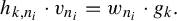 $$ \begin{align*} h_{k,n_i}\cdot v_{n_i}=w_{n_i}\cdot g_k. \end{align*} $$
Let $\tilde {g}_k$
be the lift of
$\tilde {g}_k$
be the lift of $g_k$
through
$g_k$
through $f^{n_i}$
starting from the terminal point of
$f^{n_i}$
starting from the terminal point of $w_{n_i}$
. Let
$w_{n_i}$
. Let $\tilde {\delta }_e$
and
$\tilde {\delta }_e$
and $\tilde {\delta }_{e'}$
be the parts of
$\tilde {\delta }_{e'}$
be the parts of $\tilde {g}_k$
where
$\tilde {g}_k$
where $\delta _e$
and
$\delta _e$
and $\delta _{e'}$
are lifted. We specify
$\delta _{e'}$
are lifted. We specify $w_{n_i}$
as an element of
$w_{n_i}$
as an element of $X^{\otimes n_i}$
satisfying the following: the curve
$X^{\otimes n_i}$
satisfying the following: the curve $g_k$
with
$g_k$
with $\delta _e$
and
$\delta _e$
and $\delta _{e'}$
being truncated is
$\delta _{e'}$
being truncated is $S_{\mathcal {R}}$
-combinatorially equivalent to
$S_{\mathcal {R}}$
-combinatorially equivalent to $\tilde {g}_k$
with
$\tilde {g}_k$
with $\tilde {\delta }_e$
and
$\tilde {\delta }_e$
and $\tilde {\delta }_{e'}$
being truncated. See Figure 6.
$\tilde {\delta }_{e'}$
being truncated. See Figure 6.
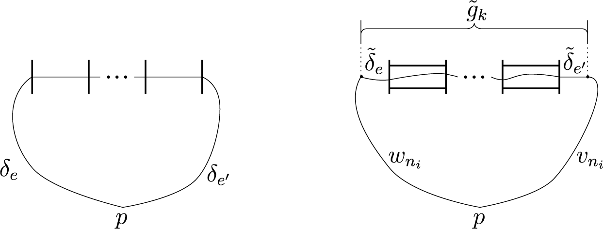
Figure 6 The left figure is $g_k$
drawn in
$g_k$
drawn in $S_{\mathcal {R}}$
, and the right figure is
$S_{\mathcal {R}}$
, and the right figure is $h_{k,n_i}$
drawn in
$h_{k,n_i}$
drawn in $\mathcal {R}^{n_i}(S_{\mathcal {R}})$
. The bold line segments are portions of
$\mathcal {R}^{n_i}(S_{\mathcal {R}})$
. The bold line segments are portions of $1$
-skeletons of
$1$
-skeletons of $S_{\mathcal {R}}$
and
$S_{\mathcal {R}}$
and $\mathcal {R}^{n_i}(S_{\mathcal {R}})$
.
$\mathcal {R}^{n_i}(S_{\mathcal {R}})$
.
Then $h_{k,n_i}$
and
$h_{k,n_i}$
and $g_k$
differ by the pre- and post-composition with loops
$g_k$
differ by the pre- and post-composition with loops $w_{n_i}\cdot \tilde {\delta }_e \cdot \overline {\delta }_e$
and
$w_{n_i}\cdot \tilde {\delta }_e \cdot \overline {\delta }_e$
and $\overline {\delta }_{e'} \cdot \delta _{e'} \cdot \overline {v}_{n_i}$
. We have: (1) a uniform upper bound on the homotopic length of
$\overline {\delta }_{e'} \cdot \delta _{e'} \cdot \overline {v}_{n_i}$
. We have: (1) a uniform upper bound on the homotopic length of $v_{n_i}$
and
$v_{n_i}$
and $w_{n_i}$
(in the projection to the Böttcher expanding map) by Lemma 5.11; (2) a uniform upper bound on the intersection between
$w_{n_i}$
(in the projection to the Böttcher expanding map) by Lemma 5.11; (2) a uniform upper bound on the intersection between $\delta _e$
and
$\delta _e$
and $S_{\mathcal {R}}^{(1)}$
; and (3) the upper bound in item (2) is also an upper bound of the intersection between any level-n lift
$S_{\mathcal {R}}^{(1)}$
; and (3) the upper bound in item (2) is also an upper bound of the intersection between any level-n lift $\tilde {\delta }_e$
and
$\tilde {\delta }_e$
and $\mathcal {R}^n(S_{\mathcal {R}})^{(1)}$
. Therefore, we have
$\mathcal {R}^n(S_{\mathcal {R}})^{(1)}$
. Therefore, we have $\|w_{n_i}\cdot \tilde {\delta }_e \cdot \overline {\delta }_e\|, \|\overline {\delta }_{e'} \cdot \delta _{e'} \cdot \overline {v}_{n_i}\|< C/2$
for some C so that
$\|w_{n_i}\cdot \tilde {\delta }_e \cdot \overline {\delta }_e\|, \|\overline {\delta }_{e'} \cdot \delta _{e'} \cdot \overline {v}_{n_i}\|< C/2$
for some C so that $d(g_k,h_{k,n_i})<C$
. Since there are only finitely many elements of
$d(g_k,h_{k,n_i})<C$
. Since there are only finitely many elements of $\pi _1(S^2,A,\textrm {ord})$
within the distance C from
$\pi _1(S^2,A,\textrm {ord})$
within the distance C from $g_k$
, there exists
$g_k$
, there exists $h_k$
such that
$h_k$
such that $h_k=h_{k,n_i}$
for infinitely many i terms.
$h_k=h_{k,n_i}$
for infinitely many i terms.
Step 2: Proof of $\|h_k\|\to \infty $
. Let
$\|h_k\|\to \infty $
. Let $g_k$
and
$g_k$
and $h_k$
be as defined in Step 1. Since
$h_k$
be as defined in Step 1. Since $d(h_k,g_k)<C$
, it suffices to show
$d(h_k,g_k)<C$
, it suffices to show $\|g_k\|\to \infty $
as k tends to
$\|g_k\|\to \infty $
as k tends to $\infty $
.
$\infty $
.
Let $e_0$
and
$e_0$
and $e_k$
be the level-
$e_k$
be the level- $0$
edges whose midpoints are the endpoints of
$0$
edges whose midpoints are the endpoints of $\gamma ^0([0,k])$
so that
$\gamma ^0([0,k])$
so that $g_k=\delta _{e_0} \cdot \gamma ^0([0,k]) \cdot \overline {\delta }_{e_k}$
. Then
$g_k=\delta _{e_0} \cdot \gamma ^0([0,k]) \cdot \overline {\delta }_{e_k}$
. Then $\|g_k\|\to \infty $
follows from the condition that
$\|g_k\|\to \infty $
follows from the condition that $\gamma ^0$
is homotopically infinite.
$\gamma ^0$
is homotopically infinite.
6 Non-expanding spines
From Theorem 5.1, we know that the existence of a Levy cycle is equivalent to the existence of a genealogical sequence of homotopically infinite recurrent non-expanded curves. Then, how can we detect the existence of such a sequence? The direct search for the genealogical sequence could be more complicated than the search for the Levy cycle. One motivation for non-expanding spines is to have a simpler object with which we can efficiently detect the genealogical sequence.
Since recurrent non-expanded level-n curves are concatenations of level-n recurrent bones, that is, the bones of level-n recurrent bands, it is natural to consider the union of level-n recurrent bones. The level-n non-expanding spine $N^n$
is, roughly speaking, the union of level-n recurrent bones equipped with a natural train-track structure.
$N^n$
is, roughly speaking, the union of level-n recurrent bones equipped with a natural train-track structure.
6.0.1 Motivation for the use of train-tracks
Let us see Figure 7. Let t denote the hexagonal tile and $e_1,e_2,e_3$
denote three of its boundary edges. Suppose that
$e_1,e_2,e_3$
denote three of its boundary edges. Suppose that $b_1=(t;e_1,e_2)$
and
$b_1=(t;e_1,e_2)$
and $b_2=(t;e_1,e_3)$
are level-0 recurrent bands so that each has two level-1 recurrent subbands of type
$b_2=(t;e_1,e_3)$
are level-0 recurrent bands so that each has two level-1 recurrent subbands of type $b_1$
and
$b_1$
and $b_2$
. Then each level-1 recurrent subband of type
$b_2$
. Then each level-1 recurrent subband of type $b_1$
or
$b_1$
or $b_2$
has two level-
$b_2$
has two level- $2$
recurrent subbands of type
$2$
recurrent subbands of type $b_1$
and
$b_1$
and $b_2$
. Assume that we draw the bones of these bands. At level-0, we have two curves each of which joins
$b_2$
. Assume that we draw the bones of these bands. At level-0, we have two curves each of which joins $e_1$
to
$e_1$
to $e_2$
or
$e_2$
or $e_3$
. As a ‘collection’ of these two curves, we might consider a tripod whose leaves are on
$e_3$
. As a ‘collection’ of these two curves, we might consider a tripod whose leaves are on $e_1,e_2,$
and
$e_1,e_2,$
and $e_3$
. However, the tripod contains an unintended curve which joins
$e_3$
. However, the tripod contains an unintended curve which joins $e_2$
to
$e_2$
to $e_3$
. To exclude such a curve, we use the idea of train-tracks, which makes the curve joining
$e_3$
. To exclude such a curve, we use the idea of train-tracks, which makes the curve joining $e_2$
and
$e_2$
and $e_3$
illegal.
$e_3$
illegal.
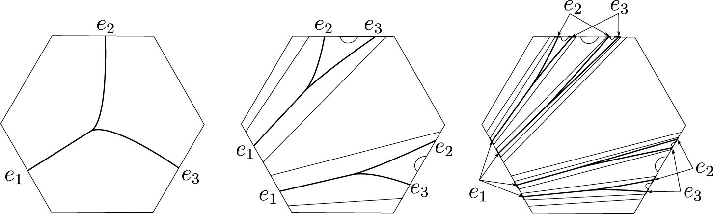
Figure 7 Train-track structures on non-expanding spines.
6.1 Train-track
Let G be a graph and $v\in G$
be a point, which could be a vertex or a point in the interior of an edge. A direction at v is a germ of continuous curves starting from v. The number of directions at v is equal to the number of connected components of
$v\in G$
be a point, which could be a vertex or a point in the interior of an edge. A direction at v is a germ of continuous curves starting from v. The number of directions at v is equal to the number of connected components of $U\setminus \{v\}$
, where U is a sufficiently small neighborhood of v. Denote the set of directions at v by
$U\setminus \{v\}$
, where U is a sufficiently small neighborhood of v. Denote the set of directions at v by $D_v$
.
$D_v$
.
Definition 6.1. (Train-tracks and gates)
Let G be a finite graph. For any vertex v of G, a train-track structure $\tau $
on G is an assignment of an equivalence relation on
$\tau $
on G is an assignment of an equivalence relation on $D_v$
for each
$D_v$
for each $v\in \operatorname{Vert}(G)$
. A train-track is a finite graph G equipped with a train-track structure
$v\in \operatorname{Vert}(G)$
. A train-track is a finite graph G equipped with a train-track structure $\tau $
and denoted by
$\tau $
and denoted by $(G,\tau )$
. For any
$(G,\tau )$
. For any $v\in G\setminus \operatorname{Vert}(G)$
,
$v\in G\setminus \operatorname{Vert}(G)$
, $D_v$
has two directions and we define each equivalence class of
$D_v$
has two directions and we define each equivalence class of $D_v$
to have each direction. Below is a list of definitions regarding train-tracks.
$D_v$
to have each direction. Below is a list of definitions regarding train-tracks.
-
• Each equivalence class of
$D_v$
is called a gate at v. -
• A train path is an oriented curve
$\gamma $
in G such that at every vertex v, the gate through which
$\gamma $
comes to v is different from the gate through which
$\gamma $
goes out.


Definition 6.2. (Train-track map)
Let $T_1=(G_1,\tau _1)$
and
$T_1=(G_1,\tau _1)$
and $T_2=(G_2,\tau _2)$
be train-tracks. A train-track map
$T_2=(G_2,\tau _2)$
be train-tracks. A train-track map $\phi :T_1\to T_2$
is a continuous map
$\phi :T_1\to T_2$
is a continuous map $\phi :G_1\to G_2$
that is locally injective on each edge such that for every
$\phi :G_1\to G_2$
that is locally injective on each edge such that for every $v \in G_1$
and
$v \in G_1$
and $d_1,d_2\in D_v$
,
$d_1,d_2\in D_v$
, $\phi (d_1)$
and
$\phi (d_1)$
and $\phi (d_2)$
are in the same gate at
$\phi (d_2)$
are in the same gate at $\phi (v)$
if
$\phi (v)$
if $d_1$
and
$d_1$
and $d_2$
are in the same gate.
$d_2$
are in the same gate.
Definition 6.3. (Homotopy relative to
$(\partial S,X)$
)

Let $f,g:(S,\partial S, X) \to (S,\partial S, X)$
be two continuous maps. We say that f and g are homotopic (respectively isotopic) relative to
$f,g:(S,\partial S, X) \to (S,\partial S, X)$
be two continuous maps. We say that f and g are homotopic (respectively isotopic) relative to $(\partial S,X)$
if there is a homotopy (respectively isotopy)
$(\partial S,X)$
if there is a homotopy (respectively isotopy) $\{H_t:S\to S\}_{t\in [0,1]}$
such that:
$\{H_t:S\to S\}_{t\in [0,1]}$
such that:
-
•
$H_0=f$
and
$H_1=g$
; -
•
$H_t|_X:X\to X=\mathrm{id}_X:X\to X$
; and -
• for every
$t\in [0,1]$
,
$H_t$
sends every connected component of
$\partial S \setminus X$
to itself.


Definition 6.4. (Graphs properly embedded in
$(S,\partial S,X)$
)

Let S be a compact surface with a finite set of marked points X. Some marked points may be on the boundary $\partial S$
. A graph
$\partial S$
. A graph $G\subset S$
is properly embedded in
$G\subset S$
is properly embedded in $(S,\partial S, X)$
if
$(S,\partial S, X)$
if $(G,\partial G)$
is properly embedded in
$(G,\partial G)$
is properly embedded in $(S,\partial S)$
and
$(S,\partial S)$
and $G \subset S\setminus X$
, where
$G \subset S\setminus X$
, where $\partial G$
is the set of leaves of G. We say that two graphs G and H properly embedded in
$\partial G$
is the set of leaves of G. We say that two graphs G and H properly embedded in $(S, \partial S, X)$
are homotopic (respectively isotopic) if there is an ambient homotopy
$(S, \partial S, X)$
are homotopic (respectively isotopic) if there is an ambient homotopy $\{H_t:S\to S\}_{t\in [0,1]}$
(respectively isotopy) relative to
$\{H_t:S\to S\}_{t\in [0,1]}$
(respectively isotopy) relative to $(\partial S,X)$
such that
$(\partial S,X)$
such that $H_0=id_S:S\to S$
and
$H_0=id_S:S\to S$
and $H_1(G)=H$
.
$H_1(G)=H$
.
Definition 6.5. (Train-tracks in surfaces)
Let S be a compact surface possibly with boundary $\partial S$
and a finite set of marked points
$\partial S$
and a finite set of marked points $X\subset S$
. By a train-track in
$X\subset S$
. By a train-track in $(S,\partial S, X)$
, we mean a train-track
$(S,\partial S, X)$
, we mean a train-track $(G,\tau )$
of a graph G satisfying (1) G is properly embedded in
$(G,\tau )$
of a graph G satisfying (1) G is properly embedded in $(S,\partial S,X)$
and (2) the train-track structure
$(S,\partial S,X)$
and (2) the train-track structure $\tau $
is compatible with the planar structure in the following sense: for every
$\tau $
is compatible with the planar structure in the following sense: for every $v\in \operatorname{Vert}(G)$
,
$v\in \operatorname{Vert}(G)$
, $D_v$
has a cyclic order defined by a local orientation of S near v. Then every gate at v consists of edges that are consecutive with respect to the cycle order. We note that the consecutiveness is independent of the choice of local orientations, and thus the definition also works for non-orientable surface S.
$D_v$
has a cyclic order defined by a local orientation of S near v. Then every gate at v consists of edges that are consecutive with respect to the cycle order. We note that the consecutiveness is independent of the choice of local orientations, and thus the definition also works for non-orientable surface S.
Remark 6.6. Train-tracks are commonly used to describe complicated curves or foliations. For these purposes, train-tracks are often assumed to have additional properties, such as that every vertex v has degree $3$
, the number of gates at each vertex is always two, and the complement of a train-track is hyperbolic, all of which are not assumed in this article. See [Reference Penner and HarerPH92].
$3$
, the number of gates at each vertex is always two, and the complement of a train-track is hyperbolic, all of which are not assumed in this article. See [Reference Penner and HarerPH92].
Definition 6.7. (Carrying between train-tracks)
Let S be a compact surface with a finite set of marked points $X \subset S$
. Let
$X \subset S$
. Let $T_1$
and
$T_1$
and $T_2$
be train-tracks in
$T_2$
be train-tracks in $(S,\partial S, X)$
. We say that
$(S,\partial S, X)$
. We say that $T_2$
carries
$T_2$
carries $T_1$
if there is a train-track map
$T_1$
if there is a train-track map $\phi :T_1 \to T_2$
such that
$\phi :T_1 \to T_2$
such that $\phi $
can be extended to a map
$\phi $
can be extended to a map $\phi :S\to S$
that is ambient homotopic relative to
$\phi :S\to S$
that is ambient homotopic relative to $(\partial S,X)$
to the identity map. In particular, considering a possibly non-closed curve
$(\partial S,X)$
to the identity map. In particular, considering a possibly non-closed curve $\gamma :I\to S$
properly embedded in
$\gamma :I\to S$
properly embedded in $(S,\partial S,X)$
as a train-track with no vertex, we can say that a train-track T carries
$(S,\partial S,X)$
as a train-track with no vertex, we can say that a train-track T carries $\gamma $
if
$\gamma $
if $\gamma $
is contained in S up to homotopy in
$\gamma $
is contained in S up to homotopy in $(S,\partial S, X)$
.
$(S,\partial S, X)$
.
Definition 6.8. (Homotopically infinite train-tracks)
Let $(S^2,A,\textrm {ord})$
be a hyperbolic orbisphere. A train-track T in
$(S^2,A,\textrm {ord})$
be a hyperbolic orbisphere. A train-track T in $(S^2,A)$
is homotopically infinite if T carries a homotopically infinite closed curve with respect to the orbisphere structure
$(S^2,A)$
is homotopically infinite if T carries a homotopically infinite closed curve with respect to the orbisphere structure $\textrm {ord}$
.
$\textrm {ord}$
.
6.2 Decomposition of graph with crossing condition on the unit disk
In this subsection, we investigate a graph theoretic property which will be used to define non-expanding spines.
Let us consider a unit disk in the Euclidean plane and its boundary circle. A chord is an Euclidean line segment joining to a point on the circle. We say that two chords intersect if they intersect in the interior of the disk. Similarly, for two sets of chords $S_1$
and
$S_1$
and $S_2$
, we say that
$S_2$
, we say that $S_1$
and
$S_1$
and $S_2$
intersect if there exist chords
$S_2$
intersect if there exist chords $s_1\in S_1$
and
$s_1\in S_1$
and $s_2 \in S_2$
so that
$s_2 \in S_2$
so that $s_1$
and
$s_1$
and $s_2$
intersect.
$s_2$
intersect.
Fix $n\ge 2$
points on the boundary circle C of a unit disk. There are
$n\ge 2$
points on the boundary circle C of a unit disk. There are $n(n-1)/2$
different chords joining the n points. Let S be a collection of these chords. The collection S can also be considered as a graph. We abuse notation and use S to indicate the graph also. A decomposition of a graph G is a collection of subgraphs
$n(n-1)/2$
different chords joining the n points. Let S be a collection of these chords. The collection S can also be considered as a graph. We abuse notation and use S to indicate the graph also. A decomposition of a graph G is a collection of subgraphs $G_1,G_2,\ldots , G_k$
which gives a partition on the set of edges.
$G_1,G_2,\ldots , G_k$
which gives a partition on the set of edges.
Lemma 6.9. Let $v_1,v_2,\ldots ,v_n$
be
$v_1,v_2,\ldots ,v_n$
be $n\ge 2$
points on a circle. Let S be a collection of chords joining pairs of
$n\ge 2$
points on a circle. Let S be a collection of chords joining pairs of $v_i$
terms. Suppose S satisfies the following crossing condition.
$v_i$
terms. Suppose S satisfies the following crossing condition.
-
(Crossing condition) If two chords
$s,s'\in S$
are intersecting, then all the six chords joining any pairs of four endpoints of
$s,s'$
are also contained in S.


Then, as a graph, S is decomposed into mutually non-intersecting (1) complete graphs with at least four vertices and (2) chords, which can also be considered as complete graphs with two vertices.
Proof. The condition implies that if S contains two intersecting chords, then it contains the complete graph of the four vertices. Suppose that a subset $S'$
of S forms a complete graph. We first show that if there is a chord s in
$S'$
of S forms a complete graph. We first show that if there is a chord s in $S \setminus S'$
that intersects
$S \setminus S'$
that intersects $S'$
, then S also contains the complete graph generated by
$S'$
, then S also contains the complete graph generated by $S' \cup \{s\}$
. Denote by v and w the endpoints of s. Since s intersects
$S' \cup \{s\}$
. Denote by v and w the endpoints of s. Since s intersects $S'$
, there exists
$S'$
, there exists $s'$
that intersects s. Let
$s'$
that intersects s. Let $v'$
and
$v'$
and $w'$
denote the endpoints of
$w'$
denote the endpoints of $s'$
. For any vertex
$s'$
. For any vertex $u'$
of
$u'$
of $S'$
, as a graph, which is not v or w, either
$S'$
, as a graph, which is not v or w, either $\overline {u'v'}$
or
$\overline {u'v'}$
or $\overline {u'w'}$
intersects s. In particular, by the crossing condition, the chords
$\overline {u'w'}$
intersects s. In particular, by the crossing condition, the chords $\overline {u'v}$
and
$\overline {u'v}$
and $\overline {u'w}$
are contained in S. Since
$\overline {u'w}$
are contained in S. Since $u'$
was taken arbitrarily, the complete graph with vertex set
$u'$
was taken arbitrarily, the complete graph with vertex set $\operatorname{Vert}(S')\cup \{v,w\}$
is also contained in S.
$\operatorname{Vert}(S')\cup \{v,w\}$
is also contained in S.
Then every complete graph in S can be extended until when it does not intersect other chords in S, which proves the conclusion.
Proposition 6.10. Let t be an n-gon for $n\ge 2$
. For a curve
$n\ge 2$
. For a curve $\gamma $
properly embedded in
$\gamma $
properly embedded in $(t,\partial t, \operatorname{Vert}(t))$
, we call the boundary edges of t that contain the endpoints of
$(t,\partial t, \operatorname{Vert}(t))$
, we call the boundary edges of t that contain the endpoints of $\gamma $
the side edges of
$\gamma $
the side edges of $\gamma $
. Let S be a collection of homotopy classes of properly embedded curves joining different boundary edges. Suppose that S satisfies the following crossing condition.
$\gamma $
. Let S be a collection of homotopy classes of properly embedded curves joining different boundary edges. Suppose that S satisfies the following crossing condition.
-
(Crossing condition) If
$\langle [\alpha ], [\beta ]\rangle=1$
, then S contains the six homotopy classes of curves connecting any pairs of the four side edges of
$\alpha $
and
$\beta $
.


Then there is a train-track T properly embedded in $(t,\partial t, \operatorname{Vert}(t))$
such that for any curve
$(t,\partial t, \operatorname{Vert}(t))$
such that for any curve $\gamma $
properly embedded in
$\gamma $
properly embedded in $(t,\partial t, \operatorname{Vert}(t))$
,
$(t,\partial t, \operatorname{Vert}(t))$
, $\gamma $
is carried by T if and only if
$\gamma $
is carried by T if and only if $[\gamma ]\in S$
.
$[\gamma ]\in S$
.
Proof. We may consider t as a closed disk. We also choose a point on each boundary edge and take a representative of a homotopy class of curves properly embedded in t as a chord joining the chosen points on the edges. Then S can be considered as a graph, see Figure 8. By Lemma 6.9, S is decomposed into complete graphs (with at least four vertices) and curves that are mutually non-intersecting.
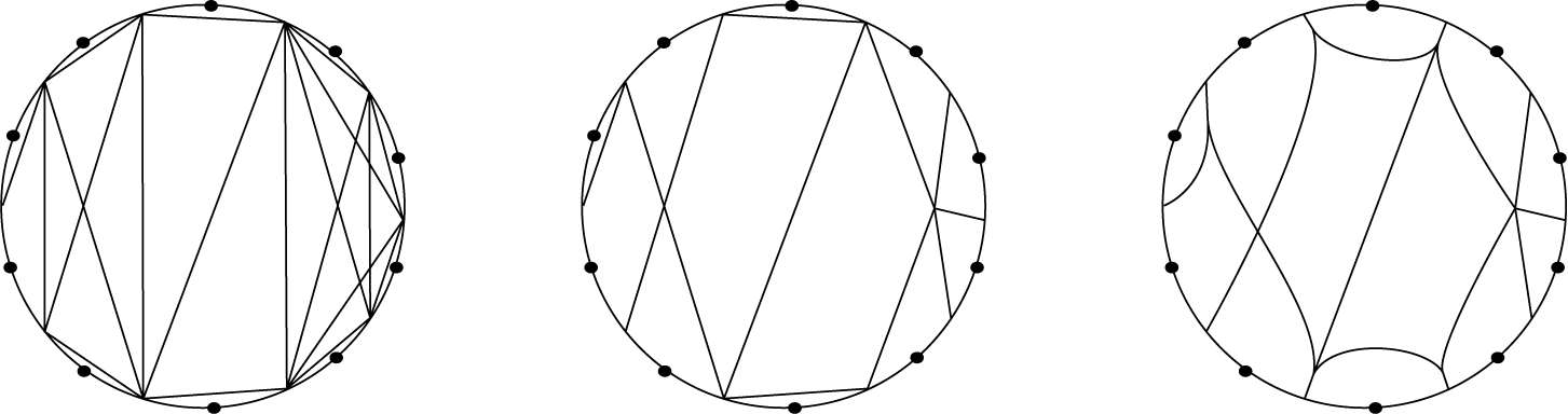
Figure 8 Transformation from a graph to a train-track. The dots on the boundary are vertices of a polygon. The graph contains two complete graphs with more than three vertices. These graphs are transformed into star-like trees of degree $4$
and
$4$
and $5$
, respectively. We ‘zip-up’ at boundary points to define a train-track structure.
$5$
, respectively. We ‘zip-up’ at boundary points to define a train-track structure.
Suppose that $S'\subset S$
forms a complete graph with
$S'\subset S$
forms a complete graph with $k\ge 4$
vertices in the decomposition. Then we transform
$k\ge 4$
vertices in the decomposition. Then we transform $S'$
into a star-like tree
$S'$
into a star-like tree $T'$
whose leaves are the k vertices of
$T'$
whose leaves are the k vertices of $S'$
. We transform all the complete graphs in the decomposition of S to star-like trees as above, see the middle figure in Figure 8. Then we have a graph that is the union of some star-like trees and curves which can intersect only in the boundary of t.
$S'$
. We transform all the complete graphs in the decomposition of S to star-like trees as above, see the middle figure in Figure 8. Then we have a graph that is the union of some star-like trees and curves which can intersect only in the boundary of t.
We define a train-track as follows.
-
(1) Let v be the center of a star-like tree. We define gates at v in such a way that each gate has only one edge.
-
(2) At each intersection in
$\partial t$
, we zip the intersecting curves up a little bit as in the right figure in Figure 8. More precisely, assume that k edges, say
$e_1,e_2,\ldots e_k$
intersect at a boundary point p. The transformation generates one vertex v of degree
$d+1$
; the vertex v is incident to the (deformed) k edges
$e_1,e_2,\ldots ,e_k$
, and to one new edge, say e, which joins p to v. There are two gates at v:
$\{\textrm {the direction along}~e_i~|~i\in [1,k]_{\mathbb {Z}}\}$
and
$\{\textrm {the direction along}~e\}$
.


It is immediate from the construction that the train-track satisfies the desired property.
6.3 Non-expanding spines of tiles
Let t be a level- $0$
tile of a finite subdivision rule
$0$
tile of a finite subdivision rule $\mathcal {R}$
and
$\mathcal {R}$
and $n\ge 0$
. For simplicity, we assume that t is homeomorphic to a closed 2-disc, that is, boundary edges are not identified. We will define the level-n non-expanding spine of t as a train-track properly embedded in t which is roughly speaking the union of level-n recurrent bones in t. If boundary edges are identified, we first define a train-track in the closed 2-disc
$n\ge 0$
. For simplicity, we assume that t is homeomorphic to a closed 2-disc, that is, boundary edges are not identified. We will define the level-n non-expanding spine of t as a train-track properly embedded in t which is roughly speaking the union of level-n recurrent bones in t. If boundary edges are identified, we first define a train-track in the closed 2-disc $\textbf {t}$
, which is the domain of the characteristic map
$\textbf {t}$
, which is the domain of the characteristic map $\phi _t:\textbf {t}\to t$
, and then define the non-expanding spine as the image of the train-track by
$\phi _t:\textbf {t}\to t$
, and then define the non-expanding spine as the image of the train-track by $\phi _t$
.
$\phi _t$
.
For a level- $0$
tile t and a level-n band
$0$
tile t and a level-n band $b^n=(t^n;e_1^n,e_2^n)$
, we say that
$b^n=(t^n;e_1^n,e_2^n)$
, we say that $b^n$
is a subband of t if
$b^n$
is a subband of t if $t^n\subset t$
and
$t^n\subset t$
and $e^n_1,e^n_2\subset \partial t$
. We say that two level-n subbands
$e^n_1,e^n_2\subset \partial t$
. We say that two level-n subbands $b^n_0$
and
$b^n_0$
and $b^n_1$
of a level-
$b^n_1$
of a level- $0$
tile t intersect if their bones have non-zero intersection number, which must be one, of the homotopy classes of curves properly embedded in
$0$
tile t intersect if their bones have non-zero intersection number, which must be one, of the homotopy classes of curves properly embedded in $(t, \mathcal {R}^n(\partial t), \operatorname{Vert}(\mathcal {R}^n(\partial t)))$
. It is immediate that if two level-n subbands
$(t, \mathcal {R}^n(\partial t), \operatorname{Vert}(\mathcal {R}^n(\partial t)))$
. It is immediate that if two level-n subbands $b^n_0$
and
$b^n_0$
and $b^n_1$
intersect, then they are bands of the same level-n subtile of t.
$b^n_1$
intersect, then they are bands of the same level-n subtile of t.
The next lemma, in particular the property (3), implies that the set of level-n recurrent bones of t satisfies the crossing condition in the statement of Lemma 6.9 or Proposition 6.10.
Lemma 6.11. Let t be a level-0 tile of a finite subdivision rule. For a level- $0$
recurrent band
$0$
recurrent band $b_0=(t;e_{0,1},e_{0,2})$
, let
$b_0=(t;e_{0,1},e_{0,2})$
, let $A^0:=\{b_i=(t;e_{i,1},e_{i,2})~|~i=1,\ldots , k\}$
be the collection of level-
$A^0:=\{b_i=(t;e_{i,1},e_{i,2})~|~i=1,\ldots , k\}$
be the collection of level- $0$
recurrent bands that intersect
$0$
recurrent bands that intersect $b_0$
. Suppose that
$b_0$
. Suppose that $A^0$
is non-empty. Then we have the following properties.
$A^0$
is non-empty. Then we have the following properties.
-
(1) For any
$n \ge 0$
and
$i\in [0,k]_{\mathbb {Z}}$
, there is a level-n subtile
$t^n$
of t such that each
$b_i$
has a unique level-n subband
$b^n_i=(t^n;e^n_{i,1},e^n_{i,2})$
, which is also recurrent. That is, in the directed graph
$\mathcal {B}$
of bands,
$[b_i]$
belongs to only one cycle, say C, and there is no directed path from C to another cycle. -
(2) There exists
$p>0$
such that
$b^{np}_i$
is of type
$b_i$
for every
$i\in [0,k]_{\mathbb {Z}}$
and any
$n>0$
. Moreover, p can be chosen as the common period of the cycles in
$\mathcal {B}$
containing
$[b_i]$
terms. -
(3) For every pair
$(i,j), (i',j') \in [0,k]_{\mathbb {Z}} \times \{1,2\}$
with
$e_{i,j}\neq e_{i',j'}$
, the band
$(t^n;e^n_{i,j},e^n_{i',j'})$
is a level-n recurrent subband of t for every
$n\ge 0$
.


Proof. For any $n>0$
, every level-n child of
$n>0$
, every level-n child of $b_0$
intersects any level-n child of any
$b_0$
intersects any level-n child of any $b_i$
. Hence, all the level-n children of
$b_i$
. Hence, all the level-n children of $b_0,b_1,\ldots ,b_k$
are bands of the same level-n subtile, say
$b_0,b_1,\ldots ,b_k$
are bands of the same level-n subtile, say $t^n$
, of t.
$t^n$
, of t.
For $n>0$
, we define a set
$n>0$
, we define a set $A^n$
as the collection of level-n recurrent subbands of the level-
$A^n$
as the collection of level-n recurrent subbands of the level- $0$
bands in
$0$
bands in $A^0$
. Since every recurrent level-n band has at least one recurrent child at each higher level, we have a sequence of surjections
$A^0$
. Since every recurrent level-n band has at least one recurrent child at each higher level, we have a sequence of surjections $A^0\leftarrow A^1\leftarrow \cdots $
which map recurrent subbands to their parents.
$A^0\leftarrow A^1\leftarrow \cdots $
which map recurrent subbands to their parents.
To show the uniqueness in property (1), it suffices to show that the surjections ( $A^{n+1}\to A^n$
) are actually bijections. Since
$A^{n+1}\to A^n$
) are actually bijections. Since $b_0$
is recurrent, for infinitely many
$b_0$
is recurrent, for infinitely many $n_0>0$
, the level-
$n_0>0$
, the level- $0$
band
$0$
band $b_0$
has a level-
$b_0$
has a level- $n_0$
recurrent subband
$n_0$
recurrent subband $b^{n_0}_0$
of type
$b^{n_0}_0$
of type $b_0$
. In particular,
$b_0$
. In particular, $t^{n_0}$
is of type
$t^{n_0}$
is of type $\textbf {t}$
. Then the types of level-
$\textbf {t}$
. Then the types of level- $n_0$
subbands of
$n_0$
subbands of $b_i$
for
$b_i$
for $i\in [1,k]_{\mathbb {Z}}$
injectively correspond to
$i\in [1,k]_{\mathbb {Z}}$
injectively correspond to $b_j$
for
$b_j$
for $j\in [1,k]_{\mathbb {Z}}$
. This implies that
$j\in [1,k]_{\mathbb {Z}}$
. This implies that $A^0\leftarrow \cdots \leftarrow A^{n_0}$
is a sequence of bijections. Since there are infinitely many such
$A^0\leftarrow \cdots \leftarrow A^{n_0}$
is a sequence of bijections. Since there are infinitely many such $n_0$
terms,
$n_0$
terms, $A^0\leftarrow A^1 \leftarrow \cdots $
is a sequence of bijections also.
$A^0\leftarrow A^1 \leftarrow \cdots $
is a sequence of bijections also.
(2) Let p be the least positive integer satisfying that $b^p_0=(t^p;e^p_{0,1},e^p_{0,2})$
is of type
$b^p_0=(t^p;e^p_{0,1},e^p_{0,2})$
is of type $b_0=(t;e_{0,1},e_{0,2})$
. Such a p exists because
$b_0=(t;e_{0,1},e_{0,2})$
. Such a p exists because $b_0$
is recurrent. We claim that
$b_0$
is recurrent. We claim that $b^{np}_i$
is of type
$b^{np}_i$
is of type $b_i$
for every
$b_i$
for every $n \ge 1$
. Here is a sketch of the proof and we leave the details to the reader. Since tiles and bands are objects embedded in the sphere, we can define an order on
$n \ge 1$
. Here is a sketch of the proof and we leave the details to the reader. Since tiles and bands are objects embedded in the sphere, we can define an order on $A^n$
according to how close
$A^n$
according to how close $b^n_i$
is to
$b^n_i$
is to $b^n_0$
. The order is preserved by the bijections
$b^n_0$
. The order is preserved by the bijections $A^{m+1}\to A^m$
we discussed in property (1), which implies
$A^{m+1}\to A^m$
we discussed in property (1), which implies $b^{np}_i$
is of type
$b^{np}_i$
is of type $b_i$
for every
$b_i$
for every $n>0$
and
$n>0$
and $i\in [1,k]_{\mathbb {Z}}$
. By exchanging the roles of
$i\in [1,k]_{\mathbb {Z}}$
. By exchanging the roles of $b_0$
with
$b_0$
with $b_i$
for any
$b_i$
for any $i\in [1,k]_{\mathbb {Z}}$
, we obtain that p is the common period of the cycles in
$i\in [1,k]_{\mathbb {Z}}$
, we obtain that p is the common period of the cycles in $\mathcal {B}$
containing
$\mathcal {B}$
containing $[b_i]$
terms.
$[b_i]$
terms.
(3) Let $p>0$
be the number determined in property (2). It follows from property (2) that for every
$p>0$
be the number determined in property (2). It follows from property (2) that for every $n>0$
and
$n>0$
and $(i,j)\in [0,k]_{\mathbb {Z}} \times \{1,2\}$
, the level-
$(i,j)\in [0,k]_{\mathbb {Z}} \times \{1,2\}$
, the level- $np$
subtile
$np$
subtile $t^{np}$
is of type
$t^{np}$
is of type $\textbf {t}$
and its boundary edge
$\textbf {t}$
and its boundary edge $e^{np}_{i,j}$
is a subedge of
$e^{np}_{i,j}$
is a subedge of $e_{i,j}$
and of type
$e_{i,j}$
and of type $\textbf {e}_{i,j}$
. Hence, for every pair
$\textbf {e}_{i,j}$
. Hence, for every pair $(i,j), (i',j') \in [0,k] \times \{1,2\}$
with
$(i,j), (i',j') \in [0,k] \times \{1,2\}$
with $e_{i,j}\neq e_{i',j'}$
, the level-
$e_{i,j}\neq e_{i',j'}$
, the level- $0$
band
$0$
band $(t;e_{i,j},e_{i',j'})$
has a level-
$(t;e_{i,j},e_{i',j'})$
has a level- $np$
subband
$np$
subband $(t^{np},e^{np}_{i,j},e^{np}_{i',j'})$
which is of type
$(t^{np},e^{np}_{i,j},e^{np}_{i',j'})$
which is of type $(t;e_{i,j},e_{i',j'})$
. Then
$(t;e_{i,j},e_{i',j'})$
. Then $(t^n,e^n_{i,j},e^n_{i',j'})$
is recurrent for every
$(t^n,e^n_{i,j},e^n_{i',j'})$
is recurrent for every $n\ge 1$
.
$n\ge 1$
.
Proposition 6.12. Let t be a level-0 tile of a finite subdivision rule $\mathcal {R}$
. Then there is a train-track
$\mathcal {R}$
. Then there is a train-track $T^n(t)$
whose underlying graph is properly embedded in
$T^n(t)$
whose underlying graph is properly embedded in $(t,\mathcal {R}^n(\partial t),\operatorname{Vert}(\mathcal {R}^n(\partial t)))$
such that any curve
$(t,\mathcal {R}^n(\partial t),\operatorname{Vert}(\mathcal {R}^n(\partial t)))$
such that any curve $\gamma $
properly embedded in
$\gamma $
properly embedded in $(t,\mathcal {R}^n(\partial t), \operatorname{Vert}(\mathcal {R}^n(\partial t)))$
is carried by
$(t,\mathcal {R}^n(\partial t), \operatorname{Vert}(\mathcal {R}^n(\partial t)))$
is carried by $T^n(t)$
if and only if
$T^n(t)$
if and only if $\gamma $
is the bone of a level-n recurrent subband of t.
$\gamma $
is the bone of a level-n recurrent subband of t.
Proof. We first assume that the tile t is a closed disk, that is, its boundary edges are not identified. It follows from Lemma 6.11(3) that the collection of spines $B^n(t)$
satisfies the crossing condition in Proposition 6.10. Hence, we have the desired train-tack by Proposition 6.10.
$B^n(t)$
satisfies the crossing condition in Proposition 6.10. Hence, we have the desired train-tack by Proposition 6.10.
If t is not a closed disk, we can use Proposition 6.10 for its domain $\textbf {t}$
, which is a closed disk, of the characteristic map
$\textbf {t}$
, which is a closed disk, of the characteristic map $\phi _t:\textbf {t}\to t$
to obtain a train-track
$\phi _t:\textbf {t}\to t$
to obtain a train-track $T^n(\textbf {t})$
in
$T^n(\textbf {t})$
in $\textbf {t}$
. Then we define
$\textbf {t}$
. Then we define $T^n(t)$
as the
$T^n(t)$
as the $\phi _t$
-image of
$\phi _t$
-image of $T^n(\textbf {t})$
. If two level-n edges that are identified by
$T^n(\textbf {t})$
. If two level-n edges that are identified by $\phi _t$
have boundary points of
$\phi _t$
have boundary points of $T^n(\textbf {t})$
, then we also identify the boundary points when we define
$T^n(\textbf {t})$
, then we also identify the boundary points when we define $T^n(t)$
.
$T^n(t)$
.
Definition 6.13. (Non-expanding spine of a tile)
Let t be a level-0 tile of a finite subdivision rule $\mathcal {R}$
. The level-n train-track of t, denoted by
$\mathcal {R}$
. The level-n train-track of t, denoted by $T^n(t)$
, is a train-track properly embedded in
$T^n(t)$
, is a train-track properly embedded in $(t,\mathcal {R}^n(t),\operatorname{Vert}(\mathcal {R}^n(t)))$
defined in Proposition 6.12. Simply,
$(t,\mathcal {R}^n(t),\operatorname{Vert}(\mathcal {R}^n(t)))$
defined in Proposition 6.12. Simply, $T^n(t)$
defined is by the following procedure:
$T^n(t)$
defined is by the following procedure:
Definition 6.14. (Non-expanding spines)
Let $\mathcal {R}$
be a finite subdivision rule. For every
$\mathcal {R}$
be a finite subdivision rule. For every $n\ge 0$
, the level-n non-expanding spine
$n\ge 0$
, the level-n non-expanding spine $N^n$
of
$N^n$
of $\mathcal {R}$
is a train-track that is defined by the union of level-n non-expanding spines
$\mathcal {R}$
is a train-track that is defined by the union of level-n non-expanding spines $T^n(t)$
of all the level-
$T^n(t)$
of all the level- $0$
tiles t. When two tiles t and
$0$
tiles t. When two tiles t and $t'$
have the common level-n edge
$t'$
have the common level-n edge $e^n$
such that both
$e^n$
such that both $T^n(t)$
and
$T^n(t)$
and $T^n(t')$
have boundary points on
$T^n(t')$
have boundary points on $e^n$
, then we identify the boundary points when we take the union to define
$e^n$
, then we identify the boundary points when we take the union to define $N^n$
.
$N^n$
.
Remark 6.15. From the definition, we may consider bones of level-n recurrent bands as curves contained in the level-n non-expanding spine $N^n$
or non-expanding spine
$N^n$
or non-expanding spine $T^n(t)$
of tiles t. We will in particular consider curves supported in
$T^n(t)$
of tiles t. We will in particular consider curves supported in $N^n$
as a concatenation of bones of bands.
$N^n$
as a concatenation of bones of bands.
Definition 6.16. (Essential non-expanding spines)
Let $\mathcal {R}$
be a finite subdivision rule and
$\mathcal {R}$
be a finite subdivision rule and $f:\mathcal {R}(S_{\mathcal {R}})\to S_{\mathcal {R}}$
be its subdivision map. Let
$f:\mathcal {R}(S_{\mathcal {R}})\to S_{\mathcal {R}}$
be its subdivision map. Let $A\subset \operatorname{Vert}(S_{\mathcal {R}})$
be a set of marked points. We say that the level-n non-expanding spine
$A\subset \operatorname{Vert}(S_{\mathcal {R}})$
be a set of marked points. We say that the level-n non-expanding spine $N^n$
of
$N^n$
of $\mathcal {R}$
is essential relative to A if it contains (more precisely carries as a train-track) a closed curve that is homotopic relative to A neither to a point nor to some iterate of a peripheral loop of a Julia point in A.
$\mathcal {R}$
is essential relative to A if it contains (more precisely carries as a train-track) a closed curve that is homotopic relative to A neither to a point nor to some iterate of a peripheral loop of a Julia point in A.
Example 6.17. See Figure 9. The upper two squares are level- $0$
tiles (or tile types). One tile is shaded and the other is not shaded. There are four level-
$0$
tiles (or tile types). One tile is shaded and the other is not shaded. There are four level- $0$
edges (or edge types)
$0$
edges (or edge types) $A,\,B,\,C,$
and D. The lower two squares are subdivisions at level-
$A,\,B,\,C,$
and D. The lower two squares are subdivisions at level- $1$
. The bi-recurrent components of the level-
$1$
. The bi-recurrent components of the level- $0$
and level-
$0$
and level- $1$
non-expanding spine are both homotopic to a peripheral loop of a Julia vertex. By Theorem 6.21, the subdivision map does not have a Levy cycle. Later, in Example 8.7, we will show that the subdivision map also does not have a Thurston obstruction.
$1$
non-expanding spine are both homotopic to a peripheral loop of a Julia vertex. By Theorem 6.21, the subdivision map does not have a Levy cycle. Later, in Example 8.7, we will show that the subdivision map also does not have a Thurston obstruction.
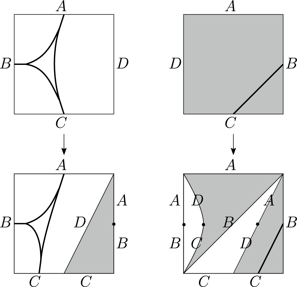
Figure 9 An example of level- $0,1$
non-expanding spines, which are non-essential.
$0,1$
non-expanding spines, which are non-essential.
Definition 6.18. (Nested sequence of non-expanding spines)
For any $n>m\ge 0$
, there is a natural map
$n>m\ge 0$
, there is a natural map $\phi ^n_m:N^n\to N^m$
sending every level-n recurrent bone to its level-m parent. Since
$\phi ^n_m:N^n\to N^m$
sending every level-n recurrent bone to its level-m parent. Since $\mathcal {R}^n(S_{\mathcal {R}})$
is a subdivision of
$\mathcal {R}^n(S_{\mathcal {R}})$
is a subdivision of $\mathcal {R}^m(S_{\mathcal {R}})$
, we may consider
$\mathcal {R}^m(S_{\mathcal {R}})$
, we may consider $N^n$
and
$N^n$
and $N^m$
as train-tracks in the same complex
$N^m$
as train-tracks in the same complex $\mathcal {R}^m(S_{\mathcal {R}})$
. Then the map
$\mathcal {R}^m(S_{\mathcal {R}})$
. Then the map $\phi ^n_m$
is ambient homotopic to the the identity map relative to the
$\phi ^n_m$
is ambient homotopic to the the identity map relative to the $1$
-skeleton
$1$
-skeleton $\mathcal {R}^m(S_{\mathcal {R}})^{(1)}$
of the level-m subdivision complex, that is, there is an extension
$\mathcal {R}^m(S_{\mathcal {R}})^{(1)}$
of the level-m subdivision complex, that is, there is an extension $\phi ^n_m:\mathcal {R}^m(S_{\mathcal {R}})\to \mathcal {R}^m(S_{\mathcal {R}})$
that sends, possibly non-homeomorphically, every edge to the same edge and fixes vertices point-wisely. It is straightforward from definitions that the map
$\phi ^n_m:\mathcal {R}^m(S_{\mathcal {R}})\to \mathcal {R}^m(S_{\mathcal {R}})$
that sends, possibly non-homeomorphically, every edge to the same edge and fixes vertices point-wisely. It is straightforward from definitions that the map $\phi ^n_m:N^n\to N^m$
is a train-track map. Then we have a sequence of train-track maps
$\phi ^n_m:N^n\to N^m$
is a train-track map. Then we have a sequence of train-track maps
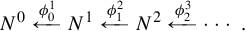 $$ \begin{align*} N^0 \xleftarrow[]{\phi^1_0} N^1 \xleftarrow[]{\phi^2_1} N^2 \xleftarrow[]{\phi^3_2} \cdots. \end{align*} $$
We call this sequence the nested sequence of non-expanding spines.
For example, in Figure 7, each tripod is mapped to a curve by $\phi ^1_0$
and
$\phi ^1_0$
and $\phi ^2_1$
.
$\phi ^2_1$
.
Proposition 6.19. Let $\mathcal {R}$
be a finite subdivision rule and
$\mathcal {R}$
be a finite subdivision rule and $N^n$
be the level-n non-expanding spine of
$N^n$
be the level-n non-expanding spine of $\mathcal {R}$
. For any
$\mathcal {R}$
. For any $n>m$
, if
$n>m$
, if $N^n$
is essential relative to A, then
$N^n$
is essential relative to A, then $N^m$
is also essential relative to A.
$N^m$
is also essential relative to A.
Proof. Since $N^n$
is essential, there is a close curve
$N^n$
is essential, there is a close curve $\gamma $
supported in
$\gamma $
supported in $N^n$
such that
$N^n$
such that $\gamma $
is neither homotopically trivial nor homotopic to some iterates of the peripheral loop of a Julia point in A. Then
$\gamma $
is neither homotopically trivial nor homotopic to some iterates of the peripheral loop of a Julia point in A. Then $\phi ^n_m(\gamma )$
is a closed curve supported in
$\phi ^n_m(\gamma )$
is a closed curve supported in $N^m$
with the same property. Then
$N^m$
with the same property. Then $N^m$
is essential.
$N^m$
is essential.
6.3.1 Restriction of the ranges of non-expanded recurrent curves to
$N^n$

Let $\mathcal {R}$
be a finite subdivision rule. Let
$\mathcal {R}$
be a finite subdivision rule. Let $A\subset \operatorname{Vert}(S_{\mathcal {R}})$
be a set of marked points. It is straightforward from Proposition 6.12 that a closed curve
$A\subset \operatorname{Vert}(S_{\mathcal {R}})$
be a set of marked points. It is straightforward from Proposition 6.12 that a closed curve $\gamma :I\to S^2\setminus A$
is homotopic relative to A to a level-n recurrent non-expanded curve if and only if it is carried by
$\gamma :I\to S^2\setminus A$
is homotopic relative to A to a level-n recurrent non-expanded curve if and only if it is carried by $N^n$
in
$N^n$
in $(S^2,A)$
. Hence, when considering a level-n non-expanded recurrent curve
$(S^2,A)$
. Hence, when considering a level-n non-expanded recurrent curve $\gamma :I\to \mathcal {R}^n(S_{\mathcal {R}})$
, we can restrict the range to
$\gamma :I\to \mathcal {R}^n(S_{\mathcal {R}})$
, we can restrict the range to $N^n \subset \mathcal {R}^n(S_{\mathcal {R}})$
and think of
$N^n \subset \mathcal {R}^n(S_{\mathcal {R}})$
and think of $\gamma $
as a curve supported in
$\gamma $
as a curve supported in $N^n$
.
$N^n$
.
Proposition 6.20. Let $\mathcal {R}$
be a finite subdivision rule and
$\mathcal {R}$
be a finite subdivision rule and ![]() be the subdivision map where
be the subdivision map where $A\subset \operatorname{Vert}(S_{\mathcal {R}})$
is a set of marked points. Let
$A\subset \operatorname{Vert}(S_{\mathcal {R}})$
is a set of marked points. Let $\textrm {ord}:A\to [2,\infty ]_{\mathbb {Z}}$
be a hyperbolic orbisphere structure of
$\textrm {ord}:A\to [2,\infty ]_{\mathbb {Z}}$
be a hyperbolic orbisphere structure of ![]() . Then the level-n non-expanding spine
. Then the level-n non-expanding spine $N^n$
is homotopically infinite for every
$N^n$
is homotopically infinite for every $n\ge 0$
if and only if there is a genealogical sequence of level-n homotopically infinite non-expanded recurrent curves
$n\ge 0$
if and only if there is a genealogical sequence of level-n homotopically infinite non-expanded recurrent curves $\{\gamma ^n:(-\infty ,\infty )\to N^n \subset \mathcal {R}^n(S_{\mathcal {R}})\}_{n \ge 0}$
.
$\{\gamma ^n:(-\infty ,\infty )\to N^n \subset \mathcal {R}^n(S_{\mathcal {R}})\}_{n \ge 0}$
.
Proof. If $N^n$
is not homotopically infinite, then every closed curve is homotopically finite, that is, either trivial or some iterate of the peripheral loop of
$N^n$
is not homotopically infinite, then every closed curve is homotopically finite, that is, either trivial or some iterate of the peripheral loop of $a\in A$
with
$a\in A$
with $\textrm {ord}(a)< \infty $
. Since
$\textrm {ord}(a)< \infty $
. Since $N^n$
consists of finitely many bones, any infinite curve in
$N^n$
consists of finitely many bones, any infinite curve in $N^n$
is approximated by closed curves. Then any infinite curve supported in
$N^n$
is approximated by closed curves. Then any infinite curve supported in $N^n$
also cannot be homotopically infinite, so the desired genealogical sequence of curves does not exist.
$N^n$
also cannot be homotopically infinite, so the desired genealogical sequence of curves does not exist.
Suppose that $N^n$
is homotopically infinite for every
$N^n$
is homotopically infinite for every $n\ge 0$
. We are going to define a set
$n\ge 0$
. We are going to define a set $C^n$
of homotopically infinite non-expanded recurrent curves supported in
$C^n$
of homotopically infinite non-expanded recurrent curves supported in $N^n$
so that the maps
$N^n$
so that the maps $\{\phi ^n_m:C^n\to C^m~|~n>m\ge 0\}$
send any level-n non-expanded recurrent curves to their level-m parents. We will also: (1) define a metric
$\{\phi ^n_m:C^n\to C^m~|~n>m\ge 0\}$
send any level-n non-expanded recurrent curves to their level-m parents. We will also: (1) define a metric $d_n$
on each
$d_n$
on each $C^n$
for which the continuity of
$C^n$
for which the continuity of $\phi ^n_m$
easily follows and (2) show that every
$\phi ^n_m$
easily follows and (2) show that every $C^n$
is compact. Then the inverse limit of
$C^n$
is compact. Then the inverse limit of $\{\phi ^n_m:C^n\to C^m~|~n>m\ge 0\}$
is non-empty whose every element yields a desired genealogical sequence of homotopically infinite non-expanded recurrent curves.
$\{\phi ^n_m:C^n\to C^m~|~n>m\ge 0\}$
is non-empty whose every element yields a desired genealogical sequence of homotopically infinite non-expanded recurrent curves.
Recall that a level-n non-expanded curve $\alpha :(-\infty ,\infty ) \to \mathcal {R}^n(S_{\mathcal {R}})$
is defined to satisfy that for any
$\alpha :(-\infty ,\infty ) \to \mathcal {R}^n(S_{\mathcal {R}})$
is defined to satisfy that for any $n\in \mathbb {Z}$
,
$n\in \mathbb {Z}$
, $\alpha ([n,n+1])$
is a level-n bone. Let us define the set
$\alpha ([n,n+1])$
is a level-n bone. Let us define the set $C^n$
as the collection of (parameterized) level-n homotopically infinite non-expanded recurrent curves
$C^n$
as the collection of (parameterized) level-n homotopically infinite non-expanded recurrent curves $\gamma ^n:(-\infty ,\infty )\to N^n$
up to reparameterization such that
$\gamma ^n:(-\infty ,\infty )\to N^n$
up to reparameterization such that $\gamma ^n$
does not contain a homotopically finite closed curve, which is a closed curve whose free homotopy class corresponds to the conjugate class of a torsion element of
$\gamma ^n$
does not contain a homotopically finite closed curve, which is a closed curve whose free homotopy class corresponds to the conjugate class of a torsion element of $\pi _1(S^2,A,\textrm {ord})$
. Each
$\pi _1(S^2,A,\textrm {ord})$
. Each $C^n$
is non-empty because
$C^n$
is non-empty because $N^n$
is homotopically infinite. We define a metric
$N^n$
is homotopically infinite. We define a metric $d_n$
on
$d_n$
on $C^n$
by
$C^n$
by $d_n(\gamma ^n,\delta ^n)=2^{-m}$
, where
$d_n(\gamma ^n,\delta ^n)=2^{-m}$
, where $\gamma ^n,\delta ^n\in C^n$
and
$\gamma ^n,\delta ^n\in C^n$
and $m>0$
is the minimal integer satisfying
$m>0$
is the minimal integer satisfying $\gamma ^n([-m,m])\neq \delta ^n([-m,m])$
as unions of level-n bones. It is easy to show that for
$\gamma ^n([-m,m])\neq \delta ^n([-m,m])$
as unions of level-n bones. It is easy to show that for $\alpha ^n,\beta ^n,\gamma ^n\in C^n$
,
$\alpha ^n,\beta ^n,\gamma ^n\in C^n$
,
 $$ \begin{align*} d_n(\alpha^n,\gamma^n) = \max( d_n(\alpha^n,\beta^n), d_n(\beta^n,\gamma^n) ), \end{align*} $$
so that $d_n$
is indeed a metric. It is immediate from the definition that
$d_n$
is indeed a metric. It is immediate from the definition that $\phi ^n_m:(C^n,d_n)\to (C^m,d_m)$
is distance non-increasing. Hence,
$\phi ^n_m:(C^n,d_n)\to (C^m,d_m)$
is distance non-increasing. Hence, $\phi ^n_m$
is uniformly continuous.
$\phi ^n_m$
is uniformly continuous.
Lastly, let us show that $(C^n,d_n)$
is sequentially compact. Suppose that
$(C^n,d_n)$
is sequentially compact. Suppose that $\{\gamma ^n_i\in C_n\}_{i\ge 1}$
is any sequence in
$\{\gamma ^n_i\in C_n\}_{i\ge 1}$
is any sequence in $C^n$
. Recall that
$C^n$
. Recall that $\gamma ^n_i([0,1])$
is a bone of level-n band so that, in particular,
$\gamma ^n_i([0,1])$
is a bone of level-n band so that, in particular, $\gamma ^n_i(0)$
is a point in
$\gamma ^n_i(0)$
is a point in $N^n \cap \mathcal {R}^n(S_{\mathcal {R}})^{(1)}$
, which is a finite set. By dropping to a subsequence, we may assume that there exists
$N^n \cap \mathcal {R}^n(S_{\mathcal {R}})^{(1)}$
, which is a finite set. By dropping to a subsequence, we may assume that there exists $x\in N^n$
such that
$x\in N^n$
such that $\gamma ^n_i(0)=x$
for any
$\gamma ^n_i(0)=x$
for any $i>0$
. Let
$i>0$
. Let $p:\mathbb {D} \to S^2 \setminus A^\infty $
be the orbifold universal covering map of
$p:\mathbb {D} \to S^2 \setminus A^\infty $
be the orbifold universal covering map of $(S^2,A,\textrm {ord})$
, where
$(S^2,A,\textrm {ord})$
, where $A^\infty =\{a\in A~|~ \textrm {ord}(a)=\infty \}$
. Choose
$A^\infty =\{a\in A~|~ \textrm {ord}(a)=\infty \}$
. Choose $\widetilde {x} \in p^{-1}(x)$
. For every
$\widetilde {x} \in p^{-1}(x)$
. For every $i>0$
, there exists a unique lifting
$i>0$
, there exists a unique lifting $\widetilde {\gamma }^n_i:(-\infty ,\infty )\to p^{-1}(N^n)$
with
$\widetilde {\gamma }^n_i:(-\infty ,\infty )\to p^{-1}(N^n)$
with $\widetilde {\gamma }^n_i(0)=\widetilde {x}$
. Define
$\widetilde {\gamma }^n_i(0)=\widetilde {x}$
. Define $S_0:=\{\widetilde {\gamma }^n_i\}_{i\ge 1}$
.
$S_0:=\{\widetilde {\gamma }^n_i\}_{i\ge 1}$
.
Fix $r>0$
. Let
$r>0$
. Let $B(\widetilde {x},r)\subset \mathbb {D}$
denote the hyperbolic ball of radius
$B(\widetilde {x},r)\subset \mathbb {D}$
denote the hyperbolic ball of radius $r>0$
with the center at
$r>0$
with the center at $\widetilde {x}$
. For any
$\widetilde {x}$
. For any $i>0$
and some
$i>0$
and some $k_i,l_i\in \mathbb {Z}_{\ge 0}$
, we say that
$k_i,l_i\in \mathbb {Z}_{\ge 0}$
, we say that $\widetilde {\gamma }^n_i([-k_i,l_i])$
is the longest initial subcurve of
$\widetilde {\gamma }^n_i([-k_i,l_i])$
is the longest initial subcurve of $\widetilde {\gamma }^n_i$
staying in
$\widetilde {\gamma }^n_i$
staying in $B(\widetilde {x},r)$
if
$B(\widetilde {x},r)$
if $\widetilde {\gamma }^n_i([-k_i,l_i])\subset B(\widetilde {x},r)$
and
$\widetilde {\gamma }^n_i([-k_i,l_i])\subset B(\widetilde {x},r)$
and $\widetilde {\gamma }^n_i(-k_i-1), \widetilde {\gamma }^n_i(l_i+1) \notin B(\widetilde {x},r)$
. The intersection
$\widetilde {\gamma }^n_i(-k_i-1), \widetilde {\gamma }^n_i(l_i+1) \notin B(\widetilde {x},r)$
. The intersection $B(\widetilde {x},r)\cap p^{-1}(N^n)$
has at most finitely many edges of
$B(\widetilde {x},r)\cap p^{-1}(N^n)$
has at most finitely many edges of $p^{-1}(N^n)$
. Since every element of
$p^{-1}(N^n)$
. Since every element of $C^n$
does not contain a homotopically finite closed curve, any
$C^n$
does not contain a homotopically finite closed curve, any $\widetilde {\gamma }^n_i$
does not contain a closed curve. It follows that there exists
$\widetilde {\gamma }^n_i$
does not contain a closed curve. It follows that there exists $m_1<m_2<\cdots $
such that every element of the subsequence
$m_1<m_2<\cdots $
such that every element of the subsequence $\{\widetilde {\gamma }^n_{m_i}\}_{i>0}$
of
$\{\widetilde {\gamma }^n_{m_i}\}_{i>0}$
of $S_0$
has the same longest initial subcurve staying in
$S_0$
has the same longest initial subcurve staying in $B(\widetilde {x},r)$
.
$B(\widetilde {x},r)$
.
Take a sequence $0<r_1<r_2<\cdots $
with
$0<r_1<r_2<\cdots $
with $r_i\to \infty $
. For any
$r_i\to \infty $
. For any $m>0$
, define
$m>0$
, define $S_m$
as a subsequence of
$S_m$
as a subsequence of $S_{m-1}$
whose elements have the same longest initial subcurve staying in
$S_{m-1}$
whose elements have the same longest initial subcurve staying in $B(\widetilde {x},r_m)$
. By taking the diagonal of a sequence of subsequences
$B(\widetilde {x},r_m)$
. By taking the diagonal of a sequence of subsequences $S_0,S_1,S_2,\ldots $
, we have a subsequence
$S_0,S_1,S_2,\ldots $
, we have a subsequence $\{\widetilde {\gamma }^n_{m_i}\}$
of
$\{\widetilde {\gamma }^n_{m_i}\}$
of $S_0$
with the following property. There exist two strictly increasing sequences of positive integers
$S_0$
with the following property. There exist two strictly increasing sequences of positive integers $\{a_i\}_{i\ge 0}$
and
$\{a_i\}_{i\ge 0}$
and $\{b_i\}_{i\ge 0}$
such that:
$\{b_i\}_{i\ge 0}$
such that:
-
(1)
$\widetilde {\gamma }^n_{m_i}([-a_i,b_i])$
is the longest initial subcurve staying in
$B(\widetilde {x},r_i)$
and -
(2)
$\widetilde {\gamma }^n_{m_j}([-a_i,b_i])=\widetilde {\gamma }^n_{m_i}([-a_i,b_i])$
for any
$j>i$
, that is, the initial subcurves are accumulated.


We define a curve $\widetilde {\gamma }^n:(-\infty ,\infty )\to p^{-1}(N^n)$
by
$\widetilde {\gamma }^n:(-\infty ,\infty )\to p^{-1}(N^n)$
by $\widetilde {\gamma }^n|_{[-a_i,b_i]}=\widetilde {\gamma }^n_i|_{[-a_i,b_i]}$
for every
$\widetilde {\gamma }^n|_{[-a_i,b_i]}=\widetilde {\gamma }^n_i|_{[-a_i,b_i]}$
for every $i\ge 1$
, which is well defined by property (2). It follows from property (1) that for any
$i\ge 1$
, which is well defined by property (2). It follows from property (1) that for any $i\ge 1$
, we have
$i\ge 1$
, we have
 $$ \begin{align*} d_{\mathbb{D}}(\widetilde{x},\widetilde{\gamma}^n(-a_i-1)),~d_{\mathbb{D}}(\widetilde{x},\widetilde{\gamma}^n(b_i+1))>r_i, \end{align*} $$
where $d_{\mathbb {D}}$
is the hyperbolic metric on
$d_{\mathbb {D}}$
is the hyperbolic metric on $\mathbb {D}$
. Hence,
$\mathbb {D}$
. Hence, $\gamma ^n:=p \circ \widetilde {\gamma }^n$
is homotopically infinite. Then
$\gamma ^n:=p \circ \widetilde {\gamma }^n$
is homotopically infinite. Then $\gamma ^n_{m_i}\to \gamma ^n\in C^n$
, which implies
$\gamma ^n_{m_i}\to \gamma ^n\in C^n$
, which implies $(C^n,d_n)$
is sequentially compact.
$(C^n,d_n)$
is sequentially compact.
Theorem 6.21. Let $\mathcal {R}$
be a finite subdivision rule and
$\mathcal {R}$
be a finite subdivision rule and $f:\mathcal {R}(S_{\mathcal {R}})\to S_{\mathcal {R}}$
be its subdivision map which is not doubly covered by a torus endomorphism. Let
$f:\mathcal {R}(S_{\mathcal {R}})\to S_{\mathcal {R}}$
be its subdivision map which is not doubly covered by a torus endomorphism. Let $A\subset \operatorname{Vert}(S_{\mathcal {R}})$
be a set of marked points, that is,
$A\subset \operatorname{Vert}(S_{\mathcal {R}})$
be a set of marked points, that is, $P_f \cup f(A)\subset A$
. Then the post-critically finite branched covering
$P_f \cup f(A)\subset A$
. Then the post-critically finite branched covering ![]() has a Levy cycle if and only if the level-n non-expanding spine
has a Levy cycle if and only if the level-n non-expanding spine $N^n$
is essential relative to A for every
$N^n$
is essential relative to A for every $n\ge 0$
.
$n\ge 0$
.
Proof. Let $\textrm {ord}:A\to [2,\infty ]_{\mathbb {Z}}$
be an orbisphere structure. Any multiplication of
$\textrm {ord}:A\to [2,\infty ]_{\mathbb {Z}}$
be an orbisphere structure. Any multiplication of $\textrm {ord}$
by a positive integer gives rise to another orbisphere structure with strictly decreased Euler characteristic. Similarly, changing the order of every Fatou point in A into infinity also yields an orbisphere structure with strictly decreased Euler characteristic, if some order was actually changed. Hence, we always have a hyperbolic orbisphere structure
$\textrm {ord}$
by a positive integer gives rise to another orbisphere structure with strictly decreased Euler characteristic. Similarly, changing the order of every Fatou point in A into infinity also yields an orbisphere structure with strictly decreased Euler characteristic, if some order was actually changed. Hence, we always have a hyperbolic orbisphere structure $\textrm {ord}:A\to [2,\infty ]_{\mathbb {Z}}$
with the property that
$\textrm {ord}:A\to [2,\infty ]_{\mathbb {Z}}$
with the property that $\textrm {ord}(a)=\infty $
if and only if
$\textrm {ord}(a)=\infty $
if and only if $a\in A$
is a Fatou point. Then a closed curve is homotopically infinite with respect to
$a\in A$
is a Fatou point. Then a closed curve is homotopically infinite with respect to $\textrm {ord}$
if and only if it is neither homotopic relative to A to a point nor to some iterate of a peripheral loop of a Julia point in A. Then the theorem follows from Propositions 5.14, 5.15, and 6.20.
$\textrm {ord}$
if and only if it is neither homotopic relative to A to a point nor to some iterate of a peripheral loop of a Julia point in A. Then the theorem follows from Propositions 5.14, 5.15, and 6.20.
7 Graph intersecting obstruction
7.1 Graph intersecting obstructions
Suppose that ![]() is a post-critically finite branched covering. A graph
is a post-critically finite branched covering. A graph $G\subset S^2$
is forward invariant under f up to isotopy relative to A if there exist a subgraph H of
$G\subset S^2$
is forward invariant under f up to isotopy relative to A if there exist a subgraph H of $f^{-1}(G)$
and a homeomorphism
$f^{-1}(G)$
and a homeomorphism $\phi :S^2\to S^2$
such that
$\phi :S^2\to S^2$
such that $\phi (H)=G$
and
$\phi (H)=G$
and $\phi $
is isotopic to the identity map relative to A. A graph G is forward invariant under f if
$\phi $
is isotopic to the identity map relative to A. A graph G is forward invariant under f if $f(G)\subset G$
. A multicurve
$f(G)\subset G$
. A multicurve $\Gamma $
on
$\Gamma $
on $(S^2,A)$
is forward invariant under f up to isotopy relative to A if it is so as a graph. A multicurve
$(S^2,A)$
is forward invariant under f up to isotopy relative to A if it is so as a graph. A multicurve $\Gamma $
is backward invariant under f up to isotopy relative to A, or f-stable, if every connected component of
$\Gamma $
is backward invariant under f up to isotopy relative to A, or f-stable, if every connected component of $f^{-1}(\gamma )$
for
$f^{-1}(\gamma )$
for $\gamma \in \Gamma $
is either isotopic relative to A to an element of
$\gamma \in \Gamma $
is either isotopic relative to A to an element of $\Gamma $
or peripheral to A. When f and A are understood, we omit ‘under f’ and ‘relative to A’.
$\Gamma $
or peripheral to A. When f and A are understood, we omit ‘under f’ and ‘relative to A’.
Proposition 7.1. Let ![]() be a post-critically finite branched covering and G be a graph that is forward invariant up to isotopy. Then there exists
be a post-critically finite branched covering and G be a graph that is forward invariant up to isotopy. Then there exists ![]() which is isotopic to
which is isotopic to ![]() relative to A, such that G is forward invariant under a post-critically finite branched covering
relative to A, such that G is forward invariant under a post-critically finite branched covering ![]() defined by
defined by $g:=f \circ \iota $
. Especially, f and g are combinatorially equivalent by
$g:=f \circ \iota $
. Especially, f and g are combinatorially equivalent by $\textrm {id}_{S^2}$
and
$\textrm {id}_{S^2}$
and $\iota $
.
$\iota $
.
Proof. Let H be a subgraph of $f^{-1}(G)$
isotopic to G rel
$f^{-1}(G)$
isotopic to G rel $\operatorname{Vert}(G)$
. By extending the isotopy to
$\operatorname{Vert}(G)$
. By extending the isotopy to $S^2$
, we have
$S^2$
, we have $\iota :(S^2,A) \to (S^2,A)$
such that
$\iota :(S^2,A) \to (S^2,A)$
such that $\iota (G)=H$
, and
$\iota (G)=H$
, and $\iota $
and
$\iota $
and $\textrm {id}_{S^2}$
are isotopic relative to A. Let
$\textrm {id}_{S^2}$
are isotopic relative to A. Let $g:=f \circ \iota $
. Then
$g:=f \circ \iota $
. Then $\textrm {id} \circ g=f \circ \iota $
and
$\textrm {id} \circ g=f \circ \iota $
and $g(G)=f(\iota (G))=f(H) \subset G$
.
$g(G)=f(\iota (G))=f(H) \subset G$
.
Due to Proposition 7.1, we may consider forward invariant graphs instead of graphs that are forward invariant up to isotopy when discussing properties of combinatorial equivalence classes, such as Levy cycles and Thurston obstructions.
Let $\Gamma $
be a multicurve in
$\Gamma $
be a multicurve in $S^2 \setminus A$
. The Thurston linear transformation of
$S^2 \setminus A$
. The Thurston linear transformation of $\Gamma $
is a linear map
$\Gamma $
is a linear map $f_\Gamma :\mathbb {R}^\Gamma \to \mathbb {R}^\Gamma $
defined by
$f_\Gamma :\mathbb {R}^\Gamma \to \mathbb {R}^\Gamma $
defined by
 $$ \begin{align*} f_\Gamma (\gamma)=\sum\limits_{\gamma'\subset f^{-1}(\gamma)}\frac{1}{\deg (f|_{\gamma'}:\gamma' \to \gamma)} [\gamma']_\Gamma, \end{align*} $$
where $\gamma '$
is a connected component of
$\gamma '$
is a connected component of $f^{-1}(\gamma )$
and
$f^{-1}(\gamma )$
and $[\gamma ']_\Gamma $
is an element of
$[\gamma ']_\Gamma $
is an element of $\Gamma $
isotopic to
$\Gamma $
isotopic to $\gamma '$
if it exists. If no such connected component exists, then the sum is defined to be zero. Since
$\gamma '$
if it exists. If no such connected component exists, then the sum is defined to be zero. Since $f_\Gamma $
is a non-negative matrix, it has a non-negative real eigenvalue
$f_\Gamma $
is a non-negative matrix, it has a non-negative real eigenvalue $\unicode{x3bb} (f_\Gamma )$
that is the spectral radius of
$\unicode{x3bb} (f_\Gamma )$
that is the spectral radius of $f_\Gamma $
. If
$f_\Gamma $
. If $\unicode{x3bb} (f_\Gamma )\ge 1$
, then
$\unicode{x3bb} (f_\Gamma )\ge 1$
, then $\Gamma $
is a Thurston obstruction. An
$\Gamma $
is a Thurston obstruction. An $n\times n$
non-negative square matrix M is irreducible if for each
$n\times n$
non-negative square matrix M is irreducible if for each $i,\,j$
with
$i,\,j$
with $1 \le i,\,j\le n$
, there exists
$1 \le i,\,j\le n$
, there exists $k\ge 1$
such that the
$k\ge 1$
such that the $(i,\,j)$
-entry of
$(i,\,j)$
-entry of $M^k$
is positive. An irreducible multicurve
$M^k$
is positive. An irreducible multicurve $\Gamma $
is a multicurve whose Thurston linear transformation
$\Gamma $
is a multicurve whose Thurston linear transformation $f_\Gamma $
is irreducible. An irreducible Thurston obstruction is an irreducible multicurve that is a Thurston obstruction.
$f_\Gamma $
is irreducible. An irreducible Thurston obstruction is an irreducible multicurve that is a Thurston obstruction.
Remark 7.2. A Thurston obstruction $\Gamma $
is usually assumed to be f-stable. For any multicurve
$\Gamma $
is usually assumed to be f-stable. For any multicurve $\Gamma $
with
$\Gamma $
with $\unicode{x3bb} (f_\Gamma )\neq 0$
, there exists a sub-multicurve
$\unicode{x3bb} (f_\Gamma )\neq 0$
, there exists a sub-multicurve $\Gamma ' \subset \Gamma $
such that
$\Gamma ' \subset \Gamma $
such that $\Gamma '$
is irreducible and
$\Gamma '$
is irreducible and $\unicode{x3bb} (f_{\Gamma '})=\unicode{x3bb} (f_\Gamma )$
. Such
$\unicode{x3bb} (f_{\Gamma '})=\unicode{x3bb} (f_\Gamma )$
. Such $\Gamma '$
is determined as the multicurve of an irreducible diagonal block
$\Gamma '$
is determined as the multicurve of an irreducible diagonal block $A_i$
of the upper-triangular block form in equation (UTB-form) of
$A_i$
of the upper-triangular block form in equation (UTB-form) of $f_\Gamma $
with
$f_\Gamma $
with $\unicode{x3bb} (A_i)=\unicode{x3bb} (f_\Gamma )$
. By Lemma 7.4,
$\unicode{x3bb} (A_i)=\unicode{x3bb} (f_\Gamma )$
. By Lemma 7.4, $\Gamma '$
extends to an f-invariant multicurve
$\Gamma '$
extends to an f-invariant multicurve $\Gamma "$
with
$\Gamma "$
with $\unicode{x3bb} (f_{\Gamma "})\ge \unicode{x3bb} (f_{\Gamma })$
. Hence, we may drop the f-condition condition from Thurston’s characterization.
$\unicode{x3bb} (f_{\Gamma "})\ge \unicode{x3bb} (f_{\Gamma })$
. Hence, we may drop the f-condition condition from Thurston’s characterization.
Lemma 7.3. If a multicurve $\Gamma $
is irreducible, then
$\Gamma $
is irreducible, then $\Gamma $
is forward invariant up to isotopy.
$\Gamma $
is forward invariant up to isotopy.
Proof. For a contradiction, assume there exists $\gamma $
such that for every
$\gamma $
such that for every $\gamma '\in \Gamma $
, no connected component of
$\gamma '\in \Gamma $
, no connected component of $f^{-1}(\gamma ')$
is isotopic to
$f^{-1}(\gamma ')$
is isotopic to $\gamma $
. Then
$\gamma $
. Then $f_\Gamma :\mathbb {R}^\Gamma \to \mathbb {R}^{\Gamma \setminus \{\gamma \}} \subset \mathbb {R}^{\Gamma }$
, and thus
$f_\Gamma :\mathbb {R}^\Gamma \to \mathbb {R}^{\Gamma \setminus \{\gamma \}} \subset \mathbb {R}^{\Gamma }$
, and thus $f_\Gamma $
is not irreducible.
$f_\Gamma $
is not irreducible.
Lemma 7.4. [Reference TanTan92, Lemma 2.2]
For any multicurve $\Gamma $
of
$\Gamma $
of $(S^2,A)$
that is forward invariant up to isotopy, there exists a multicurve
$(S^2,A)$
that is forward invariant up to isotopy, there exists a multicurve $\Gamma '$
which is backward invariant up to isotopy such that
$\Gamma '$
which is backward invariant up to isotopy such that $\Gamma ' \supset \Gamma $
and
$\Gamma ' \supset \Gamma $
and $\unicode{x3bb} (f_{\Gamma '}) \ge \unicode{x3bb} (f_{\Gamma })$
.
$\unicode{x3bb} (f_{\Gamma '}) \ge \unicode{x3bb} (f_{\Gamma })$
.
Proof. Let $\Gamma _0=\Gamma $
and
$\Gamma _0=\Gamma $
and $\Gamma _n$
be the set of homotopy classes of essential curves in
$\Gamma _n$
be the set of homotopy classes of essential curves in $f^{-n}(\Gamma _0)$
. By the forward invariance up to isotopy,
$f^{-n}(\Gamma _0)$
. By the forward invariance up to isotopy, $\Gamma _0 \subset \Gamma _1 \subset \cdots $
is an increasing sequence of multicurves. Note that
$\Gamma _0 \subset \Gamma _1 \subset \cdots $
is an increasing sequence of multicurves. Note that $|A|-3$
is the maximal number of non-homotopic essential simple closed curves that can be disjointly embedded into
$|A|-3$
is the maximal number of non-homotopic essential simple closed curves that can be disjointly embedded into $S^2\setminus A$
. Hence, there exists n such that
$S^2\setminus A$
. Hence, there exists n such that $\Gamma _n$
is f-invariant. The inequality
$\Gamma _n$
is f-invariant. The inequality $\unicode{x3bb} (f_{\Gamma '}) \ge \unicode{x3bb} (f_{\Gamma })$
follows from the following: for non-negative square matrices M and N, if
$\unicode{x3bb} (f_{\Gamma '}) \ge \unicode{x3bb} (f_{\Gamma })$
follows from the following: for non-negative square matrices M and N, if $M_{ij} \ge N_{ij}$
for every
$M_{ij} \ge N_{ij}$
for every $(i,\,j)$
, then
$(i,\,j)$
, then $\unicode{x3bb} (M) \ge \unicode{x3bb} (N)$
.
$\unicode{x3bb} (M) \ge \unicode{x3bb} (N)$
.
Theorem 7.5. (Arcs intersecting obstructions [Reference Pilgrim and TanPT98, Theorem 3.2])
Let ![]() be a post-critically finite branched covering and G be an invariant graph such that
be a post-critically finite branched covering and G be an invariant graph such that $f|_G:G \to G$
is a graph automorphism. Then every irreducible Thurston obstruction intersecting G is a Levy cycle.
$f|_G:G \to G$
is a graph automorphism. Then every irreducible Thurston obstruction intersecting G is a Levy cycle.
We generalize it to a case when G is an f-invariant graph with $h_{\textrm {top}}(f|_G)=0$
.
$h_{\textrm {top}}(f|_G)=0$
.
Theorem 7.6. (Graph intersecting obstruction)
Let ![]() be a post-critically finite branched covering and G be a forward invariant graph such that
be a post-critically finite branched covering and G be a forward invariant graph such that $h_{\textrm {top}}(f|_G)=0$
. Then every irreducible Thurston obstruction intersecting G is a Levy cycle.
$h_{\textrm {top}}(f|_G)=0$
. Then every irreducible Thurston obstruction intersecting G is a Levy cycle.
Remark 7.7. The graphs in Theorems 7.5 and 7.6 are possibly disconnected. Moreover, the same statement works for graphs which are forward invariant up to isotopy by Proposition 7.1 with a slight modification to define $h_{\textrm {top}}(f|_G)$
.
$h_{\textrm {top}}(f|_G)$
.
An arc of $(S^2,A)$
is a curve embedded in
$(S^2,A)$
is a curve embedded in $S^2$
such that its interior is embedded in
$S^2$
such that its interior is embedded in $S^2 \setminus A$
and its endpoints are in A. A geometric intersection number
$S^2 \setminus A$
and its endpoints are in A. A geometric intersection number $\gamma \cdot \gamma '$
between curves (arcs and simple closed curves) is defined as the minimal number of intersection points in their isotopy classes relative to A.
$\gamma \cdot \gamma '$
between curves (arcs and simple closed curves) is defined as the minimal number of intersection points in their isotopy classes relative to A.
For a multicurve $\Gamma $
, the unweighted Thurston transformation
$\Gamma $
, the unweighted Thurston transformation $f_{\#,\Gamma }:\mathbb {R}^\Gamma \to \mathbb {R}^\Gamma $
is defined by
$f_{\#,\Gamma }:\mathbb {R}^\Gamma \to \mathbb {R}^\Gamma $
is defined by
 $$ \begin{align*} f_{\#,\Gamma}(\gamma)=\sum\limits_{\gamma'\subset f^{-1}(\gamma)} [\gamma']_\Gamma, \end{align*} $$
where $\gamma '$
is a connected component of
$\gamma '$
is a connected component of $f^{-1}(\gamma )$
and
$f^{-1}(\gamma )$
and $[\gamma ']_\Gamma $
is an element of
$[\gamma ']_\Gamma $
is an element of $\Gamma $
isotopic to
$\Gamma $
isotopic to $\gamma '$
if it exists. If there is no such element, then the sum is defined to be zero. For every
$\gamma '$
if it exists. If there is no such element, then the sum is defined to be zero. For every $(i,\,j)$
, (1)
$(i,\,j)$
, (1) $0 \le (f_\Gamma )_{ij} \le (f_{\#,\Gamma })_{ij}$
and (2)
$0 \le (f_\Gamma )_{ij} \le (f_{\#,\Gamma })_{ij}$
and (2) $(f_\Gamma )_{ij}=0$
if and only if
$(f_\Gamma )_{ij}=0$
if and only if $(f_{\#,\Gamma })_{ij}=0$
. So
$(f_{\#,\Gamma })_{ij}=0$
. So $f_{\#,\Gamma }$
is irreducible if and only if
$f_{\#,\Gamma }$
is irreducible if and only if $f_\Gamma $
is irreducible.
$f_\Gamma $
is irreducible.
Proof of Theorem 7.6
Let $\textrm {Edge}(G)=\{e_1,e_2,\ldots ,e_n\}$
. For any simple closed curve
$\textrm {Edge}(G)=\{e_1,e_2,\ldots ,e_n\}$
. For any simple closed curve $\gamma \subset S^2 \setminus A$
, define
$\gamma \subset S^2 \setminus A$
, define
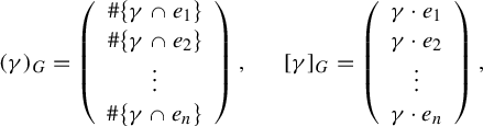 $$ \begin{align*} (\gamma)_G=\left(\begin{array}{c}\# \{\gamma \cap e_1\} \\ \# \{\gamma \cap e_2\} \\ \vdots \\ \# \{\gamma \cap e_n\} \end{array}\right), ~~~~~~ [\gamma]_G= \left( \begin{array}{c}\gamma \cdot e_1 \\ \gamma \cdot e_2 \\ \vdots \\ \gamma \cdot e_n \end{array}\right), \end{align*} $$
where $\gamma \cdot e_i$
means the geometric intersection number of
$\gamma \cdot e_i$
means the geometric intersection number of $\gamma $
and
$\gamma $
and $e_i$
relative to A. The
$e_i$
relative to A. The $(~)_G$
and
$(~)_G$
and $[~]_G$
are linearly extended to weighted multicurves. Let
$[~]_G$
are linearly extended to weighted multicurves. Let $T_G$
be the incidence matrix of
$T_G$
be the incidence matrix of $f|_G$
. Let
$f|_G$
. Let $\Gamma =\{\gamma _1,\gamma _2,\ldots ,\gamma _m\}$
be an irreducible Thurston obstruction. From
$\Gamma =\{\gamma _1,\gamma _2,\ldots ,\gamma _m\}$
be an irreducible Thurston obstruction. From $\# \{f^{-k}(\gamma _i) \cap e_j\} \ge f^{-k}(\gamma _i) \cdot e_j$
, for every
$\# \{f^{-k}(\gamma _i) \cap e_j\} \ge f^{-k}(\gamma _i) \cdot e_j$
, for every $k\ge 1$
, we have
$k\ge 1$
, we have
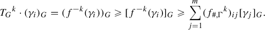 $$ \begin{align} {T_G}^k \cdot (\gamma_i)_G = (f^{-k}(\gamma_i))_G \ge [f^{-k}(\gamma_i)]_G \ge \sum_{j=1}^m({f_{\#,\Gamma}}^k)_{ij}[\gamma_j]_G. \end{align} $$
The third term counts the intersection of G with all connected components of $f^{-k}(\gamma _i)$
, but the last term counts the intersection of G with connected components of
$f^{-k}(\gamma _i)$
, but the last term counts the intersection of G with connected components of $f^{-k}(\gamma _i)$
isotopic relative to A to some connected components of
$f^{-k}(\gamma _i)$
isotopic relative to A to some connected components of $\Gamma $
.
$\Gamma $
.
It follows from Proposition 3.9 that entries of ${T_G}^k$
grow at most polynomially fast, so
${T_G}^k$
grow at most polynomially fast, so $(f_{\#,\Gamma }^k)_{ij}$
grows at most polynomially fast too. Since
$(f_{\#,\Gamma }^k)_{ij}$
grows at most polynomially fast too. Since $f_{\#,\Gamma }$
is an irreducible non-negative integer matrix,
$f_{\#,\Gamma }$
is an irreducible non-negative integer matrix, $f_{\#,\Gamma }$
is a permutation by Lemma 3.8. Recall that: (1)
$f_{\#,\Gamma }$
is a permutation by Lemma 3.8. Recall that: (1) $0 \le (f_\Gamma )_{ij} \le (f_{\#,\Gamma })_{ij}$
and (2)
$0 \le (f_\Gamma )_{ij} \le (f_{\#,\Gamma })_{ij}$
and (2) $(f_\Gamma )_{ij}>0$
if and only if
$(f_\Gamma )_{ij}>0$
if and only if $(f_{\#,\Gamma })_{ij}>0$
. Hence, the only way to have
$(f_{\#,\Gamma })_{ij}>0$
. Hence, the only way to have $\unicode{x3bb} (f_\Gamma ) \ge 1$
is
$\unicode{x3bb} (f_\Gamma ) \ge 1$
is $f_{\#,\Gamma }=f_\Gamma $
. Then
$f_{\#,\Gamma }=f_\Gamma $
. Then $\Gamma $
is a Levy cycle.
$\Gamma $
is a Levy cycle.
7.2 Application in the mating of polynomials
7.2.1 Formal mating
Let f and g be post-critically finite polynomials of degree d. Consider f and g as maps from the complex plane $\mathbb {C}$
to itself. Let
$\mathbb {C}$
to itself. Let $\overline {\mathbb {C}}$
be the compactification of
$\overline {\mathbb {C}}$
be the compactification of $\mathbb {C}$
by the circle
$\mathbb {C}$
by the circle $S^1$
each point of which corresponds to a linear direction to infinity. Then, f and g extend to the boundary
$S^1$
each point of which corresponds to a linear direction to infinity. Then, f and g extend to the boundary $S^1$
as the angle d-times map. We can parameterize
$S^1$
as the angle d-times map. We can parameterize $S^1$
by
$S^1$
by $\theta \in [0,1]/\{0\sim 1\}$
, where
$\theta \in [0,1]/\{0\sim 1\}$
, where $\theta $
indicates the angle of an external ray. Let us use subscriptions
$\theta $
indicates the angle of an external ray. Let us use subscriptions $-_f$
and
$-_f$
and $-_g$
to distinguish two compactified complex planes on which f and g act, respectively, such as
$-_g$
to distinguish two compactified complex planes on which f and g act, respectively, such as $\overline {\mathbb {D}}_f:=\mathbb {C}_f \cup S^1_f$
,
$\overline {\mathbb {D}}_f:=\mathbb {C}_f \cup S^1_f$
, $\overline {\mathbb {D}}_g:=\mathbb {C}_g \cup S^1_g$
,
$\overline {\mathbb {D}}_g:=\mathbb {C}_g \cup S^1_g$
, ![]() and
and ![]() . Define a sphere
. Define a sphere $S^2_{f\uplus g}$
by gluing two compactified planes
$S^2_{f\uplus g}$
by gluing two compactified planes $\overline {\mathbb {C}}_f$
and
$\overline {\mathbb {C}}_f$
and $\overline {\mathbb {C}}_g$
by the equivalence relation
$\overline {\mathbb {C}}_g$
by the equivalence relation $\theta _f\sim -\theta _g$
for any
$\theta _f\sim -\theta _g$
for any $\theta _f\in S^1_f$
and
$\theta _f\in S^1_f$
and $\theta _g\in S^1_g$
with
$\theta _g\in S^1_g$
with $\theta _f=\theta _g$
as numbers in
$\theta _f=\theta _g$
as numbers in $[0,1)$
. The dynamics of f and g also glue together to induce a dynamic
$[0,1)$
. The dynamics of f and g also glue together to induce a dynamic ![]() , which is also a post-critically finite branched self-covering of the sphere. We call
, which is also a post-critically finite branched self-covering of the sphere. We call ![]() the formal mating of f and g.
the formal mating of f and g.
7.2.2 Ray-equivalence class
Let ![]() be the formal mating of post-critically finite polynomials f and g. External rays of f and g form a foliation on
be the formal mating of post-critically finite polynomials f and g. External rays of f and g form a foliation on $S^2_{f\uplus g} \setminus (K_f \cup K_g)$
, where
$S^2_{f\uplus g} \setminus (K_f \cup K_g)$
, where $K_f \subset \mathbb {C}_f$
and
$K_f \subset \mathbb {C}_f$
and $K_f \subset \mathbb {C}_g$
are filled Julia sets. Every leaf of the foliation is called a ray-equivalence class of the formal mating
$K_f \subset \mathbb {C}_g$
are filled Julia sets. Every leaf of the foliation is called a ray-equivalence class of the formal mating $f \uplus g$
. Each ray-equivalence class consists of external rays of f and g of the same period and preperiod.
$f \uplus g$
. Each ray-equivalence class consists of external rays of f and g of the same period and preperiod.
7.2.3 Degenerate mating
If f or g (or both) is non-hyperbolic, there could be an obvious Levy cycle of $f \uplus g$
which could be removed by collapsing some ray equivalence classes.
$f \uplus g$
which could be removed by collapsing some ray equivalence classes.
Let $F:=f \uplus g$
. Suppose that f is not hyperbolic. Then the post-critical set
$F:=f \uplus g$
. Suppose that f is not hyperbolic. Then the post-critical set $P_f$
is in the Julia set
$P_f$
is in the Julia set $\mathcal {J}_f$
so that each post-critical point of f is contained in a ray-equivalence class. Suppose that there is a periodic ray-equivalence class
$\mathcal {J}_f$
so that each post-critical point of f is contained in a ray-equivalence class. Suppose that there is a periodic ray-equivalence class $\xi $
that contains two points of
$\xi $
that contains two points of $P_F$
such that
$P_F$
such that $\xi $
is topologically a tree. Then the boundary of a small neighborhood of
$\xi $
is topologically a tree. Then the boundary of a small neighborhood of $\xi $
generates a Levy cycle. Hence, we will collapse
$\xi $
generates a Levy cycle. Hence, we will collapse $\xi $
to a point. To obtain a topological branched covering on the quotient sphere, we need a little more careful construction as follows, see [Reference Shishikura and LeiShi00] for details.
$\xi $
to a point. To obtain a topological branched covering on the quotient sphere, we need a little more careful construction as follows, see [Reference Shishikura and LeiShi00] for details.
Let $Y'$
be the set of ray-equivalence classes containing at least to points in
$Y'$
be the set of ray-equivalence classes containing at least to points in $\Omega _F \cup P_F$
. Define Y to be the set of ray-equivalence class
$\Omega _F \cup P_F$
. Define Y to be the set of ray-equivalence class $\xi '$
containing at least one point of
$\xi '$
containing at least one point of $\Omega _F \cup P_F$
such that
$\Omega _F \cup P_F$
such that $F^m(\xi ')=F^n(\xi )$
for some
$F^m(\xi ')=F^n(\xi )$
for some $m,n\ge 0$
and
$m,n\ge 0$
and $\xi \in Y$
. If
$\xi \in Y$
. If $Y \neq \emptyset $
and every element of Y is topologically a tree, then we define
$Y \neq \emptyset $
and every element of Y is topologically a tree, then we define $S^{\prime 2}$
as the quotient of
$S^{\prime 2}$
as the quotient of $S^2_{f \uplus g}$
by collapsing every ray-equivalence class in Y to a point. The map F induces a degree d self-map on
$S^2_{f \uplus g}$
by collapsing every ray-equivalence class in Y to a point. The map F induces a degree d self-map on $S^{\prime 2}$
which is not a branched covering near
$S^{\prime 2}$
which is not a branched covering near $F^{-1}(\xi )$
for
$F^{-1}(\xi )$
for $\xi \in Y$
. However, we can take a homotopy near
$\xi \in Y$
. However, we can take a homotopy near $F^{-1}(\xi )$
for
$F^{-1}(\xi )$
for $\xi \in Y$
to obtain a branched covering
$\xi \in Y$
to obtain a branched covering ![]() , which is called the degenerate mating of f and g. We also denote the degenerate mating by
, which is called the degenerate mating of f and g. We also denote the degenerate mating by ![]() . When both f and g are hyperbolic, the degenerate mating is equal to the formal mating.
. When both f and g are hyperbolic, the degenerate mating is equal to the formal mating.
Example 7.8. (
$f_{1/2} \uplus ' f_{1/4}$
)

For $\theta \in \mathbb {Q} \cap [0,1)$
, let
$\theta \in \mathbb {Q} \cap [0,1)$
, let $f_{\theta }$
denote the post-critically finite polynomial at the landing point of the external ray of angle
$f_{\theta }$
denote the post-critically finite polynomial at the landing point of the external ray of angle $\theta $
in the parameter plane of the quadratic polynomials
$\theta $
in the parameter plane of the quadratic polynomials $z^2+c$
. Let
$z^2+c$
. Let $f=f_{1/2}$
and
$f=f_{1/2}$
and $g=f_{1/4}$
. Let us denote by
$g=f_{1/4}$
. Let us denote by $R_f(\theta )$
and
$R_f(\theta )$
and $R_g(\theta )$
the external rays of f and g of angle
$R_g(\theta )$
the external rays of f and g of angle $\theta $
.
$\theta $
.
The set $Y'$
defined above consists of three ray-equivalence classes:
$Y'$
defined above consists of three ray-equivalence classes: $\xi _0:=R_f(0) \cup R_g(0)$
,
$\xi _0:=R_f(0) \cup R_g(0)$
, $\xi _1:=R_f(1/2)\cup R_g(1/2)$
, and
$\xi _1:=R_f(1/2)\cup R_g(1/2)$
, and $\xi _2:=R_f(1/4)\cup R_f(3/4) \cup R_g(1/4) \cup R_g(3/4)$
. The set Y has one more ray-equivalence class
$\xi _2:=R_f(1/4)\cup R_f(3/4) \cup R_g(1/4) \cup R_g(3/4)$
. The set Y has one more ray-equivalence class $\xi _3:=R_f(3/8) \cup R_f(7/8) \cup R_g(1/8)\cup R_g(5/8)$
than
$\xi _3:=R_f(3/8) \cup R_f(7/8) \cup R_g(1/8)\cup R_g(5/8)$
than $Y'$
.
$Y'$
.
Let $F=f \uplus g$
be the formal mating. The boundary of a small disk neighborhood of
$F=f \uplus g$
be the formal mating. The boundary of a small disk neighborhood of $\xi _0$
is a Levy cycle of period one. Let us also use
$\xi _0$
is a Levy cycle of period one. Let us also use $\xi _i$
to indicate the collapsed points in
$\xi _i$
to indicate the collapsed points in $S^2_{f\uplus 'g}$
. The degenerate mating
$S^2_{f\uplus 'g}$
. The degenerate mating $F'$
maps
$F'$
maps $\xi _i$
to
$\xi _i$
to $\xi _{i-1}$
for
$\xi _{i-1}$
for $i=1,2,3$
, where
$i=1,2,3$
, where $\xi _2$
and
$\xi _2$
and $\xi _3$
are critical points of degree two.
$\xi _3$
are critical points of degree two.
Definition 7.9. For post-critically finite polynomials f and g of the same degree, we say that f and g are mateable if the degenerate mating ![]() is combinatorially equivalent to a post-critically finite rational map.
is combinatorially equivalent to a post-critically finite rational map.
Corollary 7.10. Let f and g be post-critically finite hyperbolic (respectively possibly non-hyperbolic) polynomials such that at least one of f and g has core entropy zero. Then f and g are mateable if and only if the formal mating (respectively degenerate mating) does not have a Levy cycle.
Proof. Assume f and g are hyperbolic and the core entropy of f is zero. Suppose the formal mating of f and g does not have a Levy cycle but has a Thurston obstruction $\Gamma $
. We may assume that
$\Gamma $
. We may assume that $\Gamma $
is irreducible. We can think of Hubbard trees
$\Gamma $
is irreducible. We can think of Hubbard trees $H_f$
and
$H_f$
and $H_g$
of f and g as invariant trees in the glued sphere
$H_g$
of f and g as invariant trees in the glued sphere $S^2_{f\uplus g}$
. By Theorem 7.6,
$S^2_{f\uplus g}$
. By Theorem 7.6, $\Gamma $
is disjoint from
$\Gamma $
is disjoint from $H_f$
. Then
$H_f$
. Then $\Gamma $
yields a Thurston obstruction of the polynomial g, which is a contradiction.
$\Gamma $
yields a Thurston obstruction of the polynomial g, which is a contradiction.
Suppose that f and g may not be hyperbolic and f has core entropy zero. Let $\pi :S^2_{f \uplus g} \to S^2_{f \uplus ' g}$
denote the projection from the sphere of the formal mating to the sphere of the degenerate mating. Let
$\pi :S^2_{f \uplus g} \to S^2_{f \uplus ' g}$
denote the projection from the sphere of the formal mating to the sphere of the degenerate mating. Let $H_f$
and
$H_f$
and $H_g$
denote the Hubbard tress embedded in
$H_g$
denote the Hubbard tress embedded in $S^2_{f \uplus g}$
, and let
$S^2_{f \uplus g}$
, and let $H^{\prime }_f$
and
$H^{\prime }_f$
and $H^{\prime }_g$
denote their
$H^{\prime }_g$
denote their $\pi $
-image in
$\pi $
-image in $S^2_{f \uplus ' g}$
. Some points of
$S^2_{f \uplus ' g}$
. Some points of $H_f$
and
$H_f$
and $H_g$
are identified by
$H_g$
are identified by $\pi $
, but
$\pi $
, but $H^{\prime }_f$
still has entropy zero. By the argument in the previous paragraph, if there is an irreducible Thurston
$H^{\prime }_f$
still has entropy zero. By the argument in the previous paragraph, if there is an irreducible Thurston $\Gamma $
obstruction of the degenerate mating that is not a Levy cycle, the
$\Gamma $
obstruction of the degenerate mating that is not a Levy cycle, the $\Gamma $
is disjoint from
$\Gamma $
is disjoint from $H^{\prime }_f$
. For
$H^{\prime }_f$
. For $x\in S^2_{f \uplus ' g}$
, if
$x\in S^2_{f \uplus ' g}$
, if $\pi ^{-1}(x)$
is not a singleton, then
$\pi ^{-1}(x)$
is not a singleton, then $x\in H^{\prime }_f \cap H^{\prime }_g$
. Hence, the multicurve
$x\in H^{\prime }_f \cap H^{\prime }_g$
. Hence, the multicurve $\Gamma $
can be lifted to a Thurston obstruction of the formal mating
$\Gamma $
can be lifted to a Thurston obstruction of the formal mating $f\uplus g$
with still being disjoint from
$f\uplus g$
with still being disjoint from $H_f$
. Then
$H_f$
. Then $\Gamma $
again yields a Thurston obstruction of the polynomial g, which is a contradiction.
$\Gamma $
again yields a Thurston obstruction of the polynomial g, which is a contradiction.
8 Finite subdivision rules with polynomial growth of edge subdivisions
Definition 8.1. (Polynomial growth of edge subdivisions)
Let $\mathcal {R}$
be a finite subdivision rule and e be a level-
$\mathcal {R}$
be a finite subdivision rule and e be a level- $0$
edge. The edge e has sub-exponential growth of subdivisions if
$0$
edge. The edge e has sub-exponential growth of subdivisions if
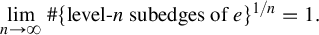 $$ \begin{align*} \lim\limits_{n\rightarrow \infty} \# \{ \text{level-}n \text{ subedges of } e \} ^{1/n} = 1. \end{align*} $$
We say that $\mathcal {R}$
has sub-exponential growth of edge subdivisions if every level-
$\mathcal {R}$
has sub-exponential growth of edge subdivisions if every level- $0$
edge has sub-exponential growth of subdivisions. By Proposition 8.2, we can substitute the term ‘sub-exponential’ for ‘polynomial’.
$0$
edge has sub-exponential growth of subdivisions. By Proposition 8.2, we can substitute the term ‘sub-exponential’ for ‘polynomial’.
Recall that we defined the directed graph of edge subdivisions $\mathcal {E}$
in §4.6. Also recall that a level-
$\mathcal {E}$
in §4.6. Also recall that a level- $0$
edge e is called periodic (or also called recurrent) if the corresponding vertex
$0$
edge e is called periodic (or also called recurrent) if the corresponding vertex $[e]$
in
$[e]$
in $\mathcal {E}$
is contained in a cycle.
$\mathcal {E}$
is contained in a cycle.
Proposition 8.2. A finite subdivision rule $\mathcal {R}$
has sub-exponential growth of edge subdivisions if and only if the cycles in
$\mathcal {R}$
has sub-exponential growth of edge subdivisions if and only if the cycles in $\mathcal {E}$
are disjoint. In this case, for each level-
$\mathcal {E}$
are disjoint. In this case, for each level- $0$
edge e,
$0$
edge e, $\# \{ \text {level-}n \text { subedges of } e \}$
grows polynomially fast as
$\# \{ \text {level-}n \text { subedges of } e \}$
grows polynomially fast as $n\to \infty $
.
$n\to \infty $
.
Let $f^{(1)}:\mathcal {R}^{(1)} \rightarrow \mathcal {R}^{(1)}$
be the restriction of f to the
$f^{(1)}:\mathcal {R}^{(1)} \rightarrow \mathcal {R}^{(1)}$
be the restriction of f to the $1$
-skeleton
$1$
-skeleton $\mathcal {R}^{(1)}$
. Then
$\mathcal {R}^{(1)}$
. Then $f^{(1)}$
is a Markov map. The adjacency matrix of the directed graph of edge subdivision
$f^{(1)}$
is a Markov map. The adjacency matrix of the directed graph of edge subdivision $\mathcal {E}$
coincides with the incidence matrix of the Markov map
$\mathcal {E}$
coincides with the incidence matrix of the Markov map $f^{(1)}$
. The following proposition is immediate from Proposition 3.9.
$f^{(1)}$
. The following proposition is immediate from Proposition 3.9.
Proposition 8.3. A finite subdivision rule $\mathcal {R}$
has polynomial growth of edge subdivisions if and only if
$\mathcal {R}$
has polynomial growth of edge subdivisions if and only if $h_{\textrm {top}}(f^{(1)})=0$
.
$h_{\textrm {top}}(f^{(1)})=0$
.
Let e be a level- $0$
periodic edge. For every
$0$
periodic edge. For every $n>0$
, e has at least one level-n child (subedge) that is recurrent, see §4.7. If e has polynomial growth of subdivisions, then the recurrent subedges are unique at each level. The same statement also works for periodic bands.
$n>0$
, e has at least one level-n child (subedge) that is recurrent, see §4.7. If e has polynomial growth of subdivisions, then the recurrent subedges are unique at each level. The same statement also works for periodic bands.
Proposition 8.4. (Unique recurrent children)
Let $\mathcal {R}$
be a finite subdivision rule and e be a level-
$\mathcal {R}$
be a finite subdivision rule and e be a level- $0$
periodic edge with polynomial growth of subdivisions. For any
$0$
periodic edge with polynomial growth of subdivisions. For any $n \in 1$
, e has a unique level-n subedge that is recurrent. For a level-
$n \in 1$
, e has a unique level-n subedge that is recurrent. For a level- $0$
periodic band
$0$
periodic band $(t;e_1,e_2)$
, if
$(t;e_1,e_2)$
, if $e_1$
and
$e_1$
and $e_2$
have polynomial growth of subdivisions, then for any
$e_2$
have polynomial growth of subdivisions, then for any $n>0$
, there exists a unique level-n subband of
$n>0$
, there exists a unique level-n subband of $(t;e_1,e_2)$
that is recurrent.
$(t;e_1,e_2)$
that is recurrent.
Proof. By Proposition 8.2, there exists a unique cycle in $\mathcal {E}$
passing through
$\mathcal {E}$
passing through $[e]$
. Hence, for any
$[e]$
. Hence, for any $n>0$
, there is only one path of length n from
$n>0$
, there is only one path of length n from $[e]$
and supported within the cycle, which determines a unique level-n recurrent subedge by Proposition 4.5. The uniqueness of a recurrent subedge can also follow from Proposition 8.4.
$[e]$
and supported within the cycle, which determines a unique level-n recurrent subedge by Proposition 4.5. The uniqueness of a recurrent subedge can also follow from Proposition 8.4.
If $(t;e_1,e_2)$
is periodic, then it has at least one level-n unique subband
$(t;e_1,e_2)$
is periodic, then it has at least one level-n unique subband $(t^n;e_1^n,e_2^n)$
. By Lemma 4.9, the level-n edges
$(t^n;e_1^n,e_2^n)$
. By Lemma 4.9, the level-n edges $e^n_1$
and
$e^n_1$
and $e^n_2$
are recurrent subedges of
$e^n_2$
are recurrent subedges of $e_1$
and
$e_1$
and $e_2$
, which are unique by the previous paragraph. Hence, the recurrent subbands are unique at each level.
$e_2$
, which are unique by the previous paragraph. Hence, the recurrent subbands are unique at each level.
Proposition 8.5. Suppose a finite subdivision rule $\mathcal {R}$
has polynomial growth of edge subdivisions. Then every train-track map
$\mathcal {R}$
has polynomial growth of edge subdivisions. Then every train-track map $\phi ^{n+1}_n:N^{n+1} \to N^n$
in the nested sequence of non-expanding spines, defined in Definition 6.18,
$\phi ^{n+1}_n:N^{n+1} \to N^n$
in the nested sequence of non-expanding spines, defined in Definition 6.18,
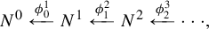 $$ \begin{align*} N^0 \xleftarrow[]{\phi^1_0} N^1 \xleftarrow[]{\phi^2_1} N^2 \xleftarrow[]{\phi^3_2} \cdots\!, \end{align*} $$
is a homeomorphism.
Proof. Let $(t;e_1,e_2)$
be a level-
$(t;e_1,e_2)$
be a level- $0$
periodic band. It follows from Proposition 8.4 and Lemma 4.9 that for any n, there exists a unique level-n recurrent band of
$0$
periodic band. It follows from Proposition 8.4 and Lemma 4.9 that for any n, there exists a unique level-n recurrent band of $(t;e_1,e_2)$
such that its sides are unique level-n recurrent subedges of
$(t;e_1,e_2)$
such that its sides are unique level-n recurrent subedges of $e_1$
and
$e_1$
and $e_2$
. If two level-
$e_2$
. If two level- $0$
periodic bands share a side e, then the level-n recurrent bands also share a side which is the level-n recurrent subedge of e. Hence,
$0$
periodic bands share a side e, then the level-n recurrent bands also share a side which is the level-n recurrent subedge of e. Hence, $N^n$
and
$N^n$
and $N^0$
are made up of the same number of bones of bands which are glued in the same way.
$N^0$
are made up of the same number of bones of bands which are glued in the same way.
Theorem 8.6. Let $\mathcal {R}$
be a finite subdivision rule with polynomial growth of edge subdivisions and f be its subdivision map which is not doubly covered by a torus endomorphism. Let
$\mathcal {R}$
be a finite subdivision rule with polynomial growth of edge subdivisions and f be its subdivision map which is not doubly covered by a torus endomorphism. Let $A\subset \operatorname{Vert}(S_{\mathcal {R}})$
be a set of marked points, that is,
$A\subset \operatorname{Vert}(S_{\mathcal {R}})$
be a set of marked points, that is, $f(A) \cup P_f \subset A$
. Then the following are equivalent.
$f(A) \cup P_f \subset A$
. Then the following are equivalent.
-
(1)
does not have a Levy cycle. -
(2) The level-
$0$
non-expanding spine
$N^0$
does not carry a closed curve that is neither homotopic relative to A to a point nor to some iterate of a peripheral loop of a Julia point in A. -
(3)
is combinatorially equivalent to a unique rational map up to conjugation by Möbius transformations, that is, f does not have a Thurston obstruction.


Proof. $(1) \Leftrightarrow (2)$
follows from Theorem 6.21 and Proposition 8.5. The equivalence with
$(1) \Leftrightarrow (2)$
follows from Theorem 6.21 and Proposition 8.5. The equivalence with $(3)$
follows from Theorem 7.6 and Proposition 8.3.
$(3)$
follows from Theorem 7.6 and Proposition 8.3.
Example 8.7. (Example 6.17 continued)
Removing the edge type C from Figure 9, we have a finite subdivision rule with bounded edge subdivisions. Since the subdivision map is unchanged, there is no Levy cycle by the discussion in Example 6.17. It follows from Theorem 8.6 that there is also no Thurston obstruction.
9 Examples
9.1 Critically fixed rational maps
A rational map is critically fixed if every critical point is a fixed point. It was recently shown that there is a one-to-one correspondence between critically fixed rational functions and planar graphs. The idea started from [Reference Pilgrim and TanPT98] and was completed in [Reference HlushchankaHlu19].
Theorem 9.1. (Hlushchanka, Pilgrim et al)
There is a one-to-one correspondence between the holomorphic conjugacy classes of critically fixed rational functions and the planar isotopy classes of connected planar graphs without loops.
Let G be a planar graph without loops and f be the corresponding critically fixed rational map in Theorem 9.1. At the end of this subsection, we construct a finite rule $\mathcal {R}_G$
such that: (1) its subdivision map is f and (2) every edge never subdivides.
$\mathcal {R}_G$
such that: (1) its subdivision map is f and (2) every edge never subdivides.
Let f be a critically fixed rational map. The Tischler graph of f is a graph embedded in $\hat {\mathbb {C}}$
whose edge set is the collection of fixed internal rays in the immediate attracting basins of all critical points. It follows from [Reference HlushchankaHlu19] that the Tischler graph of any critically fixed rational map is connected.
$\hat {\mathbb {C}}$
whose edge set is the collection of fixed internal rays in the immediate attracting basins of all critical points. It follows from [Reference HlushchankaHlu19] that the Tischler graph of any critically fixed rational map is connected.
To construct a critically fixed rational function from a planar graph without loops, we use the blowing-up an arc construction, which was first introduced in [Reference Pilgrim and TanPT98].
9.1.1 Blowing-up an arc
Let ![]() be a post-critically finite branched covering and
be a post-critically finite branched covering and $\gamma $
be an arc fixed by f. Let
$\gamma $
be an arc fixed by f. Let $D \subset S^2$
be an open
$D \subset S^2$
be an open $2$
-disc contained in a small neighborhood of
$2$
-disc contained in a small neighborhood of $\gamma $
with
$\gamma $
with $\gamma \subset \partial D$
. Let
$\gamma \subset \partial D$
. Let $\gamma '= \partial D - \textrm {int}(\gamma )$
. Define an orientation-preserving continuous map
$\gamma '= \partial D - \textrm {int}(\gamma )$
. Define an orientation-preserving continuous map $g:S^2 \setminus D \rightarrow S^2$
in such a way that g maps
$g:S^2 \setminus D \rightarrow S^2$
in such a way that g maps $\gamma $
and
$\gamma $
and $\gamma '$
to
$\gamma '$
to $\gamma $
, with endpoints fixed. Define another orientation-preserving continuous map
$\gamma $
, with endpoints fixed. Define another orientation-preserving continuous map $h:\overline {D} \rightarrow S^2$
in a similar way so that h maps
$h:\overline {D} \rightarrow S^2$
in a similar way so that h maps $\gamma $
and
$\gamma $
and $\gamma '$
to
$\gamma '$
to $\gamma $
, with endpoints fixed, and maps the D to
$\gamma $
, with endpoints fixed, and maps the D to $S^2 \setminus \gamma $
homeomorphically. A new branched covering
$S^2 \setminus \gamma $
homeomorphically. A new branched covering ![]() is defined by
is defined by $f_\gamma |_{S^2\setminus D}=f \circ g$
and
$f_\gamma |_{S^2\setminus D}=f \circ g$
and $f_\gamma |_{\overline {D}}=f \circ h$
. We call
$f_\gamma |_{\overline {D}}=f \circ h$
. We call $f_\gamma $
the f blown-up along an arc
$f_\gamma $
the f blown-up along an arc $\gamma $
. Note that
$\gamma $
. Note that $\deg (f_\gamma )=\deg (f)+1$
.
$\deg (f_\gamma )=\deg (f)+1$
.
Let G be a planar graph without loops and $A=\operatorname{Vert}(G)$
. Define a post-critically finite branched covering
$A=\operatorname{Vert}(G)$
. Define a post-critically finite branched covering ![]() by blowing up the identity map
by blowing up the identity map ![]() along all edges of G. The combinatorial equivalence class is independent of the order of blowing-up. Each vertex v of G is a critical point of
along all edges of G. The combinatorial equivalence class is independent of the order of blowing-up. Each vertex v of G is a critical point of $f_G$
such that
$f_G$
such that $\deg _v(f_G)=\deg (v)+1$
. If follows from [Reference Pilgrim and TanPT98, Corollary 3] that
$\deg _v(f_G)=\deg (v)+1$
. If follows from [Reference Pilgrim and TanPT98, Corollary 3] that $f_G$
is combinatorially equivalent to a rational map. Because
$f_G$
is combinatorially equivalent to a rational map. Because $f_\gamma $
fixes
$f_\gamma $
fixes $\gamma $
, the branched covering
$\gamma $
, the branched covering $f_G$
is the identity on G. Define a finite subdivision rule
$f_G$
is the identity on G. Define a finite subdivision rule $\mathcal {R}_G$
such that:
$\mathcal {R}_G$
such that:
-
(1)
$S_{\mathcal {R}_G}$
is the CW-complex whose
$1$
-skeleton is G; -
(2)
$\mathcal {R}_G(S_{\mathcal {R}_G})$
is the CW-complex whose
$1$
-skeleton is
$f^{-1}(G)$
; and -
(3)
$f_G:\mathcal {R}_G(S_{\mathcal {R}_G}) \rightarrow S_{\mathcal {R}_G}$
is the subdivision map of
$\mathcal {R}_G$
.


Remark 9.2. When an edge is blown-up, there are two choices for D, depending on which side of $\gamma $
is the disk D. However, the combinatorial equivalence class of the resulting branched covering is independent.
$\gamma $
is the disk D. However, the combinatorial equivalence class of the resulting branched covering is independent.
Example 9.3. See Figure 10. The graph G is a triangle with one more edge attached. Figure 10(a) indicates the disk that we use in blowing-up the edge $\gamma $
. Figures 10(b) and 10(c) indicate the CW-complex structures at level-
$\gamma $
. Figures 10(b) and 10(c) indicate the CW-complex structures at level- $0$
and
$0$
and $1$
. The shaded triangles in Figure 10(c) are mapped to the shaded triangle in Figure 10(b) under the subdivision map
$1$
. The shaded triangles in Figure 10(c) are mapped to the shaded triangle in Figure 10(b) under the subdivision map $f_G$
.
$f_G$
.

Figure 10 Blowing-up arcs of graphs.
9.2 Face-inversion constructions and critically fixed anti-rational maps
The construction in this section was also investigated in [Reference GeyerGey22, Reference Lodge, Luo and MukherjeeLLM22] in the study of critically fixed anti-rational maps.
Let G be a finite graph in the $2$
-sphere
$2$
-sphere $S^2$
. The graph G defines the CW-complex structure
$S^2$
. The graph G defines the CW-complex structure $\mathcal {T}$
with
$\mathcal {T}$
with $\mathcal {T}^{(1)}=G$
. A graph is k-vertex-connected or k-edge-connected if it is not disconnected by the removal of fewer than k vertices or (open) edges, respectively. For the characteristic map
$\mathcal {T}^{(1)}=G$
. A graph is k-vertex-connected or k-edge-connected if it is not disconnected by the removal of fewer than k vertices or (open) edges, respectively. For the characteristic map $\phi _t:\textbf {t} \rightarrow t$
of a closed
$\phi _t:\textbf {t} \rightarrow t$
of a closed $2$
-cell t, we say that the boundary vertices or edges of t are identified if more than one vertex or edge are identified under
$2$
-cell t, we say that the boundary vertices or edges of t are identified if more than one vertex or edge are identified under $\phi _t$
. The following are characterizations of
$\phi _t$
. The following are characterizations of $2$
- or
$2$
- or $3$
-connectivity of graphs embedded in
$3$
-connectivity of graphs embedded in $S^2$
.
$S^2$
.
-
• G is
$2$
-vertex-connected if and only if boundary vertices of every
$2$
-cell are not identified, that is, the boundary of every
$2$
-cell is a Jordan curve. -
• G is
$2$
-edge-connected if and only if the boundary edges of every
$2$
-cell are not identified. The
$2$
-vertex connectedness implies the
$2$
-edge connectedness. -
• G is
$3$
-edge-connected if and only if it is
$2$
-edge-connected and any two
$2$
-cells do not share more than one edge. It is also equivalent to the dual graph having no cycle of length
$\le 2$
.


Assume G is $2$
-vertex-connected and
$2$
-vertex-connected and $\deg (v)\ge 3$
for every
$\deg (v)\ge 3$
for every $v\in \operatorname{Vert}(G)$
. Let t be a
$v\in \operatorname{Vert}(G)$
. Let t be a $2$
-cell of
$2$
-cell of $\mathcal {T}$
and
$\mathcal {T}$
and $\sigma _t$
be the reflection of
$\sigma _t$
be the reflection of $S^2$
in
$S^2$
in $\partial t$
. This is possible because the
$\partial t$
. This is possible because the $2$
-vertex-connectedness implies that
$2$
-vertex-connectedness implies that $\partial t$
is a simple closed curve. Then
$\partial t$
is a simple closed curve. Then $\sigma _t(G)$
is a graph isomorphic to G such that
$\sigma _t(G)$
is a graph isomorphic to G such that $\sigma _t(G)\cap G = \partial t$
. Define a graph H by
$\sigma _t(G)\cap G = \partial t$
. Define a graph H by
 $$ \begin{align*} H=\bigcup\limits_{t \text{ is a 2-cell of } \mathcal{T}} \sigma_t(G). \end{align*} $$
Let $\mathcal {T}'$
be the CW-complex structure on
$\mathcal {T}'$
be the CW-complex structure on $S^2$
with
$S^2$
with $\mathcal {T}^{\prime (1)}=H$
. We define a finite subdivision rule as follows: let
$\mathcal {T}^{\prime (1)}=H$
. We define a finite subdivision rule as follows: let $S_{\mathcal {R}}=\mathcal {T}$
and
$S_{\mathcal {R}}=\mathcal {T}$
and $\mathcal {R}(S_{\mathcal {R}})=\mathcal {T}'$
. Define an orientation reversing branched self-covering
$\mathcal {R}(S_{\mathcal {R}})=\mathcal {T}'$
. Define an orientation reversing branched self-covering ![]() defined by
defined by $f|_t=\sigma _t|_t$
for every
$f|_t=\sigma _t|_t$
for every $2$
-cell t of
$2$
-cell t of $S_{\mathcal {R}}$
. Then f becomes a subdivision map
$S_{\mathcal {R}}$
. Then f becomes a subdivision map $f:\mathcal {R}(S_{\mathcal {R}}) \rightarrow S_{\mathcal {R}}$
. Note that every edge does not subdivide. The degree of f is equal to the number of
$f:\mathcal {R}(S_{\mathcal {R}}) \rightarrow S_{\mathcal {R}}$
. Note that every edge does not subdivide. The degree of f is equal to the number of $2$
-cells of
$2$
-cells of $\mathcal {T}$
minus one. We call
$\mathcal {T}$
minus one. We call $\mathcal {R}$
the finite subdivision rule of face-inversion of G. Every vertex
$\mathcal {R}$
the finite subdivision rule of face-inversion of G. Every vertex $v\in \operatorname{Vert}(G)$
is a fixed critical point of
$v\in \operatorname{Vert}(G)$
is a fixed critical point of $\deg _v(f)=\deg (v)-1$
.
$\deg _v(f)=\deg (v)-1$
.
A natural way to obtain an orientation preserving finite subdivision rule is to take the square of the subdivision $\mathcal {R}^2$
and the subdivision map
$\mathcal {R}^2$
and the subdivision map $f^2:\mathcal {R}^2(\mathcal {T})\rightarrow \mathcal {T}$
. We denote by
$f^2:\mathcal {R}^2(\mathcal {T})\rightarrow \mathcal {T}$
. We denote by $\mathcal {R}_{sq}$
this squared orientation preserving subdivision rule. Another way is to post-compose with an orientation-reversing automorphism of G. An automorphism
$\mathcal {R}_{sq}$
this squared orientation preserving subdivision rule. Another way is to post-compose with an orientation-reversing automorphism of G. An automorphism $\tau \in \operatorname {\textrm {Aut}}(G)$
is called orientation reversing if it extends to an orientation-reversing homeomorphism of
$\tau \in \operatorname {\textrm {Aut}}(G)$
is called orientation reversing if it extends to an orientation-reversing homeomorphism of $S^2$
. For any orientation-reversing automorphism
$S^2$
. For any orientation-reversing automorphism $\tau \in \operatorname {\textrm {Aut}}(G)$
, we have an orientation preserving subdivision map
$\tau \in \operatorname {\textrm {Aut}}(G)$
, we have an orientation preserving subdivision map $f_\tau :=\tau \circ f:\mathcal {R}(S_{\mathcal {R}}) \rightarrow S_{\mathcal {R}}$
defined on the same subdivision complexes as
$f_\tau :=\tau \circ f:\mathcal {R}(S_{\mathcal {R}}) \rightarrow S_{\mathcal {R}}$
defined on the same subdivision complexes as $\mathcal {R}$
. Denote this finite subdivision rule by
$\mathcal {R}$
. Denote this finite subdivision rule by $\mathcal {R}_\tau $
.
$\mathcal {R}_\tau $
.
Theorem 9.4. Let G be a $2$
-vertex-connected graph in
$2$
-vertex-connected graph in $S^2$
such that
$S^2$
such that $\deg (v)\ge 3$
for every
$\deg (v)\ge 3$
for every $v\in \operatorname{Vert}(G)$
. Let
$v\in \operatorname{Vert}(G)$
. Let $\mathcal {R}$
be the finite subdivision rule of the face-inversion of G and
$\mathcal {R}$
be the finite subdivision rule of the face-inversion of G and $f:\mathcal {R}(S_{\mathcal {R}})\rightarrow S_{\mathcal {R}}$
be its subdivision map. Let
$f:\mathcal {R}(S_{\mathcal {R}})\rightarrow S_{\mathcal {R}}$
be its subdivision map. Let $\tau $
be any orientation-reversing automorphism of G. Then the following are equivalent:
$\tau $
be any orientation-reversing automorphism of G. Then the following are equivalent:
-
(1) G is
$3$
-edge-connected; -
(2)
does not have a Levy cycle; -
(2’)
does not have a Thurston obstruction; -
(3)
does not have a Levy cycle; -
(3’)
does not have a Thurston obstruction.

Proof. A level- $0$
band
$0$
band $b=(t;e_1,e_2)$
is non-separating if and only if there is another level-
$b=(t;e_1,e_2)$
is non-separating if and only if there is another level- $0$
band
$0$
band $b'=(t';e^{\prime }_1,e^{\prime }_2)$
such that
$b'=(t';e^{\prime }_1,e^{\prime }_2)$
such that $e_1=e_1^{\prime }$
,
$e_1=e_1^{\prime }$
, $e_2=e_2^{\prime }$
, and
$e_2=e_2^{\prime }$
, and $t\neq t'$
. If such bands b and
$t\neq t'$
. If such bands b and $b'$
exist, the removal of two edges of G intersecting the bones of these bands disconnects G, that is, G is not
$b'$
exist, the removal of two edges of G intersecting the bones of these bands disconnects G, that is, G is not $3$
-edge-connected. Conversely, if G is not
$3$
-edge-connected. Conversely, if G is not $3$
-edge-connected, then such level-
$3$
-edge-connected, then such level- $0$
bands b and
$0$
bands b and $b'$
exist. Hence, G is
$b'$
exist. Hence, G is $3$
-edge-connected if and only if every level-
$3$
-edge-connected if and only if every level- $0$
band is non-separating. In the case, the level-
$0$
band is non-separating. In the case, the level- $0$
non-expanding spine for
$0$
non-expanding spine for $\mathcal {R}_{sq}$
is an empty set. Then
$\mathcal {R}_{sq}$
is an empty set. Then $(1)\Rightarrow (2)\Leftrightarrow (2')$
follows from Theorem 8.6.
$(1)\Rightarrow (2)\Leftrightarrow (2')$
follows from Theorem 8.6.
Assume G is not $3$
-edge-connected so that there are bands b and
$3$
-edge-connected so that there are bands b and $b'$
described as in the previous paragraph. The union of bones of b and
$b'$
described as in the previous paragraph. The union of bones of b and $b'$
is a homotopically infinite circle contained in the level-
$b'$
is a homotopically infinite circle contained in the level- $0$
non-expanding spine
$0$
non-expanding spine $N^0$
of
$N^0$
of $\mathcal {R}_{sq}$
. Hence,
$\mathcal {R}_{sq}$
. Hence, $(2) \Rightarrow (1)$
follows from Theorem 8.6.
$(2) \Rightarrow (1)$
follows from Theorem 8.6.
The equivalence $(2) \Leftrightarrow (3)$
follows from the fact that the subdivisions
$(2) \Leftrightarrow (3)$
follows from the fact that the subdivisions $\mathcal {R}^n(S_{\mathcal {R}})$
and
$\mathcal {R}^n(S_{\mathcal {R}})$
and $\mathcal {R}_\tau ^n(S_{\mathcal {R}_\tau })$
have the same CW-complex structure. The level-
$\mathcal {R}_\tau ^n(S_{\mathcal {R}_\tau })$
have the same CW-complex structure. The level- $2n$
non-expanding spine of
$2n$
non-expanding spine of $\mathcal {R}_\tau $
is equal to the level-n non-expanding spine of
$\mathcal {R}_\tau $
is equal to the level-n non-expanding spine of $\mathcal {R}_{sq}$
for
$\mathcal {R}_{sq}$
for $n\ge 0$
.
$n\ge 0$
.
Remark 9.5. The equivalence $(1)\Leftrightarrow (2) \Leftrightarrow (2')$
is also shown in [Reference GeyerGey22, Theorem 5.8] and [Reference Lodge, Luo and MukherjeeLLM22, Proposition 4.10].
$(1)\Leftrightarrow (2) \Leftrightarrow (2')$
is also shown in [Reference GeyerGey22, Theorem 5.8] and [Reference Lodge, Luo and MukherjeeLLM22, Proposition 4.10].
Remark 9.6. For an orientation reversing branched covering f, $f^2$
is combinatorially equivalent to a rational map if and only if f is combinatorially equivalent to a anti-rational map. See [Reference GeyerGey22, Theorem 3.9] and [Reference Lodge, Lyubich, Merenkov and MukherjeeLLMM23, Proposition 6.1].
$f^2$
is combinatorially equivalent to a rational map if and only if f is combinatorially equivalent to a anti-rational map. See [Reference GeyerGey22, Theorem 3.9] and [Reference Lodge, Lyubich, Merenkov and MukherjeeLLMM23, Proposition 6.1].
Remark 9.7. Even if there exists a vertex v with $\deg (v)=2$
, the construction is still well defined, but v is not a critical point. Note that such a vertex v can be removed from the vertex set without any change in the face-inversion construction.
$\deg (v)=2$
, the construction is still well defined, but v is not a critical point. Note that such a vertex v can be removed from the vertex set without any change in the face-inversion construction.
Example 9.8. See Figure 11. Let G be the graph on the bottom and $\tau $
the reflection along the middle horizontal line. Then the left and right subdivisions represent
$\tau $
the reflection along the middle horizontal line. Then the left and right subdivisions represent $\mathcal {R}_\tau $
and
$\mathcal {R}_\tau $
and $\mathcal {R}$
, respectively.
$\mathcal {R}$
, respectively.
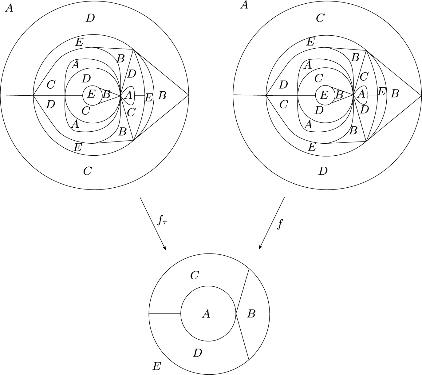
Figure 11 Finite subdivision rules defined from the face-inversion of a planar graph.
To obtain an explicit formula of $f_\tau (z)={p(z)}/{q(z)}$
, we normalize three vertices on the axis of
$f_\tau (z)={p(z)}/{q(z)}$
, we normalize three vertices on the axis of $\tau $
in Figure 11 from left to right to
$\tau $
in Figure 11 from left to right to $0,1$
, and
$0,1$
, and $\infty $
. Note that
$\infty $
. Note that $\deg _z(f_\tau )$
is
$\deg _z(f_\tau )$
is $2$
at
$2$
at $z=0$
or
$z=0$
or $1$
, and
$1$
, and $\deg _z(f_\tau )$
is
$\deg _z(f_\tau )$
is $3$
at
$3$
at $z=\infty $
. Since
$z=\infty $
. Since $0$
and
$0$
and $\infty $
are fixed points,
$\infty $
are fixed points, $p(z)$
is a quartic polynomial divided by
$p(z)$
is a quartic polynomial divided by $z^2$
, and
$z^2$
, and $q(z)$
is a linear polynomial. We may assume that
$q(z)$
is a linear polynomial. We may assume that $q(z)$
is monic. The conditions are that: (1)
$q(z)$
is monic. The conditions are that: (1) $z=1$
is a critical fixed point and (2) the other two critical points are exchanged by
$z=1$
is a critical fixed point and (2) the other two critical points are exchanged by $f(z)$
give rise to a system of equation about coefficients of
$f(z)$
give rise to a system of equation about coefficients of $p(z)$
and
$p(z)$
and $q(z)$
. Solving this numerically, we have
$q(z)$
. Solving this numerically, we have
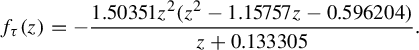 $$ \begin{align*} f_\tau(z)=-\frac{1.50351z^2(z^2-1.15757z-0.596204)}{z+0.133305}. \end{align*} $$
See Figure 12 for the Julia set.
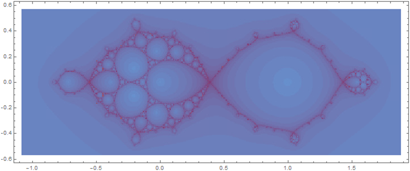
Figure 12 Julia set of $z\mapsto -{1.50351z^2(z^2-1.15757z-0.596204)}/{z+0.133305}$
.
$z\mapsto -{1.50351z^2(z^2-1.15757z-0.596204)}/{z+0.133305}$
.
9.3 Finite subdivision rules with essential non-expanding spines at higher levels
In this subsection, we prove Proposition 9.9 by constructing an example.
Proposition 9.9. For every $N>0$
, there exists a finite subdivision rule
$N>0$
, there exists a finite subdivision rule $\mathcal {R}_N$
with the subdivision map
$\mathcal {R}_N$
with the subdivision map $f_{\mathcal {R}_N}:\mathcal {R}_N(S_{\mathcal {R}_N}) \to S_{\mathcal {R}_N}$
of degree
$f_{\mathcal {R}_N}:\mathcal {R}_N(S_{\mathcal {R}_N}) \to S_{\mathcal {R}_N}$
of degree $6$
such that: (1)
$6$
such that: (1) $\operatorname{Vert}(S_{\mathcal {R}_N})=P_{f_{\mathcal {R}_N}}$
; (2) the level-k non-expanding spine
$\operatorname{Vert}(S_{\mathcal {R}_N})=P_{f_{\mathcal {R}_N}}$
; (2) the level-k non-expanding spine $N^k$
is essential relative to
$N^k$
is essential relative to $\operatorname{Vert}(S_{\mathcal {R}_N})$
for
$\operatorname{Vert}(S_{\mathcal {R}_N})$
for $k<N$
; and (3)
$k<N$
; and (3) $N^k$
is not essential relative to
$N^k$
is not essential relative to $\operatorname{Vert}(S_{\mathcal {R}_N})$
for
$\operatorname{Vert}(S_{\mathcal {R}_N})$
for $k\ge N$
.
$k\ge N$
.
Let us see the finite subdivision rule $\mathcal {R}$
in Figure 13. The
$\mathcal {R}$
in Figure 13. The $1$
-skeleton at level-
$1$
-skeleton at level- $0$
is drawn by bold curves. The non-expanding spines
$0$
is drawn by bold curves. The non-expanding spines $N^0$
and
$N^0$
and $N^1$
are drawn by dotted curves. The
$N^1$
are drawn by dotted curves. The $N^0$
is essential but
$N^0$
is essential but $N^1$
is homotopically trivial. Let f be the subdivision map described in Figure 13. We modify the finite subdivision rule
$N^1$
is homotopically trivial. Let f be the subdivision map described in Figure 13. We modify the finite subdivision rule $\mathcal {R}$
into
$\mathcal {R}$
into $\mathcal {R}'$
as follows.
$\mathcal {R}'$
as follows.
-
(1) Change the labels A and B into
$A_1$
and
$B_1$
. -
(2) For
$2 \le i\le n$
, we draw
$n-1$
copies of annuli consisting of
$A_i$
and
$B_i$
in a row on the left of the annulus consisting of
$A_1$
and
$B_1$
at level-
$0$
. Denote by
$S_{\mathcal {R}'}$
the modified level-
$0$
CW-complex. Define
$\mathcal {R}'(S_{\mathcal {R}'})=f^{-1}(S_{\mathcal {R}'})$
. -
(3) Let
$\sigma $
be an orientation-preserving homeomorphism of the
$2$
-sphere such that
$\sigma (S_{\mathcal {R}'})=S_{\mathcal {R}'}$
, and
$\sigma (A_i)=A_{i+1}$
and
$\sigma (B_i)=B_{i+1}$
for any
$1 \le i\le n$
, where indices are considered modulo n. That is,
$\sigma $
is a
$1/n$
-rotation. Define the subdivision map
$f':\mathcal {R}'(S_{\mathcal {R}'})\to S_{\mathcal {R}'}$
by
$f'=\sigma \circ f$
.


Figure 13 A degree $6$
finite subdivision rule with six tile types.
$6$
finite subdivision rule with six tile types.
Let $N^{\prime i}$
be the level-i non-expanding spine of
$N^{\prime i}$
be the level-i non-expanding spine of $\mathcal {R}'$
. The
$\mathcal {R}'$
. The $N^{\prime 0}$
is n-copies of circles. The
$N^{\prime 0}$
is n-copies of circles. The $N^{\prime 1}$
is the union of
$N^{\prime 1}$
is the union of $n-1$
-copies of circles with three non-closed curves. Similarly, for
$n-1$
-copies of circles with three non-closed curves. Similarly, for $k<n$
, the level-k non-expanding spine
$k<n$
, the level-k non-expanding spine $N^{\prime k}$
has
$N^{\prime k}$
has $n-k$
circles and some non-closed curves. Therefore,
$n-k$
circles and some non-closed curves. Therefore, $N^{\prime i}$
is essential if
$N^{\prime i}$
is essential if $i<n$
and non-essential if
$i<n$
and non-essential if $i\ge n$
.
$i\ge n$
.
9.4 Edge–edge expansion versus edge subdivisions
Let us further investigate the equivalence between the existence of Levy cycles and of Thurston obstructions. Recall that the coefficients of Thurston linear transformation are defined by
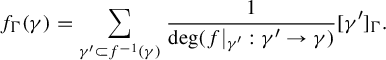 $$ \begin{align*} f_\Gamma (\gamma)=\sum\limits_{\gamma'\subset f^{-1}(\gamma)}\frac{1}{\deg (f|_{\gamma'}:\gamma' \to \gamma)} [\gamma']_\Gamma. \end{align*} $$
In the setting of finite subdivision rules, the summands ${1}/{\deg }$
are related to the expansion between edges and the number of summands is related to the growth rate of edge subdivisions. Hence, we can expect there is no Thurston obstruction if the edge–edge expansion dominates the edge subdivisions. See [Reference Cui, Peng and TanCPT16, Theorem 8.4] for a similar comparison.
${1}/{\deg }$
are related to the expansion between edges and the number of summands is related to the growth rate of edge subdivisions. Hence, we can expect there is no Thurston obstruction if the edge–edge expansion dominates the edge subdivisions. See [Reference Cui, Peng and TanCPT16, Theorem 8.4] for a similar comparison.
Let $\mathcal {R}$
be a finite subdivision rule.
$\mathcal {R}$
be a finite subdivision rule.
Edge–edge expansion. We say that $\mathcal {R}$
is edge–edge
$\mathcal {R}$
is edge–edge $\unicode{x3bb} $
-expanding for
$\unicode{x3bb} $
-expanding for $\unicode{x3bb} \ge 1$
if there exists
$\unicode{x3bb} \ge 1$
if there exists $C>0$
such that for any
$C>0$
such that for any $n\ge 0$
and any bone
$n\ge 0$
and any bone $\gamma $
of level-
$\gamma $
of level- $0$
band, the level-n subdivision complex
$0$
band, the level-n subdivision complex $\mathcal {R}^n(S_{\mathcal {R}})$
subdivides
$\mathcal {R}^n(S_{\mathcal {R}})$
subdivides $\gamma $
into at least
$\gamma $
into at least $C\cdot \unicode{x3bb} ^n$
segments.
$C\cdot \unicode{x3bb} ^n$
segments.
Edge subdivision rate. For any level- $0$
edge e, the exponential growth rate of subdivisions of e is the number
$0$
edge e, the exponential growth rate of subdivisions of e is the number $\nu _e\ge 1$
with
$\nu _e\ge 1$
with $\lim _{n\to \infty }(\#\{\textrm {level}\mbox {-}\textrm {n subedges of } e\})^{1/n}= \nu _e$
. The maximum
$\lim _{n\to \infty }(\#\{\textrm {level}\mbox {-}\textrm {n subedges of } e\})^{1/n}= \nu _e$
. The maximum $\nu :=\max ~\nu _e$
over level-
$\nu :=\max ~\nu _e$
over level- $0$
edges e is called the maximal exponential growth rate of edge subdivisions.
$0$
edges e is called the maximal exponential growth rate of edge subdivisions.
Proposition 9.10. Let $\mathcal {R}$
be a finite subdivision rule. Let
$\mathcal {R}$
be a finite subdivision rule. Let $\nu $
be the maximal exponential growth rate of edge subdivisions. If
$\nu $
be the maximal exponential growth rate of edge subdivisions. If $\mathcal {R}$
is edge–edge
$\mathcal {R}$
is edge–edge $\unicode{x3bb} $
-expanding for some
$\unicode{x3bb} $
-expanding for some $\unicode{x3bb}>1$
, then the non-expanding spine of
$\unicode{x3bb}>1$
, then the non-expanding spine of $\mathcal {R}$
is empty so that the subdivision map
$\mathcal {R}$
is empty so that the subdivision map ![]() does not have a Levy cycle for any set of marked points A. Moreover, if
does not have a Levy cycle for any set of marked points A. Moreover, if $\unicode{x3bb}>\nu $
, then the subdivision map
$\unicode{x3bb}>\nu $
, then the subdivision map ![]() does not have a Thurston obstruction for any set of marked points A.
does not have a Thurston obstruction for any set of marked points A.
Proof. The first part about the emptiness of non-expanding spines immediately follows from the definition of a non-expanding spine. Let us assume $\unicode{x3bb}>\nu $
and show the second part. Let
$\unicode{x3bb}>\nu $
and show the second part. Let $\Gamma =\{\gamma _1,\gamma _2,\ldots ,\gamma _k\}$
be a multicurve of
$\Gamma =\{\gamma _1,\gamma _2,\ldots ,\gamma _k\}$
be a multicurve of $(S^2,A)$
. For a closed curve
$(S^2,A)$
. For a closed curve $\gamma $
transverse to
$\gamma $
transverse to $\mathcal {R}^n(S_{\mathcal {R}})$
, we denote by
$\mathcal {R}^n(S_{\mathcal {R}})$
, we denote by $l_n(\gamma )$
the cardinality of the intersection
$l_n(\gamma )$
the cardinality of the intersection $(\mathcal {R}^n(S_{\mathcal {R}}))^{(1)} \cap \gamma $
. Let
$(\mathcal {R}^n(S_{\mathcal {R}}))^{(1)} \cap \gamma $
. Let $C_0:=\min _{i\neq j} {l_0(\gamma _i)}/{l_0(\gamma _j)}$
. Since
$C_0:=\min _{i\neq j} {l_0(\gamma _i)}/{l_0(\gamma _j)}$
. Since $\mathcal {R}$
is edge–edge
$\mathcal {R}$
is edge–edge $\unicode{x3bb} $
-expanding, there exists
$\unicode{x3bb} $
-expanding, there exists $C_1>0$
such that for any
$C_1>0$
such that for any $\gamma _i\in \Gamma $
and for any connected component
$\gamma _i\in \Gamma $
and for any connected component $\gamma _i^{\prime }$
of
$\gamma _i^{\prime }$
of $f^{-n}(\gamma _i)$
, we have
$f^{-n}(\gamma _i)$
, we have
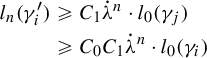 $$ \begin{align*} l_n(\gamma^{\prime}_i) &\ge C_1\dot{\unicode{x3bb}}^n \cdot l_0(\gamma_j)\\ &\ge C_0 C_1 \dot{\unicode{x3bb}}^n \cdot l_0(\gamma_i) \end{align*} $$
for any $n\ge 0$
, where
$n\ge 0$
, where $\gamma _j\in \Gamma $
is isotopic to
$\gamma _j\in \Gamma $
is isotopic to $\gamma ^{\prime }_i$
. Then
$\gamma ^{\prime }_i$
. Then $\deg (f:\gamma _i^{\prime }\to \gamma _i)\ge C_0C_1\unicode{x3bb} ^n$
.
$\deg (f:\gamma _i^{\prime }\to \gamma _i)\ge C_0C_1\unicode{x3bb} ^n$
.
Let $C_2$
be the minimal number satisfying
$C_2$
be the minimal number satisfying $|e\cap \Gamma |\le C_2$
for any level-
$|e\cap \Gamma |\le C_2$
for any level- $0$
edge e. It follows that (a) for any level-n edge
$0$
edge e. It follows that (a) for any level-n edge $e^n$
,
$e^n$
, $|e^n \cap f^{-n}(\Gamma )| \le C_2$
. By the definition of
$|e^n \cap f^{-n}(\Gamma )| \le C_2$
. By the definition of $\nu $
, there exists
$\nu $
, there exists $C_3>0$
such that for any level-
$C_3>0$
such that for any level- $0$
edge e and any
$0$
edge e and any $n\ge 0$
, the number of level-n subedges of e is at most
$n\ge 0$
, the number of level-n subedges of e is at most $C_3 \cdot {\nu '}^n$
for some
$C_3 \cdot {\nu '}^n$
for some ${\nu '}$
with
${\nu '}$
with $\unicode{x3bb}> \nu '>\nu $
. Consider a concatenation
$\unicode{x3bb}> \nu '>\nu $
. Consider a concatenation $\alpha $
of level-
$\alpha $
of level- $0$
edges connecting two points
$0$
edges connecting two points $a_1,a_2\in A$
with
$a_1,a_2\in A$
with $a_1$
and
$a_1$
and $a_2$
being in the different Jordan domains of
$a_2$
being in the different Jordan domains of $\gamma _i$
. Note that (b) every simple closed curve isotopic to
$\gamma _i$
. Note that (b) every simple closed curve isotopic to $\gamma _i$
has at least one intersection point with
$\gamma _i$
has at least one intersection point with $\alpha $
. We have
$\alpha $
. We have
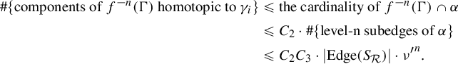 $$ \begin{align*} \# \{\textrm{components of } f^{-n}(\Gamma) \textrm{ homotopic to } \gamma_i\} &\le \textrm{the cardinality of } f^{-n}(\Gamma) \cap \alpha\\ &\le C_2 \cdot \#\{\textrm{level}\mbox{-}\textrm{n subedges of } \alpha\}\\ &\le C_2 C_3\cdot|\!\operatorname{\textrm{Edge}}(S_{\mathcal{R}})|\cdot {\nu'}^n. \end{align*} $$
The first inequality follows from item (b), the second follows from item (a) and the third follows from the fact that $\alpha $
is a concatenation of at most
$\alpha $
is a concatenation of at most $|\!\operatorname {\textrm {Edge}}(S_{\mathcal {R}})|$
edges at level-
$|\!\operatorname {\textrm {Edge}}(S_{\mathcal {R}})|$
edges at level- $0$
.
$0$
.
Hence, every entry in the Thurston linear transformation is bounded from above by
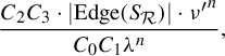 $$ \begin{align*} \frac{C_2 C_3\cdot|\!\operatorname{\textrm{Edge}}(S_{\mathcal{R}})|\cdot {\nu'} ^n}{C_0C_1\unicode{x3bb}^n}, \end{align*} $$
which tends to 0 as $n \to \infty $
. Then the map f does not allow any Thurston obstruction.
$n \to \infty $
. Then the map f does not allow any Thurston obstruction.
There are many ways to improve Proposition 9.10. Here are two possible directions.
Suggestion 1. Proposition 9.10 can be compared with [Reference Floyd, Parry and PilgrimFPP18b, Proposition 5.1], which states that if $\mathcal {R}$
is edge separating and vertex separating, then the subdivision map does not have a Levy cycle. One difference is that the subdivision map in Proposition 9.10 has to be of hyperbolic type, that is, every critical point is a Fatou point, but [Reference Floyd, Parry and PilgrimFPP18b, Proposition 5.1] works for any subdivision map. The definition of edge separation in [Reference Floyd, Parry and PilgrimFPP18b] is the edge–edge expansion, defined in this article, only for pairs of edges that do not share end points. The vertex separation might be necessary only for Julia vertices. One might be able to obtain a stronger result by combining these two propositions.
$\mathcal {R}$
is edge separating and vertex separating, then the subdivision map does not have a Levy cycle. One difference is that the subdivision map in Proposition 9.10 has to be of hyperbolic type, that is, every critical point is a Fatou point, but [Reference Floyd, Parry and PilgrimFPP18b, Proposition 5.1] works for any subdivision map. The definition of edge separation in [Reference Floyd, Parry and PilgrimFPP18b] is the edge–edge expansion, defined in this article, only for pairs of edges that do not share end points. The vertex separation might be necessary only for Julia vertices. One might be able to obtain a stronger result by combining these two propositions.
Suggestion 2. It would be possible to combine Theorem 7.6 and Proposition 9.10 to obtain a stronger sufficient condition for the equivalence between the existence of Levy and Thurston obstructions. We might be able to: (1) have the equivalence on the part where edges subdivide polynomially fast and (2) exclude Thurston obstructions where edges subdivide exponentially fast by assuming the condition in Proposition 9.10.
Example 9.11. See Figure 14. We think of the doubles of the left triangle and get the level- $0$
subdivision complex
$0$
subdivision complex $S_{\mathcal {R}}$
with two tiles. Similarly, take the double of the right large triangle, which is subdivided into 12 small triangles, and define it as the level-
$S_{\mathcal {R}}$
with two tiles. Similarly, take the double of the right large triangle, which is subdivided into 12 small triangles, and define it as the level- $1$
complex
$1$
complex $\mathcal {R}(S_{\mathcal {R}})$
. Then Figure 14 defines a finite subdivision rule
$\mathcal {R}(S_{\mathcal {R}})$
. Then Figure 14 defines a finite subdivision rule $\mathcal {R}$
with the subdivision map
$\mathcal {R}$
with the subdivision map $f:\mathcal {R}(S_{\mathcal {R}})\to S_{\mathcal {R}}$
which is defined by a map sending each small triangle on the right to a triangle on the left or its copy with the types of edges being preserved. Then
$f:\mathcal {R}(S_{\mathcal {R}})\to S_{\mathcal {R}}$
which is defined by a map sending each small triangle on the right to a triangle on the left or its copy with the types of edges being preserved. Then $\deg (f)=12$
and f has three critical values
$\deg (f)=12$
and f has three critical values $u,v$
, and w, which are vertices of the level-
$u,v$
, and w, which are vertices of the level- $0$
triangles. Moreover,
$0$
triangles. Moreover, $f(u)=f(v)=f(w)=w$
.
$f(u)=f(v)=f(w)=w$
.
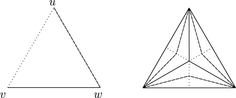
Figure 14 A finite subdivision rule with $\unicode{x3bb}>\nu $
.
$\unicode{x3bb}>\nu $
.
It is immediate that the non-expanding spine is an empty set. By Theorem 6.21, f does not have a Levy cycle. Since $\mathcal {R}$
has exponential growth rate of edge subdivisions, we cannot apply Theorem 8.6 to claim that f does not have a Thurston obstruction. However, it is easy to show that
$\mathcal {R}$
has exponential growth rate of edge subdivisions, we cannot apply Theorem 8.6 to claim that f does not have a Thurston obstruction. However, it is easy to show that $\unicode{x3bb} =4$
and
$\unicode{x3bb} =4$
and $\nu =2$
, and then f does not have a Thurston obstruction by Proposition 9.10.
$\nu =2$
, and then f does not have a Thurston obstruction by Proposition 9.10.
Acknowledgements
The author thanks Dylan Thurston and Kevin Pilgrim for helpful comments and discussions. Without their support and suggestions, this work would not have existed. The author also thanks Dzmitry Dudko for critical comments on the previous version of this article. The author thanks the reviewer for helpful comments and suggestions, which inspired the author to write §9.4. The author also thanks the developers of Xaos and Mathematica, which were used to draw Julia sets in the present article.


 Open access